| Enduring Understanding | Learning Objective | Essential Knowledge |
|---|---|---|
VAR-1 | VAR-1.A |
|
Exploring One-Variable Data
AP Statistics · Topic 1
 9:03
Exploring One-Variable Data
Measure the same thing twenty times and you will not get the same answer twenty times. Twenty students measure the same table. The values vary. That is not a…
English narration · English + 中文 subtitles burned in
1.1
Introducing Statistics: What Can We Learn from Data?

Syllabus
Source: College Board AP Course and Exam Description
Two companies both offer you a first job at $\$36{,}000$ a year. One has a higher median salary; the other has a few very high salaries and a wider spread. Which offer is better for you? A single number cannot say. To answer, you need the whole distribution, described with the right summaries and in context. That is what this unit teaches.
Statistics 统计学 is the science of learning from data 数据 – numbers or labels collected from the real world. Data vary, so we describe patterns and account for the variation 变异 rather than expecting every value to match. A statistical question anticipates an answer based on data that vary. A number on its own means little: "$42$" is meaningless, but "$42\%$ of students in the sample walk to school" carries information because it has context.
Two distinctions run through the whole course. A parameter 参数 is a numerical summary of a whole population; a statistic 统计量 is a numerical summary of a sample - we use the statistic to estimate the parameter we cannot measure directly. And descriptive statistics 描述统计学 only summarise the data set in hand, while inferential statistics 推断统计 use a sample to make and test claims about the larger population.
Explore
Data that varies
Real data spread out across values — statistics finds the pattern in that variation.
Vocabulary
Train
| English |
|---|
| Statistics/stəˈtɪstɪks/ |
| data/ˈdeɪtə/ |
| variation/ˌveərɪˈeɪʃn/ |
| parameter/pəˈræmɪtə/ |
| statistic/stəˈtɪstɪk/ |
| descriptive statistics/dɪˈskrɪptɪv stəˈtɪstɪks/ |
| inferential statistics/ɪnfəˈrenʃl stəˈtɪstɪks/ |
1.2
The Language of Variation: Variables

Syllabus
| Enduring Understanding | Learning Objective | Essential Knowledge |
|---|---|---|
VAR-1 | VAR-1.B |
|
VAR-1.C |
|
Source: College Board AP Course and Exam Description
A variable 变量 is a characteristic that can differ between individuals. Two kinds:
- Categorical 分类 (qualitative): values are labels/groups (eye colour, brand).
- Quantitative 定量: values are numbers you can do arithmetic on (height, age). Quantitative variables are discrete (countable) or continuous (measured).
Choosing the right graph and summary depends on which kind you have.
Explore
Categorical or quantitative?
Every variable is either categorical (it labels each unit with a group) or quantitative (a measured number you can average). Which kind it is decides the graphs and summaries you are allowed to use.
Vocabulary
Train
| English |
|---|
| variable/ˈveərɪəbl/ |
| Categorical/ˌkætɪˈɡɒrɪkl/ |
| Quantitative/ˈkwɒntɪteɪtɪv/ |
1.3
Representing a Categorical Variable with Tables
Syllabus
| Enduring Understanding | Learning Objective | Essential Knowledge |
|---|---|---|
UNC-1 | UNC-1.A |
|
UNC-1.B |
|
Source: College Board AP Course and Exam Description
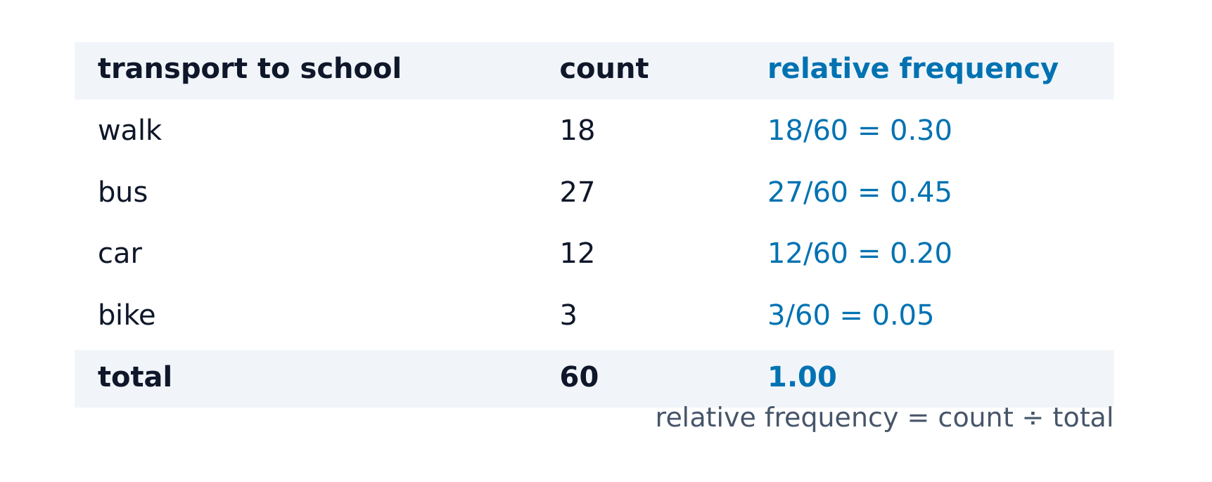
A frequency table 频数表 lists each category's count (frequency); a relative frequency 相对频率 table lists each category's proportion 比例 (count ÷ total). Relative frequencies let you compare groups of different sizes fairly. A proportion, a percentage and a rate all say the same thing: $30$ out of $200$ is $0.15$, $15\%$, or a rate of $150$ per $1000$.
Worked example. In a survey, $36$ of $120$ juniors and $45$ of $200$ seniors said they drive to school. More seniors drive ($45>36$), but that is only because more seniors were asked. Compare proportions: $36/120=0.30$ for juniors and $45/200=0.225$ for seniors. A higher proportion of juniors drive.
Explore
Shares of the whole
Relative frequencies are each category's share of the total — exactly what a pie chart of the frequency table shows.
Vocabulary
Train
| English |
|---|
| frequency table/ˈfriːkwənsi ˈteɪbl/ |
| relative frequency/ˈrelətɪv ˈfriːkwənsi/ |
| proportion/prəˈpɔːʃn/ |
1.4
Representing a Categorical Variable with Graphs
Syllabus
| Enduring Understanding | Learning Objective | Essential Knowledge |
|---|---|---|
UNC-1 | UNC-1.C |
|
UNC-1.D |
| |
UNC-1.E |
|
Source: College Board AP Course and Exam Description
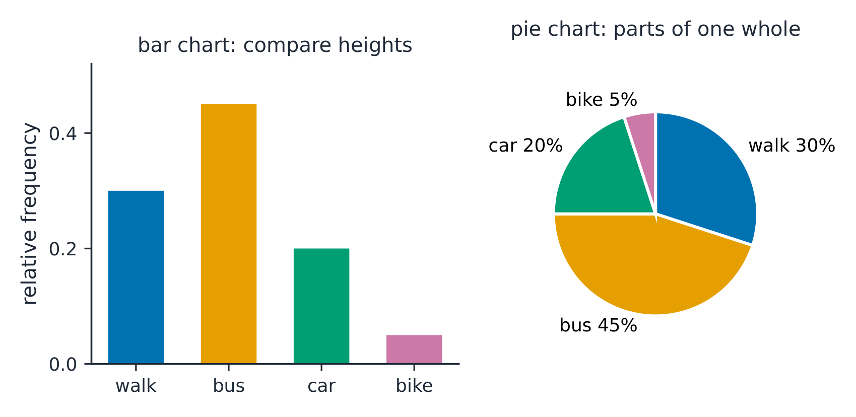
Bar charts 条形图 show the count or proportion of each category as separated bars; a pie chart shows each category's share of the whole. The bar heights (or slices) let you compare categories at a glance. Bars may be ordered by size or by a natural category order. On a bar chart the bars do not touch, and the order of the categories carries no meaning unless the categories have a natural order.
To compare two or more groups on the same categorical variable, use relative frequencies, not counts. A side-by-side bar graph 并列条形图 puts each group's bars next to each other. A segmented bar graph 分段条形图 gives each group one bar of height $1$ ($100\%$), divided into segments for the categories. If the segments are about the same size in every bar, the distribution of the variable is similar across the groups.
Explore
Show a categorical variable as a pie chart
A pie chart turns each category's share of the whole into a slice: a bigger share is a bigger slice, and every slice together makes 100%. It is a picture of a relative-frequency table.
Vocabulary
Train
| English |
|---|
| Bar charts/bɑː tʃɑːts/ |
| side-by-side bar graph |
| segmented bar graph |
1.5
Representing a Quantitative Variable with Graphs
Syllabus
| Enduring Understanding | Learning Objective | Essential Knowledge |
|---|---|---|
UNC-1 | UNC-1.F |
|
UNC-1.G |
|
Source: College Board AP Course and Exam Description
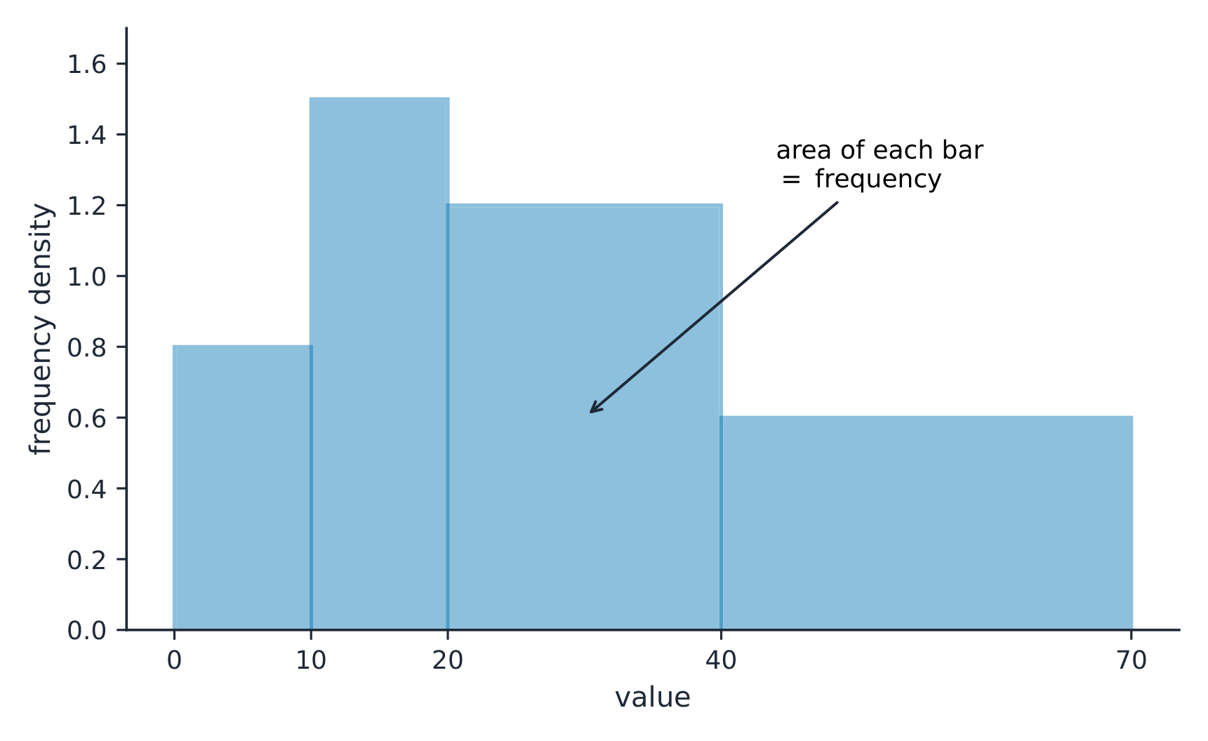
For numbers, use a dotplot 点图, stem-and-leaf plot 茎叶图, or histogram 直方图 (bars over value intervals called bins). These show the distribution 分布 – how the values spread out. A histogram's bin width changes the picture, so choose it to reveal the shape.
A discrete 离散 variable takes countable values, such as the number of siblings ($0,1,2,\dots$). A continuous 连续 variable can take any value in an interval, such as a time or a mass: between any two values there is always another. A dotplot places one dot per observation above a number line, stacking equal values. A stem-and-leaf plot splits each value into a stem (leading digits) and a leaf (last digit), so it keeps every data value: the stem $4$ with leaves $2\,5\,5\,8$ stands for $42, 45, 45, 48$. A cumulative graph plots the proportion of values at or below each value (see below).
Explore
Explore how bin width shapes a histogram
A histogram groups data into equal-width bins and draws a bar over each. Change the bins and notice how the same data can look jagged (too narrow) or smooth (too wide) — the shape is a choice.
Vocabulary
Train
| English |
|---|
| dotplot/ˈdɒtplɒt/ |
| stem-and-leaf plot/stem ænd liːf plɒt/ |
| histogram/ˈhɪstəɡræm/ |
| distribution/ˌdɪstrɪˈbjuːʃn/ |
| discrete/dɪˈskriːt/ |
| continuous/kənˈtɪnjuːəs/ |
1.6
Describing the Distribution of a Quantitative Variable
Syllabus
| Enduring Understanding | Learning Objective | Essential Knowledge |
|---|---|---|
UNC-1 | UNC-1.H |
|
Source: College Board AP Course and Exam Description
Describe four things (remember SOCS):
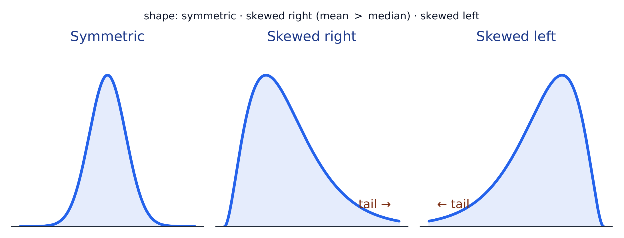
- Shape 形状: symmetric, or skewed 偏斜 left/right (a long tail on that side), and how many peaks - one main peak is unimodal 单峰, two prominent peaks bimodal 双峰, and roughly equal bars uniform 均匀.
- Outliers 离群值: unusual values far from the rest.
- Center: a typical value (mean or median).
- Spread: how much the values vary (range, IQR, standard deviation).
Always describe shape/center/spread in context, with units.
Common mistakes. Naming skew by the peak instead of the tail: a long tail to the left is skewed left, even though most values pile up on the right. Writing “the data are normal” from a histogram: say “roughly symmetric and unimodal”, because real data are only ever approximately normal. Leaving out context: “the median is $7$” earns less than “the median commute is $7$ minutes”.
Also look for gaps (stretches of the number line with no data) and clusters (groups of values separated by gaps). These often show that the data mix two kinds of individuals.
Worked example (describing a distribution). A dotplot shows the tips one waiter received on one day: most are between $\$2$ and $\$6$, with a long tail toward higher values and one tip of $\$18$. A full answer: "The distribution of tip amounts is skewed right, with a median of about $\$4$. Most tips lie between $\$2$ and $\$6$ (a range of about $\$16$ including the high tip). The $\$18$ tip appears to be an outlier." It names the shape, the centre, the spread and the unusual feature, all with units. A description like this is descriptive only: it is about this waiter's tips on this day, not every day.
Explore
Reading the shape
A long tail to one side means the distribution is skewed that way — skew is named for the tail.
Vocabulary
Train
| English |
|---|
| Shape/ʃeɪp/ |
| skewed/skjuːd/ |
| unimodal/ˌʌnɪˈmɒdl/ |
| bimodal/baɪˈmɒdl/ |
| uniform/ˈjuːnɪfɔːm/ |
| Outliers/ˈaʊtlaɪəz/ |
1.7
Summary Statistics for a Quantitative Variable
Syllabus
| Enduring Understanding | Learning Objective | Essential Knowledge |
|---|---|---|
UNC-1 | UNC-1.I |
|
UNC-1.J |
| |
UNC-1.K |
|
Source: College Board AP Course and Exam Description
- Center: the mean 均值 $\bar{x}=\dfrac{\sum x_i}{n}$ (average) and the median 中位数 (middle value). The median resists outliers; the mean is pulled toward a skew.
- Spread: the range, the interquartile range 四分位距 $\text{IQR}=Q_3-Q_1$ (middle 50%), and the standard deviation 标准差 $s_x=\sqrt{\dfrac{\sum(x_i-\bar{x})^2}{n-1}}$ (typical distance from the mean; its square is the variance 方差).
- The five-number summary 五数概括: min, $Q_1$, median, $Q_3$, max.
Use resistant measures (median, IQR) for skewed data; mean and standard deviation for roughly symmetric data. With an even number of values, the median is the mean of the two middle values.
What changes when one value changes? Suppose the $\$8$ tip in a set of tips had been $\$18$, and $\$8$ was already above the median. The mean goes up, because the sum grows by $\$10$. The standard deviation goes up, because that value is now farther from the mean. The median and the IQR do not change, because the middle values and the quartiles are the same values as before. The mean, the standard deviation and the range are nonresistant: one extreme value moves them.
Changing units. Adding the same constant to every value (for example, $+5$ points to every test score) shifts the mean, median and quartiles by that constant, but leaves the range, IQR and standard deviation unchanged. Multiplying every value by a positive constant (for example, converting metres to centimetres, $\times100$) multiplies all of them: the centre and the spread.
Worked example (combining groups). At one school, $200$ teachers have a mean of $9.1$ years' experience, and $18$ more teachers have a mean of $2.5$ years. The mean for all $218$ is not the mean of $9.1$ and $2.5$; weight each group by its size:
$$\bar x=\frac{200(9.1)+18(2.5)}{218}=\frac{1820+45}{218}=8.56\ \text{years}.$$
The percentile 百分位数 of a value is the percent of the data at or below it – so the median is the 50th percentile and $Q_1$ the 25th. A cumulative relative frequency graph 累积相对频率图 makes percentiles easy to read: for each value it plots the proportion of the data at or below it, rising from 0 to 1. Go up from a value to the curve and across to its percentile, or reverse the steps to find the value at a given percentile (the same reading works from a cumulative-frequency table).
Worked example. For the data $4, 8, 6, 10, 7$: the mean is $\bar{x}=\dfrac{4+8+6+10+7}{5}=\dfrac{35}{5}=7$. Sorting to $4,6,7,8,10$, the median is the middle value, $7$. The mean and median agree here because the data are roughly symmetric.
Worked example: standard deviation. For the same data, $\bar x=7$. Work in a table: each deviation from the mean, then its square.
| $x_i$ | $4$ | $6$ | $7$ | $8$ | $10$ |
|---|---|---|---|---|---|
| $x_i-\bar x$ | $-3$ | $-1$ | $0$ | $1$ | $3$ |
| $(x_i-\bar x)^2$ | $9$ | $1$ | $0$ | $1$ | $9$ |
The squares add to $20$. Divide by $n-1=4$, not by $n$, then take the square root:
$$s_x=\sqrt{\frac{\sum(x_i-\bar x)^2}{n-1}}=\sqrt{\frac{20}{4}}=\sqrt5\approx 2.24.$$
Interpretation: a typical value is about $2.24$ away from the mean of $7$. The deviations always add to $0$ (here $-3-1+0+1+3=0$), which is why they are squared first.
Common mistakes. Dividing by $n=5$ instead of $n-1=4$ (that gives $\sqrt4=2$, not $2.24$); stopping at the variance, $5$, and reporting it as the standard deviation; and describing $s_x$ as a distance from the median, or as the largest distance from the mean, instead of a typical distance from the mean.
Explore
Center and spread of data
The mean and median mark the center; the range, IQR, and standard deviation measure the spread.
Vocabulary
Train
| English |
|---|
| mean/miːn/ |
| median/ˈmiːdiːən/ |
| interquartile range/ˌɪntəˈkwɔːtaɪl reɪndʒ/ |
| standard deviation/ˈstændəd ˌdiːvɪˈeɪʃn/ |
| variance/ˈveərɪəns/ |
| five-number summary/faɪv ˈnʌmbə ˈsʌməri/ |
| percentile/pəˈsentaɪl/ |
| cumulative relative frequency graph/ˈkjuːmjʊlətɪv ˈrelətɪv ˈfriːkwənsi ɡræf/ |
1.8
Graphical Representations of Summary Statistics
Syllabus
| Enduring Understanding | Learning Objective | Essential Knowledge |
|---|---|---|
UNC-1 | UNC-1.L |
|
UNC-1.M |
|
Source: College Board AP Course and Exam Description
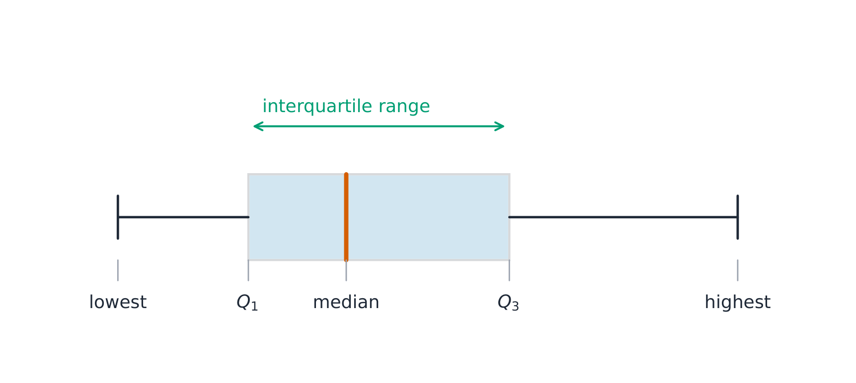
A boxplot 箱线图 draws the five-number summary: a box from $Q_1$ to $Q_3$ with the median inside, and whiskers to the most extreme non-outlier values. A point is an outlier if it lies more than $1.5\times\text{IQR}$ beyond a quartile – a rule you may be asked to apply. Boxplots are ideal for comparing several groups side by side.
Worked example. A dataset has $Q_1=20$ and $Q_3=32$, so $\text{IQR}=12$. The outlier fences are $Q_1-1.5(12)=2$ and $Q_3+1.5(12)=50$. Any value below $2$ or above $50$ is flagged as an outlier.
A second rule, also used in this course, flags a value that is 2 or more standard deviations from the mean. The two rules can disagree. In a strongly skewed data set the standard deviation is inflated by the long tail, so the $1.5\times\text{IQR}$ rule usually flags more points. If a question asks which rule identifies a value as an outlier, compute both fences and check.
Mean, median and shape. In a roughly symmetric distribution the mean and median are close together. In a right-skewed distribution the mean is usually to the right of (greater than) the median; in a left-skewed distribution, to the left.
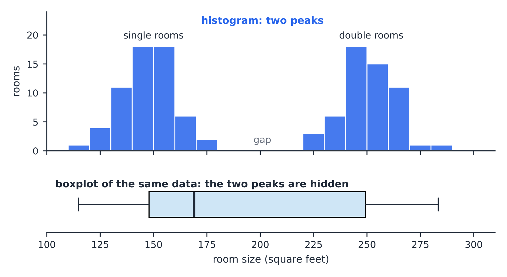
What a boxplot hides. A boxplot shows only five numbers. It cannot show peaks, gaps or clusters, so two very different distributions can have the same boxplot.
Common mistakes. Building the fences from the range instead of the IQR; adding $1.5\times\text{IQR}$ to the median instead of to the quartiles; and drawing a whisker out to the fence ($50$) instead of to the largest value that is not an outlier.

Explore
Explore the five-number summary as a boxplot
Drag $Q_1$, the median, and $Q_3$ to see the box (its length is the IQR) and how the median's position inside the box reveals skew — a median close to $Q_1$ signals a right-skewed distribution.
Vocabulary
Train
| English |
|---|
| boxplot/ˈbɒksplɒt/ |
1.9
Comparing Distributions of a Quantitative Variable

Syllabus
| Enduring Understanding | Learning Objective | Essential Knowledge |
|---|---|---|
UNC-1 | UNC-1.N |
|
UNC-1.O |
|
Source: College Board AP Course and Exam Description
To compare two or more groups, compare shape, center, and spread, and mention outliers – always with comparative words ("Group A has a higher median than Group B") and in context. Do not just describe each group separately; make the comparison explicit.
Worked example (comparing in context). Boxplots show yearly salaries at Corporation A (median $\$40{,}000$, IQR $\$12{,}000$, no outliers) and Corporation B (median $\$34{,}000$, IQR $\$20{,}000$, two high outliers). A strong answer: "The median salary at A ($\$40{,}000$) is higher than at B ($\$34{,}000$). Salaries at B are more variable: the IQR at B is $\$20{,}000$, compared with $\$12{,}000$ at A. Both are roughly symmetric, but B has two unusually high salaries." For a job offered at $\$36{,}000$, A might appeal because more of its salaries are high (its median is above the offer). B might appeal because a few people earn far more, and $\$36{,}000$ is already above B's median.
Explore
Compare distributions with box plots
A box plot draws the five-number summary. Placing two box plots on the same scale compares their centre (median), spread (IQR = box width) and skew at a glance — the fair way to compare groups.
1.10
The Normal Distribution
Syllabus
| Enduring Understanding | Learning Objective | Essential Knowledge |
|---|---|---|
VAR-2 | VAR-2.A |
|
VAR-2.B |
| |
VAR-2.C |
|
Source: College Board AP Course and Exam Description
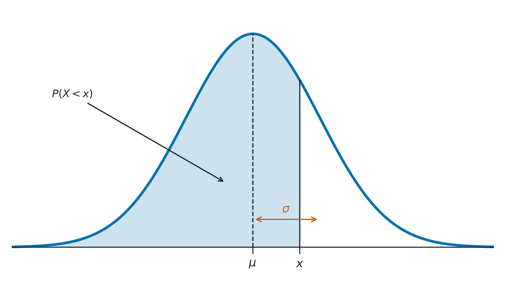
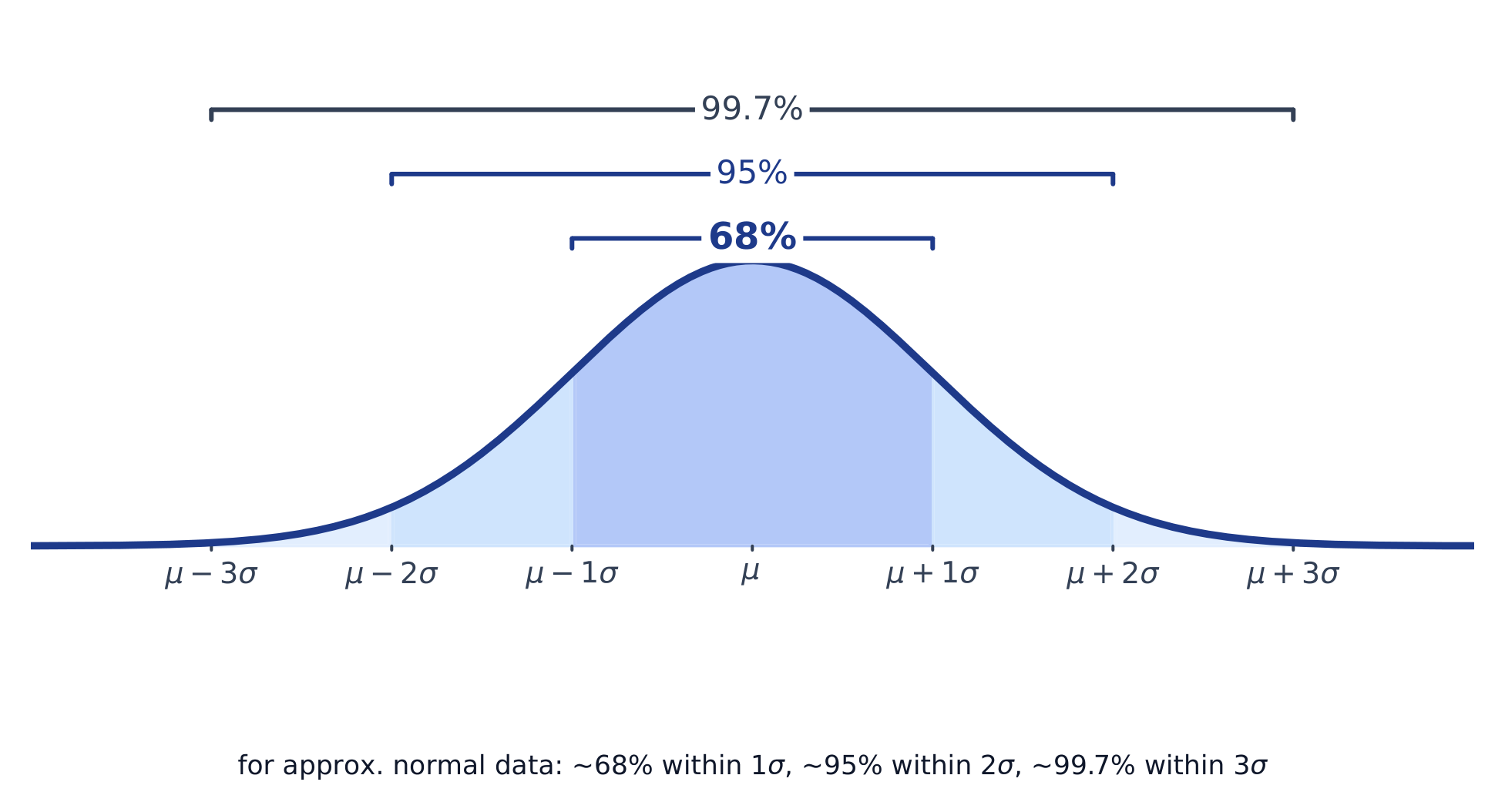
A normal distribution 正态分布 is a symmetric, bell-shaped model described by its mean $\mu$ and standard deviation $\sigma$. The empirical rule 经验法则 (68–95–99.7): about 68% of values lie within $1\sigma$ of the mean, 95% within $2\sigma$, and 99.7% within $3\sigma$.
A $z$-score 标准分数 measures how many standard deviations a value is from the mean:
$$z=\frac{x-\mu}{\sigma}.$$
Convert to a $z$-score, then use the normal table or technology to find the proportion (area) below, above, or between values – and reverse the process to find a value from a given percentile.
Worked example. Test scores are normal with $\mu=500$ and $\sigma=100$. A score of $700$ has $z=\dfrac{700-500}{100}=2$. By the empirical rule, $95\%$ of scores lie within $2\sigma$, so $2.5\%$ lie above $700$ – meaning a $700$ is at about the $97.5$th percentile.
Worked example: between two values, and backwards. With the same $\mu=500$, $\sigma=100$:
- Proportion between $450$ and $650$: $z=\dfrac{450-500}{100}=-0.5$ and $z=\dfrac{650-500}{100}=1.5$. The area is $P(z<1.5)-P(z<-0.5)=0.9332-0.3085=0.6247$, so about $62.5\%$ of scores.
- The score at the $90$th percentile: the table (or invNorm) gives $z=1.28$ for an area of $0.90$ below. Solve $z=\dfrac{x-\mu}{\sigma}$ for $x$: $x=\mu+z\sigma=500+1.28(100)\approx 628$.
Worked example (a percentile from the model). Battery life is normal with $\mu=30$ months and $\sigma=6$ months. After how many months have $25\%$ of batteries failed? That is the $25$th percentile: the table gives $z=-0.674$ for an area of $0.25$ below, so $x=30-0.674(6)=26.0$ months.
A $z$-score also compares values from different distributions. A score of $82$ on a test with mean $70$ and SD $8$ ($z=1.5$) is relatively better than $90$ on a test with mean $80$ and SD $10$ ($z=1.0$).
On the exam, show the distribution, the boundary and the area: “Normal, $\mu=500$, $\sigma=100$, $P(450<X<650)\approx 0.6247$”. A bare calculator command does not earn full credit.
Common mistakes. Using the empirical rule for a $z$-score that is not a whole number ($z=1.5$ needs the table or technology); giving the area below when the question asks for the proportion above (subtract from $1$); and using a normal model for a distribution the question describes as strongly skewed.
Explore
From a raw value to a normal-model area
$z=(x-\mu)/\sigma$
Connect the lesson’s raw values to standardised bounds and the correct shaded region. Changing a model does not show that real data follow it.
Vocabulary
Train
| English |
|---|
| normal distribution/ˈnɔːml ˌdɪstrɪˈbjuːʃn/ |
| empirical rule/emˈpɪrɪkl ruːl/ |
1.10
Practice
Answer each before reading the answers below.
-
For the data $3,\ 5,\ 7,\ 8,\ 9,\ 12,\ 15$, find the median and the IQR, and check for outliers with the $1.5\times IQR$ rule.
-
Household incomes in a city are strongly right-skewed. Which is larger, the mean or the median? Which better describes a typical household?
-
A test has mean 70 and standard deviation 8. Find the $z$-score of a student who scored 82.
-
If the scores in question 3 are approximately normal, what proportion of students scored below 58?
-
A student says: "The mean is always the best measure of center." Correct the student.
-
The $30$ values in a data set have mean $20$ and standard deviation $4$. Every value is multiplied by $3$ and then $5$ is added. Find the new mean and standard deviation.
-
A class of $12$ has a mean score of $78$, and another class of $18$ has a mean of $68$. Find the mean for all $30$ students.
-
A data set has $\bar x=50$, $s=5$, $Q_1=46$ and $Q_3=53$. Is a value of $61$ an outlier by the $1.5\times\text{IQR}$ rule? By the 2-standard-deviation rule?
1.10
Answers
-
Median $8$. $Q_1=5$ and $Q_3=12$ (medians of the lower and upper halves), so $IQR=7$. The fences are $5-10.5=-5.5$ and $12+10.5=22.5$; no value lies outside them, so there are no outliers.
-
The mean is larger, pulled up by the few very high incomes. The median better describes a typical household, because it resists extreme values.
-
$z=\dfrac{82-70}{8}=1.5$: one and a half standard deviations above the mean.
-
$z=\dfrac{58-70}{8}=-1.5$, so the proportion is about $0.067$, or $6.7\%$.
-
The mean is sensitive to outliers and skew. For skewed data or data with outliers, the median is the better summary of a typical value; report the IQR with it.
-
Mean: $3(20)+5=65$. Standard deviation: $3(4)=12$; adding $5$ does not change the spread.
-
$\dfrac{12(78)+18(68)}{30}=\dfrac{936+1224}{30}=72$.
-
$\text{IQR}=7$, so the upper fence is $53+10.5=63.5$: $61$ is not an outlier by that rule. It is $\dfrac{61-50}{5}=2.2$ standard deviations above the mean, so it is an outlier by the 2-SD rule.
1.10
Exam tips
- Describe a distribution by shape, center, spread, and outliers (SOCS) — always in context.
- The mean is pulled by outliers; the median resists them, so prefer the median for skewed data.
- For a normal distribution use the 68–95–99.7 rule and z-scores $z=\tfrac{x-\mu}{\sigma}$.
- Compare distributions with side-by-side boxplots and comment on center, spread, and shape.
- Standard deviation measures a typical distance from the mean; the IQR pairs with the median.
- When one value changes, say which statistics change and why: the mean and SD move; the median and IQR stay unless the middle of the data changes.
- Compare groups with proportions, not counts, when the groups differ in size.
Vocabulary
Train
| English |
|---|
| z-score/zed skɔː/ |
Interactive lessons on this topic
Work through it step by step, with instant-check exercises.
- Introducing Statistics: What Can We Learn from Data?
- The Language of Variation: Variables
- Representing a Categorical Variable with Tables
- Representing a Categorical Variable with Graphs
- Representing a Quantitative Variable with Graphs
- Describing the Distribution of a Quantitative Variable
- Summary Statistics for a Quantitative Variable
- Graphical Representations of Summary Statistics
- Comparing Distributions of a Quantitative Variable
- The Normal Distribution