| Enduring Understanding | Learning Objective | Essential Knowledge |
|---|---|---|
VAR-1 | VAR-1.J |
|
Inference for Categorical Data: Chi-Square
AP Statistics · Topic 8
 7:49
Inference for Categorical Data: Chi-Square
Roll a fair die sixty times. Every face should come up ten times. But it never does — eight here, thirteen there. The gaps are always there. So roll another…
English narration · English + 中文 subtitles burned in
8.1
Are My Results Unexpected?
Syllabus
Source: College Board AP Course and Exam Description
Do Grade 10 and Grade 11 students study in different places? Ask 200 of them and the counts will never split perfectly evenly, even if grade makes no difference at all. The question this unit answers is how uneven the counts must be before chance stops being a good explanation.
When data are counts 频数 spread across several categories 类别, we test whether the observed counts 观测频数 differ from what a claim predicts. The tool is the chi-square 卡方 ($\chi^2$) statistic, which adds up the standardized gaps between observed and expected counts:
$$\chi^2=\sum \frac{(\text{observed}-\text{expected})^2}{\text{expected}}.$$
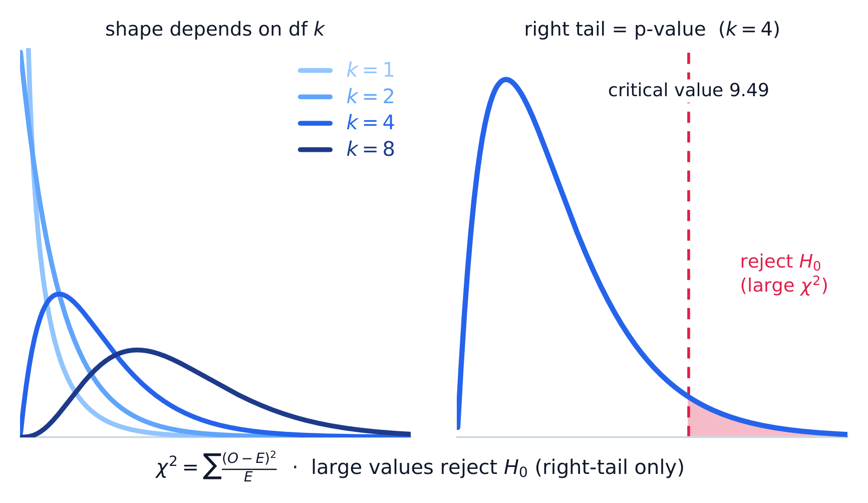
A large $\chi^2$ means the observed counts are far from expected – evidence against the claim. The chi-square distribution 卡方分布 is right-skewed 右偏的 and depends on its degrees of freedom 自由度.
Vocabulary
Train
| English |
|---|
| count |
| observed count |
| chi-square/kaɪ skweə/ |
| chi-square distribution |
| right-skewed |
| degrees of freedom/dɪˈɡriːz ɒv ˈfriːdəm/ |
8.2
Setting Up a Goodness-of-Fit Test
Syllabus
| Enduring Understanding | Learning Objective | Essential Knowledge |
|---|---|---|
VAR-8 | VAR-8.A |
|
VAR-8.B |
| |
VAR-8.C |
| |
VAR-8.D |
| |
VAR-8.E |
|
Source: College Board AP Course and Exam Description
A goodness-of-fit (GOF) 拟合优度 test checks whether one categorical variable 分类变量 follows a claimed distribution (e.g. "the die is fair"). Hypotheses:
$$H_0:\text{the distribution is as claimed}\qquad H_a:\text{at least one proportion differs}.$$
Expected count 期望频数 for each category $=n\times(\text{claimed proportion})$. Conditions 条件: random sample, all expected counts $\ge 5$, and the 10% condition.
Vocabulary
Train
| English |
|---|
| category/ˈkætɪɡəri/ |
| goodness-of-fit/ˈɡʊdnəs ɒv fɪt/ |
| categorical variable |
| expected count/ekˈspektɪd kaʊnt/ |
| conditions/kənˈdɪʃnz/ |
8.3
Carrying Out a Goodness-of-Fit Test
Syllabus
| Enduring Understanding | Learning Objective | Essential Knowledge |
|---|---|---|
VAR-8 | VAR-8.F |
|
VAR-8.G |
| |
DAT-3 | DAT-3.I |
|
DAT-3.J |
|
Source: College Board AP Course and Exam Description
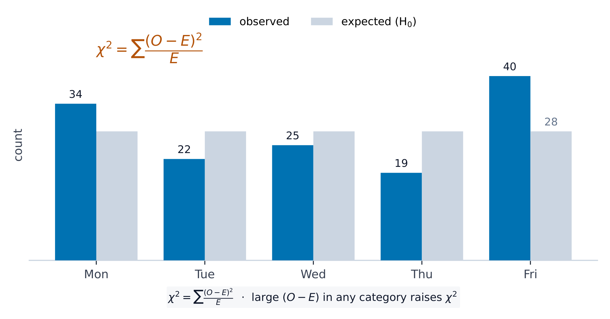
Compute $\chi^2=\sum\dfrac{(O-E)^2}{E}$ with $df=(\text{number of categories})-1$. Find the $p$-value P值 from the chi-square distribution (upper tail 右尾), compare to $\alpha$, and conclude in context. A large component of the sum points to the category that deviates most.
Worked example. A die rolled $60$ times gives counts $8,10,12,9,11,10$. If it is fair, each expected count is $60/6=10$, so
$$\chi^2=\frac{(8-10)^2}{10}+\frac{(10-10)^2}{10}+\frac{(12-10)^2}{10}+\frac{(9-10)^2}{10}+\frac{(11-10)^2}{10}+\frac{(10-10)^2}{10}=0.4+0+0.4+0.1+0.1+0=1.0,$$
with $df=6-1=5$. Write out every category, including the two that match their expected count exactly and so add $0$ – the sum runs over all six categories, and $df$ counts categories, not just the ones that differ. This $\chi^2$ is small (a large $p$-value), so we fail to reject 不拒绝 $H_0$ – no evidence the die is unfair.
Worked example: unequal claimed proportions. A sweet maker claims its bags are $30\%$ red, $20\%$ green and $50\%$ yellow. A random sample of $200$ sweets has $70$ red, $30$ green and $100$ yellow.
| Colour | Red | Green | Yellow |
|---|---|---|---|
| Observed | $70$ | $30$ | $100$ |
| Expected | $200(0.30)=60$ | $200(0.20)=40$ | $200(0.50)=100$ |
$$\chi^2=\frac{(70-60)^2}{60}+\frac{(30-40)^2}{40}+\frac{(100-100)^2}{100}=1.67+2.50+0=4.17,\qquad df=3-1=2.$$
The $p$-value is about $0.12>0.05$, so fail to reject $H_0$: there is not convincing evidence that the colour distribution differs from the maker's claim. The expected counts come from the claimed percentages, not from dividing $200$ equally by $3$.
Interpreting the $p$-value. "Assuming the colours really are $30\%$, $20\%$ and $50\%$, there is about a $0.12$ probability of getting a $\chi^2$ statistic of $4.17$ or larger in a random sample of $200$ sweets." The null distribution can be the $\chi^2$ model or a simulation of many samples from the claimed distribution; either gives the right-tail area beyond the observed statistic.
Explore
Explore the chi-square distribution and its p-value
The p-value is the area in the right tail beyond your test statistic, so a larger $\chi^2$ means a smaller p-value. Drag $\chi^2$ to watch that area shrink, and drag df to see the whole family change shape — strongly right-skewed at small df, more symmetric as df grows.
Vocabulary
Train
| English |
|---|
| upper tail |
| fail to reject/feɪl tə rɪˈdʒekt/ |
8.4
Expected Counts in Two-Way Tables
Syllabus
| Enduring Understanding | Learning Objective | Essential Knowledge |
|---|---|---|
VAR-8 | VAR-8.H |
|
Source: College Board AP Course and Exam Description
For a two-way table 双向表, the expected count in a cell (under "no association") is
$$E=\frac{(\text{row total})\times(\text{column total})}{\text{grand total}}.$$
This is the count you would see if the row and column variables were unrelated (no association 关联).
Worked example. In a two-way table a cell's row total is $40$, its column total is $50$, and the grand total is $200$. Its expected count is $E=\dfrac{40\times50}{200}=10$. Repeating for every cell gives the expected table to compare against the observed one.

Vocabulary
Train
| English |
|---|
| two-way table/tuː weɪ ˈteɪbl/ |
| association/əˌsəʊsɪˈeɪʃn/ |
8.5
Homogeneity or Independence?
Syllabus
| Enduring Understanding | Learning Objective | Essential Knowledge |
|---|---|---|
VAR-8 | VAR-8.I |
|
VAR-8.J |
| |
VAR-8.K |
|
Source: College Board AP Course and Exam Description
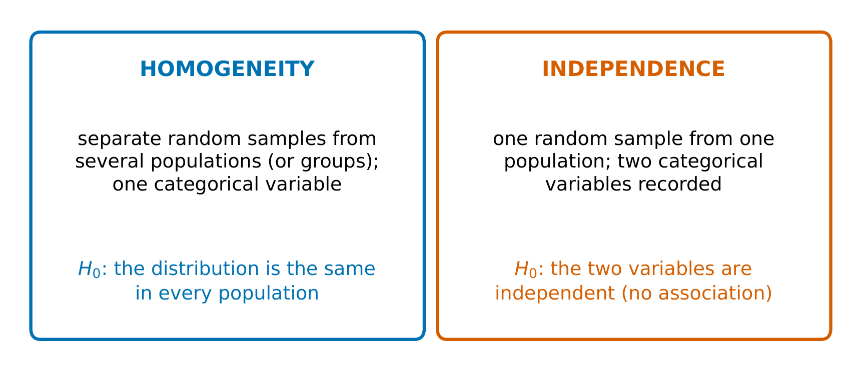
Two tests use the same $\chi^2$ math but answer different questions:
- Test for homogeneity 同质性检验: are the distributions of one categorical variable the same across several populations or groups (separate samples/treatments)?
- Test for independence 独立性检验: are two categorical variables associated within a single population (one sample, two variables measured)?
The design (several samples vs one sample) decides which name and hypotheses to use.
Writing the hypotheses. For homogeneity, the null says the proportions in each category are the same in every group. For three cities and one yes/no question: $H_0:p_A=p_B=p_C$, where each $p$ is the proportion of all teens in that city who drank a soft drink in the past week; $H_a$: at least two of these proportions differ. For independence: $H_0$: there is no association between the two variables in the population; $H_a$: there is an association.
Experiments. A randomized experiment with a categorical response is analysed with the same chi-square test for homogeneity: the treatment groups play the part of the populations. If children are randomly assigned to watch one of three ads and then choose a snack, a small $p$-value is evidence that the type of ad causes a difference in snack choice, for children similar to those in the study.
Vocabulary
Train
| English |
|---|
| test for homogeneity/test fɔː ˈhɒməʊdʒneɪti/ |
| test for independence/test fɔː ˌɪndɪˈpendəns/ |
8.6
Carrying Out a Test for Homogeneity or Independence
Syllabus
| Enduring Understanding | Learning Objective | Essential Knowledge |
|---|---|---|
VAR-8 | VAR-8.L |
|
VAR-8.M |
| |
DAT-3 | DAT-3.K |
|
DAT-3.L |
|
Source: College Board AP Course and Exam Description
Compute expected counts, then $\chi^2=\sum\dfrac{(O-E)^2}{E}$ over all cells, with
$$df=(\text{rows}-1)(\text{columns}-1).$$
Conditions: random data, all expected counts $\ge 5$, 10% condition. Find the $p$-value, compare to $\alpha$, and conclude in context – evidence of a difference between groups (homogeneity) or of an association (independence).
Worked example: a test for independence. A random sample of 200 students at one school is classified by grade and by where they usually study.
| Library | Home | Café | Total | |
|---|---|---|---|---|
| Grade 10 | 30 | 50 | 20 | 100 |
| Grade 11 | 45 | 35 | 20 | 100 |
| Total | 75 | 85 | 40 | 200 |
- State. $H_0$: grade and study place are independent for students at this school. $H_a$: they are associated.
- Plan. Chi-square test for independence: one sample, two variables. Random sample; 200 is less than 10% of the students if the school has more than 2000; expected counts below are all at least 5.
- Do. Expected counts: $\dfrac{100\times75}{200}=37.5$, then $42.5$ and $20$ in each row. The six components are $1.50,\ 1.32,\ 0,\ 1.50,\ 1.32,\ 0$, so $\chi^2=5.65$ with $df=(2-1)(3-1)=2$, giving $p\approx0.059$.
- Conclude. Because $p\approx0.059>\alpha=0.05$, fail to reject $H_0$. There is not convincing evidence of an association between grade and study place for students at this school.
The library cells contribute most: Grade 11 students chose the library more often than expected. That is worth noting as a pattern, but with this $p$-value it is not convincing evidence.
Common mistakes. Checking the condition with observed counts: it is the expected counts that must all be at least $5$. Running chi-square on percentages or means instead of counts. Using $df=n-1=199$ instead of $(r-1)(c-1)=2$. Writing the conclusion about the sample ("these students are associated") instead of the population the sample represents.
Is the test appropriate? Before any chi-square test, compute the smallest expected count. If a table of athletes has a cell with expected count $\tfrac{12\times18}{80}=2.7$, the large-counts condition fails, so the $\chi^2$ $p$-value would not be reliable. Collect more data, or combine categories in a sensible way (for example, merge two small age groups) until every expected count is at least $5$. Writing $H_0$ as “grade and study place are associated”: the null hypothesis always says no association. Calling a one-sample, two-variable test “homogeneity”.
8.7
Choosing the Right Categorical Procedure
Syllabus
This topic is intended to focus on the skill of selecting an appropriate inference procedure now that students have a range of options. Students should be given opportunities to practice when and how to apply all learning objectives relating to inference for categorical data.
Source: College Board AP Course and Exam Description
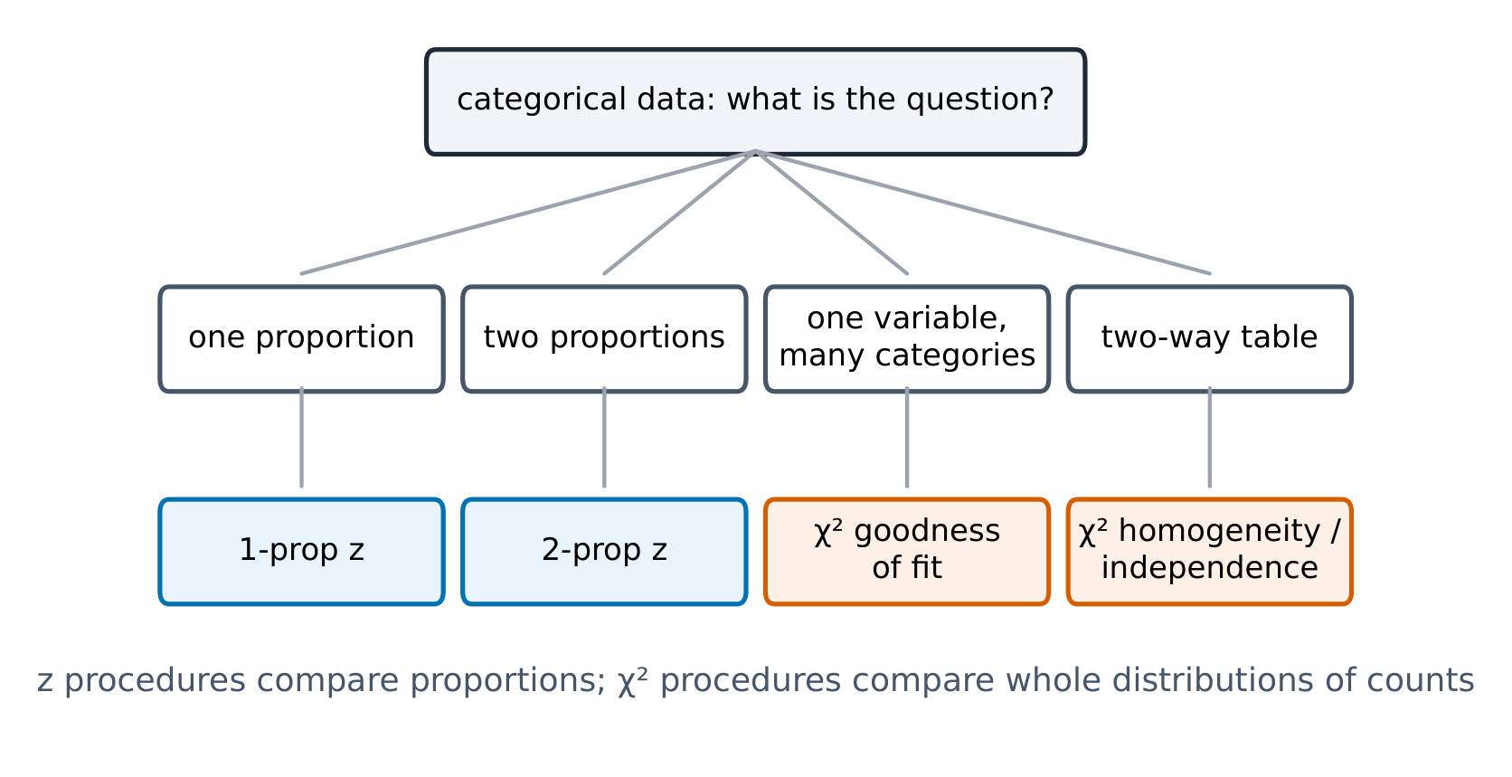
Decide by the setup: one categorical variable against a claimed distribution $\Rightarrow$ goodness-of-fit; one sample cross-classified by two variables $\Rightarrow$ independence; several samples/groups compared $\Rightarrow$ homogeneity. Comparing just two proportions can use either a two-proportion $z$-test or a chi-square test, but only for a two-tailed 双尾 alternative, where they agree exactly ($\chi^2=z^2$). The chi-square statistic is compared with the upper tail of its reference distribution. For two proportions it tests a non-directional alternative, so if $H_a$ is one-sided 单侧 (say $p_1>p_2$), use the $z$-test.
Explore
Which chi-square test is this?
All three tests use the same $\chi^2$ arithmetic, so the marks are won by naming the right one. The design decides — how many samples were taken, and how many variables were measured on each unit.
Vocabulary
Train
| English |
|---|
| two-tailed/tuː teɪld/ |
| one-sided |
8.7
Practice
Answer each before reading the answers below.
-
In a two-way table, a cell's row total is 60, its column total is 50 and the grand total is 200. Find its expected count.
-
A two-way table has 3 rows and 4 columns. Find the degrees of freedom for a chi-square test.
-
A die is rolled 60 times, giving counts $6,\ 10,\ 8,\ 12,\ 14,\ 10$ for faces 1 to 6. Find $\chi^2$ for a goodness-of-fit test of a fair die. Its $p$-value is about $0.55$. Conclude.
-
Name the test: (a) one random sample of 500 adults, classified by phone brand and age group; (b) separate random samples from three cities, comparing favourite sport; (c) the colours in a bag of sweets, compared with the maker's claimed percentages.
-
A student says: “In the worked example $p=0.059$, so grade and study place are independent.” Correct the student.
-
A randomized experiment assigns $150$ patients to three treatments and records whether each improves. Name the test and write its hypotheses.
-
A two-way table has row totals $30$ and $70$, column totals $15$, $40$ and $45$, and grand total $100$. Is a chi-square test appropriate? Check the smallest expected count.
8.7
Answers
-
$\dfrac{60\times50}{200}=15$.
-
$(3-1)(4-1)=6$.
-
Each expected count is 10. $\chi^2=\dfrac{16+0+4+4+16+0}{10}=4.0$, $df=5$. With $p\approx0.55$, fail to reject $H_0$: no convincing evidence that the die is unfair.
-
(a) Independence; (b) homogeneity; (c) goodness-of-fit.
-
Failing to reject $H_0$ means the data are not convincing evidence of an association. It does not prove independence: a real but small association could still exist. Write “not convincing evidence of an association”, never “they are independent”.
-
A chi-square test for homogeneity. $H_0$: the proportion of patients who improve is the same for all three treatments; $H_a$: at least two of the proportions differ. With random assignment, a significant result supports a cause-and-effect conclusion.
-
Smallest expected count $=\tfrac{30\times15}{100}=4.5<5$, so the condition fails and the chi-square test is not appropriate as it stands.
8.7
Exam tips
- Use $\chi^2=\sum\tfrac{(O-E)^2}{E}$ for categorical data; always divide by the expected count.
- Pick the right test: goodness-of-fit (one variable), independence, or homogeneity (two-way table).
- Compute expected counts as $\tfrac{\text{row total}\times\text{column total}}{\text{grand total}}$ and check each is $\ge5$.
- A large $\chi^2$ (small p-value) means observed counts differ from expected by more than chance.
- State degrees of freedom correctly (categories $-1$, or $(r-1)(c-1)$).
- Before testing, find the smallest expected count; if it is below $5$, the chi-square test is not appropriate.
- Write the conclusion about the population (or the treatments), never just about the sample.
Vocabulary
Train
| English |
|---|
| p-value/piː ˈvæljuː/ |
Interactive lessons on this topic
Work through it step by step, with instant-check exercises.