| Enduring Understanding | Learning Objective | Essential Knowledge |
|---|---|---|
VAR-1 | VAR-1.D |
|
Exploring Two-Variable Data
AP Statistics · Topic 2
 7:49
Exploring Two-Variable Data
Thirty children from one primary school. For each child, two numbers: shoe size, and a reading test score. Plot one point per child. The pattern is hard to…
English narration · English + 中文 subtitles burned in
2.1
Are Two Variables Related?
Syllabus
Source: College Board AP Course and Exam Description
Do students who take more semesters to graduate earn higher starting salaries? Do children choose fruit more often after a healthy-food advert? A newspaper may claim a link from a handful of people. This unit gives you the tools to check: tables and graphs to see a pattern, $r$ to measure it, and a regression line to predict with it.
Two-variable data let us ask whether two characteristics are associated 关联 – whether knowing one tells you something about the other. An explanatory variable 解释变量 (the "input") may help predict a response variable 响应变量 (the "output"). Association is not the same as causation. Also, a pattern in a sample may be random: with few individuals, chance alone can produce an apparent association that would vanish in more data. Units 4 to 9 show how to judge whether a pattern is larger than chance would produce.
Vocabulary
Train
| English |
|---|
| associated/əˈsəʊsɪeɪtɪd/ |
| explanatory variable/ekˈsplænətəri ˈveərɪəbl/ |
| response variable/rɪˈspɒns ˈveərɪəbl/ |
2.2
Two Categorical Variables
Syllabus
| Enduring Understanding | Learning Objective | Essential Knowledge |
|---|---|---|
UNC-1 | UNC-1.P |
|
Source: College Board AP Course and Exam Description
A two-way table 双向表 (contingency table) counts individuals by two categorical variables at once. A marginal distribution 边缘分布 is a row or column total written as a fraction of the grand total (the totals themselves are just counts). Comparing the inside cells shows whether the variables are related. A joint relative frequency 联合相对频率 is one cell divided by the grand total: the proportion of all individuals who are in that row and that column.
Explore
A categorical breakdown
Each slice is one category's share of the whole.
Vocabulary
Train
| English |
|---|
| two-way table/tuː weɪ ˈteɪbl/ |
| marginal distributions/ˈmɑːdʒɪnl ˌdɪstrɪˈbjuːʃnz/ |
| joint relative frequency |
2.3
Comparing Groups with Conditional Distributions

Syllabus
| Enduring Understanding | Learning Objective | Essential Knowledge |
|---|---|---|
UNC-1 | UNC-1.Q |
|
UNC-1.R |
|
Source: College Board AP Course and Exam Description
A conditional distribution 条件分布 is the distribution of one variable within a fixed category of the other (found by dividing each cell by its row or column total). If the conditional distributions differ across groups, the two variables are associated; if they are the same, there is no association. Segmented bar charts 分段条形图 or mosaic plots display them. A mosaic plot 马赛克图 is a segmented bar graph whose bar widths are proportional to the group sizes, so it shows the marginal and the conditional distributions at once.
Worked example. A school records how $200$ students took a course and whether they passed.
| Passed | Failed | Total | |
|---|---|---|---|
| Online | $60$ | $40$ | $100$ |
| In person | $75$ | $25$ | $100$ |
| Total | $135$ | $65$ | $200$ |
- Marginal distribution of result: $\tfrac{135}{200}=0.675$ passed and $\tfrac{65}{200}=0.325$ failed.
- Conditional distributions: online students passed at $\tfrac{60}{100}=0.60$; in-person students at $\tfrac{75}{100}=0.75$.
The conditional pass rates differ ($0.60$ vs $0.75$), so the format and the result are associated in these data. This alone does not show that the format causes the difference: students chose their format.
Divide by the correct total: “the proportion of online students who passed” uses the online total ($100$), while “the proportion of passes that were online” uses the pass total: $\tfrac{60}{135}\approx 0.44$.
Three proportions from the table above, for the same cell:
- joint: $\tfrac{60}{200}=0.30$ of all students were online and passed;
- conditional on format: $\tfrac{60}{100}=0.60$ of online students passed;
- conditional on result: $\tfrac{60}{135}=0.44$ of students who passed were online.
When the FRQ asks you to "describe the effect" of a factor, compare conditional proportions across the groups and give the numbers.
Vocabulary
Train
| English |
|---|
| conditional distribution/kənˈdɪʃənl ˌdɪstrɪˈbjuːʃn/ |
| Segmented bar charts/seɡˈmentɪd bɑː tʃɑːts/ |
| mosaic plot |
2.4
Scatterplots for Two Quantitative Variables

Syllabus
| Enduring Understanding | Learning Objective | Essential Knowledge |
|---|---|---|
UNC-1 | UNC-1.S |
|
DAT-1 | DAT-1.A |
|
Source: College Board AP Course and Exam Description
A scatterplot 散点图 plots each individual as a point, explanatory variable on the $x$-axis and response on the $y$-axis. Describe it with DUFS: Direction (positive/negative), Unusual features (outliers, clusters), Form (linear or curved), and Strength (how tightly the points follow the pattern) – always in context.
Worked example. A scatterplot shows height and arm span for $12$ seniors. A full description: "There is a strong, positive, linear association between height and arm span for these seniors: taller seniors tend to have longer arm spans. There are no obvious outliers." Use "tend to": the pattern describes the group, not every pair of points.
Explore
A scatterplot with a linear trend
Drag to see how direction and strength change the cloud of points.
Vocabulary
Train
| English |
|---|
| scatterplot/ˈskætəplɒt/ |
2.5
Correlation

Syllabus
| Enduring Understanding | Learning Objective | Essential Knowledge |
|---|---|---|
DAT-1 | DAT-1.B |
|
DAT-1.C |
|
Source: College Board AP Course and Exam Description
The correlation coefficient 相关系数 $r$ measures the strength and direction of a linear relationship. It runs from $-1$ to $1$: near $\pm 1$ is strong linear, near $0$ is weak linear. $r$ has no units and does not change if you swap the variables. Warnings: $r$ only measures linear strength, it is not resistant to outliers, and a strong $r$ does not prove causation.
How $r$ is built. Change each $x$ and $y$ to a $z$-score, multiply the pairs, and average (dividing by $n-1$):
$$r=\frac{1}{n-1}\sum\left(\frac{x_i-\bar x}{s_x}\right)\left(\frac{y_i-\bar y}{s_y}\right).$$
Points in the upper-right and lower-left (both $z$-scores of the same sign) add positive products; points in the other two corners add negative ones. Because it uses $z$-scores, $r$ does not change if you change units (inches to centimetres) or add a constant to every value. $r=\pm1$ only when all points lie exactly on a line. A value of $r$ near $\pm1$ does not by itself show that a line is the right model: a smooth curve can also have $r=0.95$.
Explore
Strength of a linear relationship
Correlation $r$ runs from $-1$ to $1$: near $\pm1$ the points hug a line, near 0 they scatter. Change it and watch the cloud tighten or spread.
Vocabulary
Train
| English |
|---|
| correlation coefficient/ˌkɒrɪˈleɪʃn ˌkəʊɪˈfɪʃənt/ |
2.6
Linear Regression Models

Syllabus
| Enduring Understanding | Learning Objective | Essential Knowledge |
|---|---|---|
DAT-1 | DAT-1.D |
|
Source: College Board AP Course and Exam Description
The least-squares regression line 最小二乘回归线 predicts the response: $\hat{y}=a+bx$, where $\hat{y}$ is the predicted response. The slope 斜率 $b$ is the predicted change in $y$ per one-unit increase in $x$; the $y$-intercept 纵截距 $a$ is the predicted $y$ when $x=0$. Interpret both in context and with units – a graded skill. Avoid extrapolation 外推 (predicting far outside the data).
From summary statistics, the line comes from two formulas: the slope is $b=r\,\dfrac{s_y}{s_x}$, and the line always passes through $(\bar x,\bar y)$, so $a=\bar y-b\bar x$.
Worked example. A study of hours studied ($x$) and test score ($y$) gives $\hat{y}=20+3x$. The slope means each extra hour of study is associated with a predicted $3$-point increase. A student who studies $5$ hours is predicted to score $\hat{y}=20+3(5)=35$. The intercept says a student who studies $0$ hours is predicted to score $20$. Sometimes the intercept has no sensible meaning: a car of length $0$ inches, or a house of $0$ square metres, does not exist.
Worked example: line from summary statistics. For another class, hours studied have $\bar x=6$ and $s_x=2$; scores have $\bar y=70$ and $s_y=10$; and $r=0.8$.
$$b=r\,\frac{s_y}{s_x}=0.8\times\frac{10}{2}=4, \qquad a=\bar y-b\bar x=70-4(6)=46.$$
So $\hat y=46+4x$: each extra hour is associated with a predicted $4$-point increase. Also $r^2=0.64$: $64\%$ of the variation in scores is explained by the linear relationship with hours studied.
Reading computer output. Exams often give regression output instead of an equation.
| Predictor | Coef | SE Coef | T | P |
|---|---|---|---|---|
| Constant | $12.40$ | $3.10$ | $4.00$ | $0.001$ |
| Semesters | $1.85$ | $0.42$ | $4.40$ | $0.000$ |
$S = 3.61\quad$ R-Sq $= 54.2\%$
The Constant row gives the intercept and the row named after the explanatory variable gives the slope: $\widehat{\text{salary}}=12.40+1.85(\text{semesters})$, in thousands of dollars. Interpretation of the slope: "For each extra semester, the predicted starting salary increases by about $\$1850$." $S$ is the standard deviation of the residuals: predictions are typically off by about $\$3610$. R-Sq is $r^2$. Since the slope is positive, $r=+\sqrt{0.542}=0.74$. (The SE, T and P columns are for inference in unit 9.)
Explore
Fit a least-squares line
A regression line is the best straight-line fit, minimising the squared vertical distances. Its slope predicts how $y$ changes per unit of $x$.
Vocabulary
Train
| English |
|---|
| least-squares regression line/liːst skweəz rɪˈɡreʃn laɪn/ |
| slope/sləʊp/ |
| y-intercept/waɪ ˌɪntəˈsept/ |
| extrapolation/ekˈstræpəleɪʃn/ |
2.7
Residuals

Syllabus
| Enduring Understanding | Learning Objective | Essential Knowledge |
|---|---|---|
DAT-1 | DAT-1.E |
|
DAT-1.F |
|
Source: College Board AP Course and Exam Description
A residual 残差 is actual minus predicted, $y-\hat{y}$: how far a point sits above (+) or below (−) the line. A residual plot 残差图 graphs residuals against $x$. If it shows no pattern (random scatter), a linear model is appropriate; a curved or fanning pattern means the linear model is a poor fit.
Worked example. Continuing the study above, a student who studied $5$ hours actually scored $40$. The residual is $y-\hat{y}=40-35=+5$: the line under-predicted by $5$ points, so this point sits above the line. In context: "The student scored $5$ points higher than the line predicts for a student who studied $5$ hours." A residual close to $0$ means the line predicted that individual's response almost exactly.
A residual plot can put the residuals against $x$ or against the predicted values $\hat y$; both are read the same way. Look for curves (wrong form) and a fan shape (the spread of the residuals grows with $x$, so predictions are less reliable for large $x$).
Common mistakes. Computing predicted minus actual ($35-40=-5$): a residual is always actual minus predicted. Stating the slope as a certainty (“the score goes up by $3$”) instead of a predicted change, or without units and context. Interpreting the intercept when $x=0$ lies far outside the data.
Explore
Residuals = vertical gaps to the line
Each point's vertical distance from the line is its residual.
Vocabulary
Train
| English |
|---|
| residual/rɪˈsɪdʒuːəl/ |
| residual plot/rɪˈsɪdʒuːəl plɒt/ |
2.8
Least-Squares Regression and Its Fit

Syllabus
| Enduring Understanding | Learning Objective | Essential Knowledge |
|---|---|---|
DAT-1 | DAT-1.G |
|
DAT-1.H |
|
Source: College Board AP Course and Exam Description
The line minimizes the sum of squared residuals. Its fit is measured by:
- $s$, the standard deviation of the residuals – the typical prediction error, in the response's units.
- $r^2$, the coefficient of determination 决定系数 – the proportion of the variation in $y$ that the linear model explains (a value between $0$ and $1$; multiply by $100$ to state it as a percent). Report it in context: “$r^2 = 0.81$ means 81% of the variation in $y$ is explained by the linear relationship with $x$.”
Common mistakes. Saying $r=0.8$ means “$80\%$ of the variation is explained”: that statement belongs to $r^2=0.64$. Calling $r\approx0$ “no relationship”: a strong curve can have $r$ near $0$. Saying a high $r$ or $r^2$ shows a linear model is right: only the residual plot shows that.
Explore
The best-fit least-squares line
The line that makes the total squared vertical gap smallest.
Vocabulary
Train
| English |
|---|
| coefficient of determination/ˌkəʊɪˈfɪʃənt ɒv dɪˌtɜːmɪˈneɪʃn/ |
2.9
Departures from Linearity
Syllabus
| Enduring Understanding | Learning Objective | Essential Knowledge |
|---|---|---|
DAT-1 | DAT-1.I |
|
DAT-1.J |
|
Source: College Board AP Course and Exam Description
Some points strongly affect the line. A high-leverage 高杠杆 point has an extreme $x$-value; an influential 有影响的 point noticeably changes the slope or $r$ when removed; an outlier here is a point with a large residual. When the pattern is curved, transform a variable (e.g. take a log) to straighten it, then fit a line to the transformed data.
Worked example (an influential point). Ten countries give a weak positive scatter with $r=0.30$. An eleventh country has an $x$-value far beyond the others, and it lies on the upward trend. Adding it pulls the line toward it and raises $r$ to $0.75$. This point has high leverage (extreme $x$) and is influential (it changes the slope and $r$ a lot), even though its residual is small. A point with a large residual but an ordinary $x$-value is an outlier, and it usually changes the slope much less.
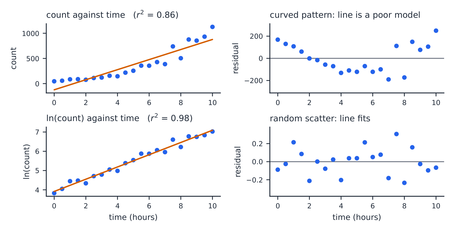
Worked example (a transformation). A bacteria count grows quickly with time. The straight line for count against time has $r^2=0.86$, but its residual plot is a clear U-shape, so the linear model is wrong. Taking $\ln(\text{count})$ gives a residual plot with no pattern and $r^2=0.98$. More random residuals and an $r^2$ closer to $1$ are evidence that the transformed model fits better. Predict with it, then undo the log: if $\widehat{\ln(\text{count})}=3.9+0.32t$, then at $t=5$, $\widehat{\ln(\text{count})}=5.5$ and the predicted count is $e^{5.5}\approx245$.
Explore
An influential point swings the line
A far-out point off the trend can tilt the whole line.
Vocabulary
Train
| English |
|---|
| high-leverage/haɪ ˈliːvərɪdʒ/ |
| influential/ˌɪnfluːˈenʃl/ |
2.9
Practice
Answer each before reading the answers below.
-
Of 120 students, 50 play a sport, and 30 of those 50 are also in a music group. What proportion of sport players are in a music group?
-
A scatterplot of hours slept against reaction time gives $r=-0.85$. Describe the relationship.
-
A regression line is $\hat y=12+2.5x$. Predict $y$ when $x=8$, and find the residual for a point $(8,\ 29)$.
-
The data in question 3 have $x$ values from 0 to 10. Why is predicting $y$ at $x=40$ risky?
-
A student says: “The correlation is $0.9$, so $x$ causes $y$.” Correct the student.
-
Computer output for predicting fuel use (litres per $100\ \text{km}$) from car length (inches) shows Constant $=-2.50$, Length $=0.0478$, R-Sq $=49.0\%$. Write the equation, and find and interpret the residual for a car $175$ inches long that uses $5.88$ litres per $100\ \text{km}$.
-
A data set has $r=0.6$. Every $x$-value is converted from inches to centimetres. What happens to $r$ and to the slope?
-
In a two-way table of $400$ voters, $90$ are under $30$ and support a proposal, and $150$ are under $30$ in total. Find the joint relative frequency of "under 30 and supports", and the proportion of under-30 voters who support.
2.9
Answers
-
$30/50=0.60$. This is a conditional proportion: it uses only the sport players as the whole.
-
A strong, negative, linear relationship: students who sleep more tend to have shorter reaction times.
-
$\hat y=12+2.5(8)=32$. Residual $=y-\hat y=29-32=-3$; the point lies 3 units below the line.
-
That is extrapolation: the pattern is known only for $x$ from 0 to 10, and nothing guarantees it continues to 40.
-
Correlation measures the strength of a linear association, not causation. A lurking variable could drive both, or the link could run the other way. Only a randomized experiment supports a cause-and-effect claim.
-
$\hat y=-2.50+0.0478x$. At $x=175$: $\hat y=-2.50+8.365=5.865$. Residual $=5.88-5.865=0.015$: the car uses only about $0.015$ litre per $100\ \text{km}$ more than predicted, so the line predicts it almost exactly.
-
$r$ stays $0.6$ ($r$ has no units). The slope is divided by $2.54$, because each centimetre is a smaller step in $x$ than each inch.
-
Joint: $\tfrac{90}{400}=0.225$. Conditional: $\tfrac{90}{150}=0.60$.
2.9
Exam tips
- On a scatterplot describe direction, form, strength, and outliers; $r$ ranges $-1$ to $1$.
- Correlation is not causation — a lurking variable can drive both.
- Interpret the slope of the least-squares line in context (“per one unit of $x$, predicted $y$ changes by $b$”).
- Check a residual plot: no pattern means a line fits; a curve means it does not. Avoid extrapolation.
- $r^2$ is the fraction of variation in $y$ explained by the model.
- Read the slope from the row named after the explanatory variable in computer output, and the intercept from Constant; $r$ takes the sign of the slope.
- Choose between models by the residual plot first, then $r^2$.
Interactive lessons on this topic
Work through it step by step, with instant-check exercises.