| Enduring Understanding | Learning Objective | Essential Knowledge |
|---|---|---|
VAR-1 | VAR-1.G |
|
Sampling Distributions
AP Statistics · Topic 5
 7:32
Sampling Distributions
Two thousand students go to this school, and some of them cycle here. We want to know what share. Nobody can ask all two thousand, so we ask a random hundred.…
English narration · English + 中文 subtitles burned in
5.1
Why Two Samples Never Match: Sampling Variability
Syllabus
Source: College Board AP Course and Exam Description
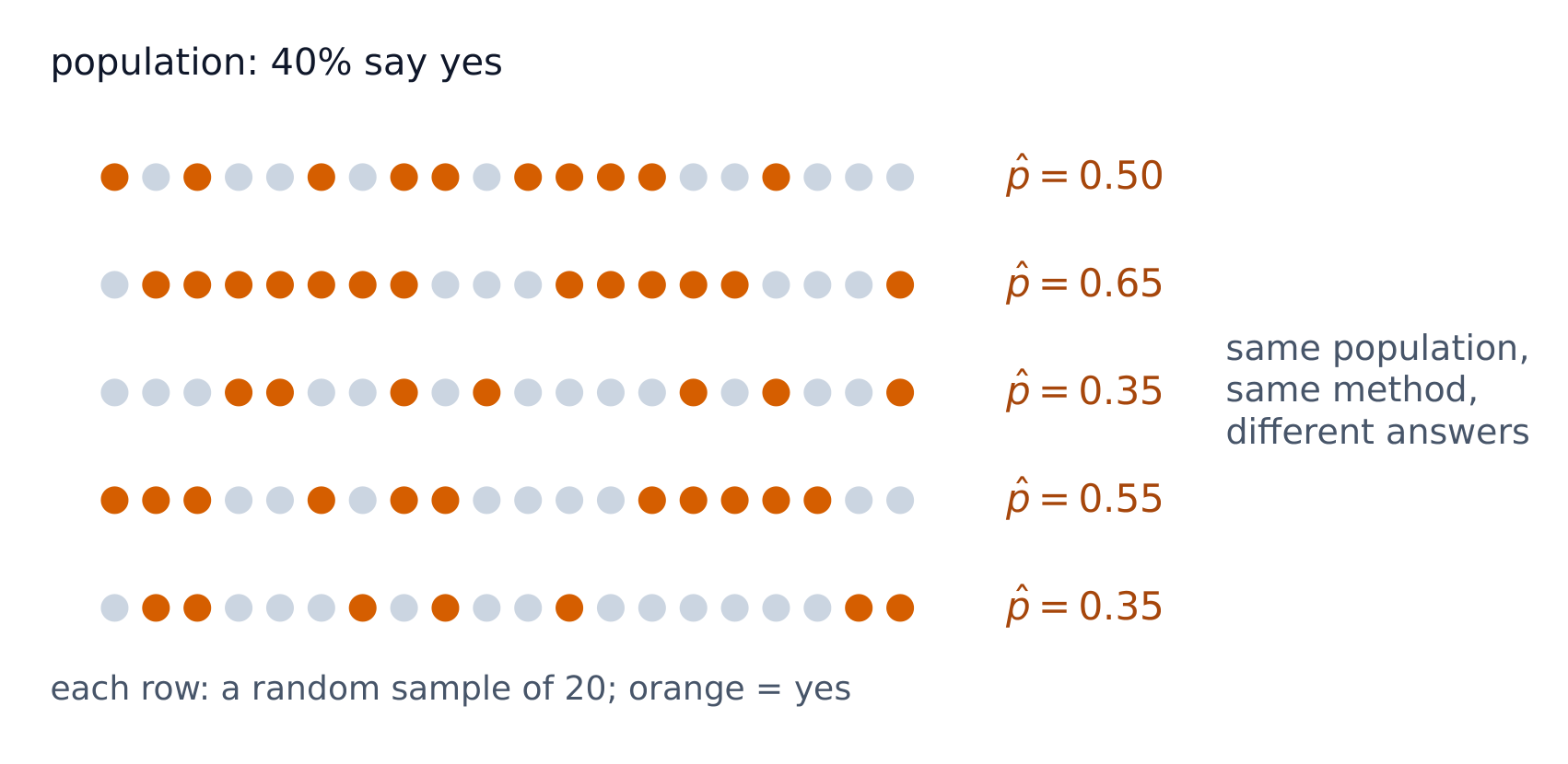
You and a friend each survey $50$ random students about the canteen. You find $62\%$ like it; your friend finds $54\%$. Neither of you made a mistake: random samples simply differ. How much they differ is predictable, and that prediction is the key to every confidence interval and test in the rest of the course.
A statistic 统计量 (like a sample mean 样本均值 $\bar{x}$ or sample proportion 样本比例 $\hat{p}$) is computed from a sample and varies from sample to sample – this is sampling variability 抽样变异性. A parameter 参数 ($\mu$ or $p$) is the fixed truth about the population 总体. The sampling distribution 抽样分布 is the distribution of a statistic over all possible samples of a given size – it is the bridge from one sample to inference 推断. Differences between samples can be random (sampling variability) or not (for example, one sample was chosen badly). The sampling distribution tells you how large the random differences usually are.
Vocabulary
Train
| English |
|---|
| statistic/stəˈtɪstɪk/ |
| sample mean/ˈsæmpl miːn/ |
| sample proportion/ˈsæmpl prəˈpɔːʃn/ |
| sampling variability/ˈsæmplɪŋ ˌveərɪəˈbɪlɪti/ |
| parameter/pəˈræmɪtə/ |
| population/ˌpɒpjʊˈleɪʃn/ |
| sampling distribution/ˈsæmplɪŋ ˌdɪstrɪˈbjuːʃn/ |
| inference/ˈɪnfərəns/ |
5.2
The Normal Curve as a Model for a Statistic
Syllabus
| Enduring Understanding | Learning Objective | Essential Knowledge |
|---|---|---|
VAR-6 | VAR-6.A |
|
VAR-6.B |
| |
VAR-6.C |
|
Source: College Board AP Course and Exam Description
For large enough samples, many sampling distributions are approximately normal 正态的. That lets us describe a statistic by a center 中心 (its mean), a spread 离散程度 (its standard error 标准误), and a normal shape – and then compute how likely a given sample result is.
A continuous random variable 连续随机变量 can take any value in an interval. Its probabilities are areas under a density curve, so the probability of any single exact value is $0$, and $P(X<a)=P(X\le a)$. To find an area, write the inequality for the interval, change the boundaries to $z$-scores, and use a table or technology. Normal models also work well for real distributions that are roughly symmetric and mound-shaped.
Explore
Use the normal curve to find a proportion
A normal model turns a range of values into an area = a proportion. Shade a band to read off the fraction of samples falling within it (the 68-95-99.7 rule).
Vocabulary
Train
| English |
|---|
| normal/ˈnɔːml/ |
| center/ˈsentə/ |
| spread/spred/ |
| standard error/ˈstændəd ˈerə/ |
| continuous random variable/kənˈtɪnjuːəs ˈrændəm ˈveərɪəbl/ |
5.3
The Central Limit Theorem
Syllabus
| Enduring Understanding | Learning Objective | Essential Knowledge |
|---|---|---|
UNC-3 | UNC-3.H |
|
Source: College Board AP Course and Exam Description
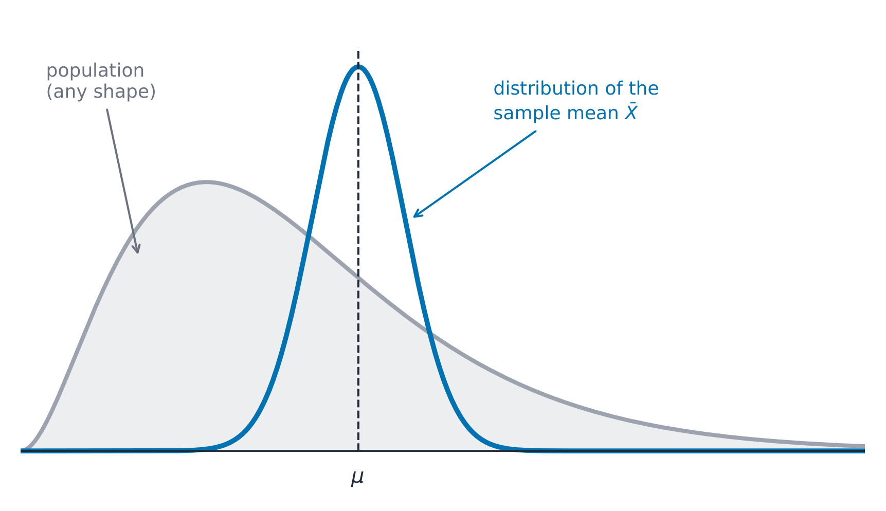
The Central Limit Theorem 中心极限定理 (CLT): for independent 独立 observations from the same population with finite, positive variance 方差, the sampling distribution of a sample mean becomes approximately normal as $n$ increases. A strongly skewed 偏斜 population may need a much larger sample than $30$; there is no universal sample-size cutoff. The standard error decreases as $n$ increases.
A sampling distribution can also be simulated: take many random samples from a population (or a model of it) and compute the statistic for each one. In a randomized experiment, a randomization distribution 随机化分布 is built the same way, by re-randomizing the units to groups many times as if the treatment had no effect, and recording the difference each time.
Explore
Raw observations and repeated sample means
$E(\bar X)=\mu,\quad \mathrm{SD}(\bar X)=\sigma/\sqrt n$
The population stays the same while the distribution of sample means changes. These are illustrative independent models; a large n does not make raw data normal.
Vocabulary
Train
| English |
|---|
| Central Limit Theorem/ˈsentrəl ˈlɪmɪt ˈθɪərəm/ |
| independent/ˌɪndɪˈpendənt/ |
| variance/ˈveərɪəns/ |
| skewed/skjuːd/ |
| randomization distribution |
5.4
Good Guesses and Bad Guesses: Bias
Syllabus
| Enduring Understanding | Learning Objective | Essential Knowledge |
|---|---|---|
UNC-3 | UNC-3.I |
|
UNC-3.J |
|
Source: College Board AP Course and Exam Description
A statistic is unbiased 无偏 if the mean of its sampling distribution equals the parameter – it is correct on average. Bias 偏差 is about the center being off; variability 变异性 is about the spread. A good estimator 估计量 is both unbiased (centered right) and low-variability (precise 精确的); larger samples reduce variability but do not fix bias from bad sampling. Any sample statistic used to estimate a parameter is a point estimate 点估计; its sampling distribution shows how far from the parameter it tends to land.
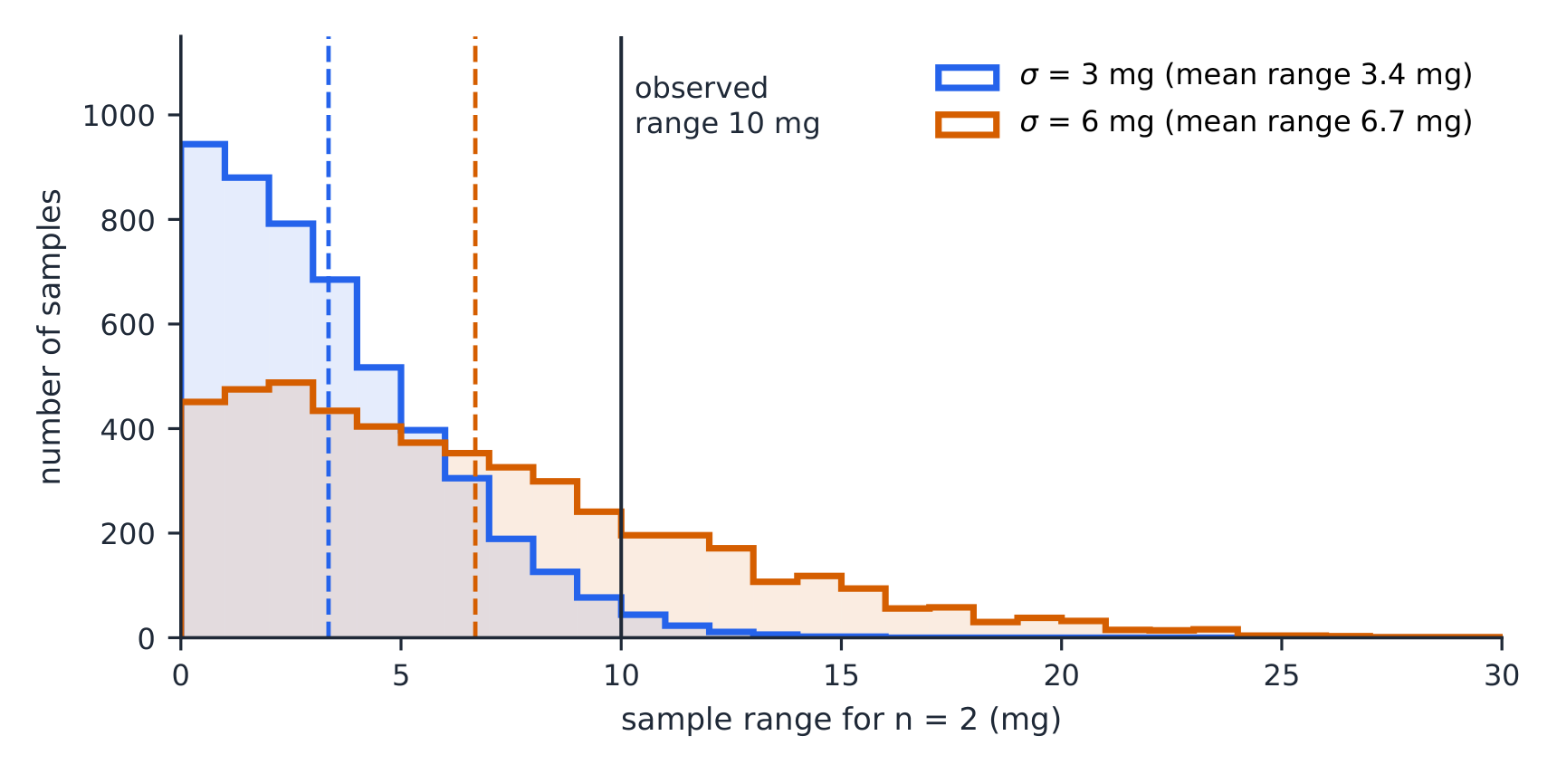
Other statistics. Every statistic has a sampling distribution, not only $\bar x$ and $\hat p$. The sample median is not always unbiased for the population mean (for a skewed population it is centred on the population median). The sample range of small samples is biased low (a sample rarely contains the most extreme values), and its distribution is skewed right.
Worked example (the sample range). A machine puts gold on necklaces; the amount is normal with $\mu=300\ \text{mg}$. A statistician measures $2$ necklaces a day and records the range. The figure shows $5000$ simulated ranges for $\sigma=3\ \text{mg}$ and for $\sigma=6\ \text{mg}$. As $\sigma$ grows, the distribution of the range shifts to the right and spreads out. A range of $10\ \text{mg}$ happens in under $2\%$ of samples when $\sigma=3$, but in about a quarter of them when $\sigma=6$: so an observed range of $10\ \text{mg}$ is evidence that $\sigma$ is larger than $3\ \text{mg}$.

Vocabulary
Train
| English |
|---|
| unbiased/ʌnˈbaɪəst/ |
| Bias/ˈbaɪəs/ |
| variability/ˌveərɪəˈbɪlɪti/ |
| estimator |
| precise/prɪˈsaɪs/ |
| point estimate/pɔɪnt ˈestɪmət/ |
5.5
The Sampling Distribution of a Sample Proportion

Syllabus
| Enduring Understanding | Learning Objective | Essential Knowledge |
|---|---|---|
UNC-3 | UNC-3.K |
|
UNC-3.L |
| |
UNC-3.M |
|
Source: College Board AP Course and Exam Description
For a sample proportion $\hat{p}$ from an SRS 简单随机样本: the mean is $p$ (unbiased), and the standard deviation 标准差 is
$$\sigma_{\hat p}=\sqrt{\frac{p(1-p)}{n}}.$$
This spread is the standard error: the standard deviation of the statistic's sampling distribution. When $p$ is unknown, replace it by $\hat p$ to estimate that standard error, as in the later inference units.
It is approximately normal when $np\ge 10$ and $n(1-p)\ge 10$ (the Large Counts condition 大计数条件), and the $10\%$ condition ($n\le 0.10N$) keeps the observations near-independent. Strictly, sampling without replacement makes the standard deviation a little smaller than the formula gives; when $n$ is under $10\%$ of the population, the difference is too small to matter.
Worked example (a point estimate). In a random sample of $300$ students, $87$ say yes. The point estimate of the population proportion is $\hat p=\tfrac{87}{300}=0.29$. Interpret the standard deviation in context: if $p$ were $0.29$, sample proportions from samples of $300$ would typically differ from $0.29$ by about $\sqrt{0.29(0.71)/300}=0.026$.
Worked example. Suppose $40\%$ of voters favor a measure ($p=0.4$) and you sample $n=100$. The standard error is $\sigma_{\hat p}=\sqrt{\dfrac{0.4(0.6)}{100}}=0.049$. The chance a sample gives $\hat{p}>0.5$ is $z=\dfrac{0.5-0.4}{0.049}=2.04$, so $P(\hat p>0.5)\approx0.02$ – a majority in the sample would be surprising.
Common mistakes. Checking “$n\ge30$” for a proportion: that rule belongs to means; for $\hat p$ check $np\ge10$ and $n(1-p)\ge10$ (here $40$ and $60$). Treating the $10\%$ condition as a normality check: it keeps the observations close to independent, so the formula for $\sigma_{\hat p}$ is valid.
Vocabulary
Train
| English |
|---|
| SRS |
| standard deviation/ˈstændəd ˌdiːvɪˈeɪʃn/ |
| Large Counts condition/lɑːdʒ kaʊnts kənˈdɪʃn/ |
5.6
Comparing Two Groups: Difference of Sample Proportions
Syllabus
| Enduring Understanding | Learning Objective | Essential Knowledge |
|---|---|---|
UNC-3 | UNC-3.N |
|
UNC-3.O |
| |
UNC-3.P |
|
Source: College Board AP Course and Exam Description
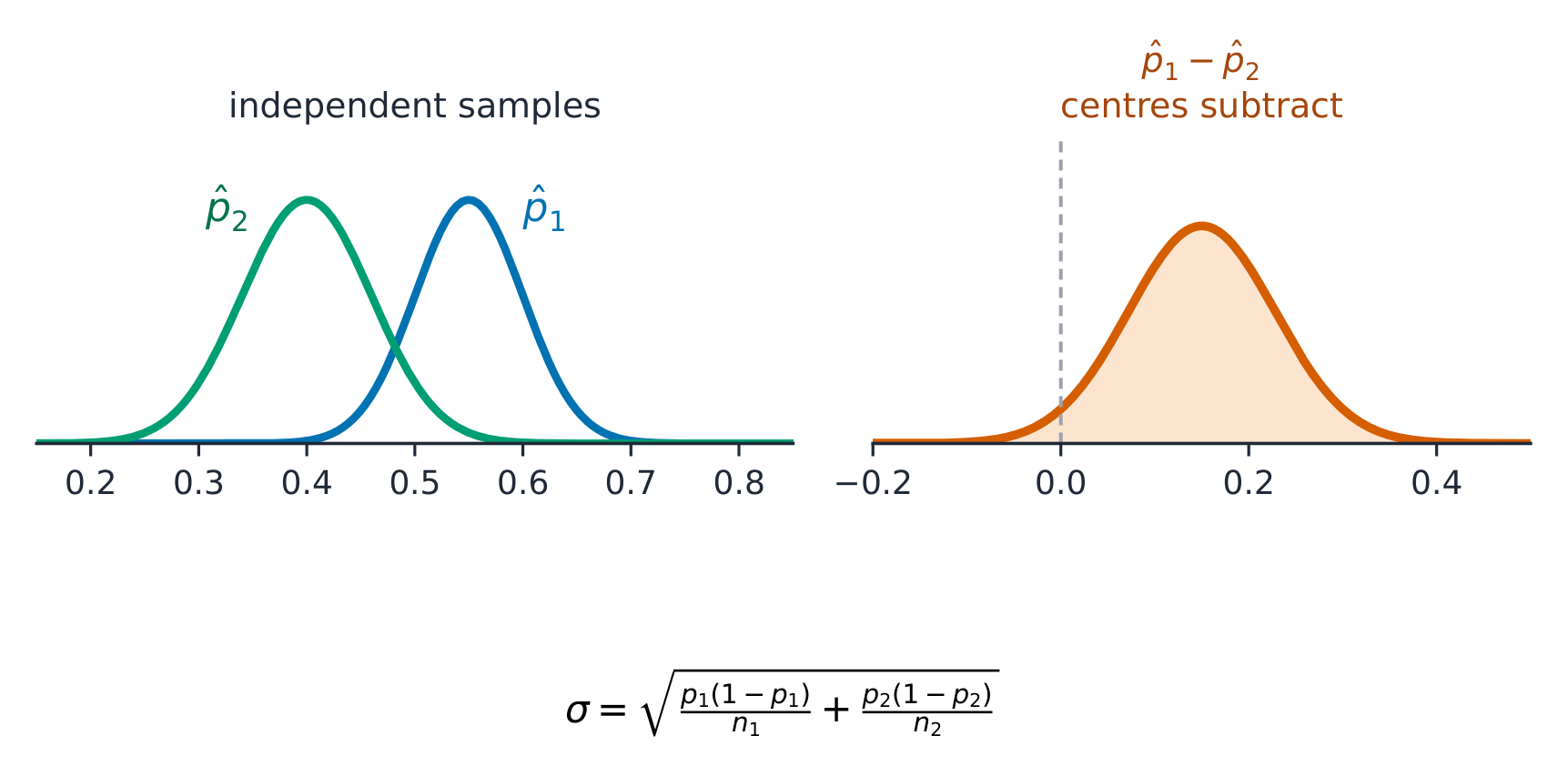
For $\hat{p}_1-\hat{p}_2$ from two independent samples: the mean is $p_1-p_2$, and because the samples are independent the variances add 方差相加:
$$\sigma_{\hat p_1-\hat p_2}=\sqrt{\frac{p_1(1-p_1)}{n_1}+\frac{p_2(1-p_2)}{n_2}}.$$
It is approximately normal when the Large Counts condition holds in both samples.
Worked example. In town 1, $60\%$ of adults cycle to work; in town 2, $50\%$. Independent random samples of $100$ adults are taken from each town. How likely is it that the town 1 sample shows a lower proportion than town 2?
The mean of $\hat p_1-\hat p_2$ is $0.6-0.5=0.10$, and
$$\sigma_{\hat p_1-\hat p_2}=\sqrt{\frac{0.6(0.4)}{100}+\frac{0.5(0.5)}{100}}=\sqrt{0.0049}=0.07.$$
Large Counts: $60$, $40$, $50$ and $50$ are all at least $10$, so use a normal model. $z=\dfrac{0-0.10}{0.07}\approx-1.43$, so $P(\hat p_1-\hat p_2<0)\approx 0.077$. About $8\%$ of such pairs of samples would put town 1 behind, even though town 1 really is ahead.
Vocabulary
Train
| English |
|---|
| variances add |
5.7
The Sampling Distribution of a Sample Mean

Syllabus
| Enduring Understanding | Learning Objective | Essential Knowledge |
|---|---|---|
UNC-3 | UNC-3.Q |
|
UNC-3.R |
| |
UNC-3.S |
|
Source: College Board AP Course and Exam Description
For a sample mean $\bar{x}$ from an SRS: the mean is $\mu$ (unbiased), and the standard deviation is
$$\sigma_{\bar x}=\frac{\sigma}{\sqrt{n}}.$$
Its shape is normal if the population is normal, or approximately normal for large $n$ by the CLT. Note the spread shrinks like $\sqrt{n}$ – quadrupling the sample halves the standard error. The spread of the data in one sample does not shrink with $n$: a sample of $200$ tortillas has about the same spread of diameters ($\approx\sigma$) as a sample of $20$. What shrinks is the spread of the sample means from one day to the next.
Worked example (three days instead of one). A school's daily absences are normal with $\mu=120$ and $\sigma=11$. It loses funding if absences on a randomly chosen day exceed $140$: $z=\tfrac{140-120}{11}=1.82$, so $P\approx0.034$. If the state instead uses the mean of $3$ randomly chosen days (assume independent), $\sigma_{\bar x}=\tfrac{11}{\sqrt3}=6.35$ and $z=\tfrac{140-120}{6.35}=3.15$, so $P\approx0.0008$. Averaging several days makes an extreme result much less likely.
Worked example. A population has $\mu=70$ and $\sigma=12$. For samples of $n=36$, the sampling distribution of $\bar{x}$ is centered at $70$ with standard error $\dfrac{12}{\sqrt{36}}=2$. The chance a sample mean exceeds $73$ is $z=\dfrac{73-70}{2}=1.5$, so $P(\bar x>73)\approx0.067$.
Common mistakes. Using $\sigma=12$ instead of $\sigma_{\bar x}=2$ for a question about a mean of $36$ values. For one individual, $z=(73-70)/12=0.25$ and $P(X>73)\approx0.40$: a single value above $73$ is common, a sample mean above $73$ is not. Saying the CLT makes the population (or the sample) normal: it is the sampling distribution of $\bar x$ that becomes approximately normal.
Explore
Individual spread and sample-mean spread
$\mathrm{SD}(\bar X)=\sigma/\sqrt n$
Changing n changes the standard error, not the population standard deviation. Normal probabilities require an explicit distribution model.
5.8
Comparing Two Groups: Difference of Sample Means
Syllabus
| Enduring Understanding | Learning Objective | Essential Knowledge |
|---|---|---|
UNC-3 | UNC-3.T |
|
UNC-3.U |
| |
UNC-3.V |
|
Source: College Board AP Course and Exam Description
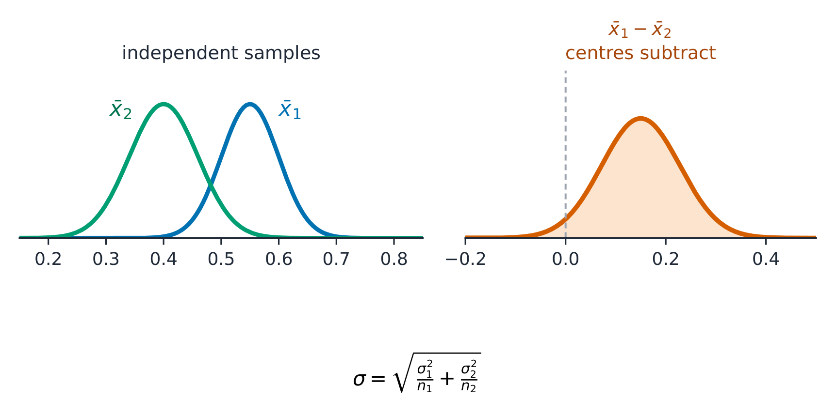
For $\bar{x}_1-\bar{x}_2$ from two independent samples: the mean is $\mu_1-\mu_2$, and (independent, so variances add)
$$\sigma_{\bar x_1-\bar x_2}=\sqrt{\frac{\sigma_1^2}{n_1}+\frac{\sigma_2^2}{n_2}}.$$
This is the foundation for two-sample inference in the next units.
Worked example. Machine 1 fills bottles with $\mu_1=500\ \text{mL}$ and $\sigma_1=4\ \text{mL}$; machine 2 with $\mu_2=498\ \text{mL}$ and $\sigma_2=3\ \text{mL}$. Both fill amounts are normal. Independent random samples of $16$ bottles from machine 1 and $9$ from machine 2 are taken. The mean of $\bar x_1-\bar x_2$ is $500-498=2\ \text{mL}$, and
$$\sigma_{\bar x_1-\bar x_2}=\sqrt{\frac{4^2}{16}+\frac{3^2}{9}}=\sqrt{1+1}\approx1.41\ \text{mL}.$$
Both populations are normal, so the difference is normal even for these small samples. The machine 2 sample has the larger mean when $\bar x_1-\bar x_2<0$:
$$z=\frac{0-2}{1.41}\approx-1.41,\qquad P(\bar x_1-\bar x_2<0)\approx0.079.$$
The variances add even though the means subtract: $1+1$ under the square root, never $1-1$.
5.8
Practice
Answer each before reading the answers below.
-
A population proportion is $p=0.30$ and samples of $n=50$ are taken. Give the mean and standard deviation of $\hat p$, and check the Large Counts condition.
-
A population has $\mu=100$ and $\sigma=15$. For samples of $n=25$, find $P(\bar x>106)$.
-
By what factor must the sample size grow to halve the standard deviation of $\bar x$?
-
A population of incomes is strongly right-skewed. Is $\bar x$ approximately normal for samples of $n=5$? For $n=50$?
-
A student says: "A bigger sample removes bias." Correct the student.
-
Heights of a plant species are normal with $\mu=40\ \text{cm}$ and $\sigma=6\ \text{cm}$. Find the probability that one plant is taller than $43\ \text{cm}$, and that the mean of $9$ plants is more than $43\ \text{cm}$.
-
Explain why the sample maximum is a biased estimator of the population maximum.
5.8
Answers
-
Mean $0.30$; standard deviation $\sqrt{0.30(0.70)/50}=0.065$. Large Counts: $np=15$ and $n(1-p)=35$, both at least 10.
-
$\sigma_{\bar x}=15/\sqrt{25}=3$, so $z=\dfrac{106-100}{3}=2.0$ and $P(\bar x>106)\approx0.023$.
-
Four times as large, because $\sigma_{\bar x}=\sigma/\sqrt n$.
-
Not for $n=5$: with a skewed population, a small sample's mean is still skewed. For $n=50$, probably yes: $n\ge 30$ is the usual AP guideline, so by the Central Limit Theorem $\bar x$ is approximately normal. An extremely skewed population (a few huge incomes) could still need a larger sample.
-
A larger sample reduces variability (the spread of the sampling distribution), not bias (where its center sits). A biased method such as a voluntary-response 自愿回应 poll stays biased, however large.
-
One plant: $z=\tfrac{43-40}{6}=0.5$, $P\approx0.309$. Mean of $9$: $\sigma_{\bar x}=\tfrac{6}{3}=2$, $z=1.5$, $P\approx0.067$.
-
A sample can never contain a value larger than the population maximum, and it usually misses the largest values, so the sample maximum is usually below the true maximum. Its sampling distribution is centred below the parameter, so it is biased (low).
Vocabulary
Train
| English |
|---|
| voluntary-response |
5.8
Exam tips
- A sampling distribution describes a statistic over repeated samples. It is centered on the true parameter when the statistic is unbiased.
- The Central Limit Theorem: for a large enough sample the sample mean is approximately normal, even if the population is not.
- Larger samples give less variability (a smaller standard error).
- Check the conditions (random, independent/10%, large enough) before using a normal model.
- Keep straight what varies — the statistic — versus the fixed parameter.
- Distinguish the spread of individual values ($\sigma$) from the spread of sample means ($\sigma/\sqrt n$); read which one the question asks about.
- To judge a sample result, place it in the sampling distribution: a value far in the tail is unlikely if the claimed parameter is true.
Interactive lessons on this topic
Work through it step by step, with instant-check exercises.