| Enduring Understanding | Learning Objective | Essential Knowledge |
|---|---|---|
VAR-1 | VAR-1.I |
|
Inference for Quantitative Data: Means
AP Statistics · Topic 7
 7:38
Inference for Quantitative Data: Means
You already know the heart of inference. Take a sample, find its mean, then do it again and again. Even when the population is lopsided, those sample means…
English narration · English + 中文 subtitles burned in
7.1
Should I Worry About Error?
Syllabus
Source: College Board AP Course and Exam Description
Inference for a mean 均值 works like inference for a proportion, with one change: we rarely know the population standard deviation 总体标准差 $\sigma$, so we estimate it with the sample $s$. That extra uncertainty means we use the $t$-distribution t分布 instead of the normal – a distribution 分布 that is bell-shaped but with heavier tails, and it depends on the degrees of freedom 自由度 $df=n-1$; as $n$ grows it approaches the normal.
A packing machine is supposed to fill bags of chips with $28.0\ \text{g}$. A quality checker weighs 20 bags and finds a mean of $27.4\ \text{g}$. Is the machine underfilling, or is $0.6\ \text{g}$ just the luck of which bags were picked? This unit turns that question into a number, and makes you say what could go wrong with your answer.
Vocabulary
Train
| English |
|---|
| mean/miːn/ |
| population standard deviation |
| distribution/ˌdɪstrɪˈbjuːʃn/ |
| degrees of freedom/dɪˈɡriːz ɒv ˈfriːdəm/ |
7.2
Confidence Interval for a Mean

Syllabus
| Enduring Understanding | Learning Objective | Essential Knowledge |
|---|---|---|
VAR-7 | VAR-7.A |
|
UNC-4 | UNC-4.O |
|
UNC-4.P |
| |
UNC-4.Q |
| |
UNC-4.R |
Boundary statement: Formulas for interval estimates do not appear explicitly on the AP Statistics Formula Sheet provided with the AP Statistics Exam. However, these formulas do not need to be memorized, as they can be constructed based on the general test statistic formula and the relevant standard error formulas that are provided on the formula sheet. |
Source: College Board AP Course and Exam Description
A one-sample $t$ confidence interval 置信区间 for $\mu$:
$$\bar{x}\pm t^{*}\frac{s}{\sqrt{n}}.$$
$t^{*}$ is the critical value 临界值 with $df=n-1$. Conditions: random sample, Normal/Large Sample (population normal, or $n\ge 30$ by the CLT, or a roughly symmetric sample with no outliers 异常值), and the 10% condition. Interpret the interval and the confidence level 置信水平 in context.
Worked example. A random sample of $n=25$ has $\bar{x}=50$ and $s=8$. For a $95\%$ interval, $df=24$ gives $t^*=2.064$:
$$50\pm2.064\cdot\frac{8}{\sqrt{25}}=50\pm2.064(1.6)=50\pm3.3=(46.7,\ 53.3).$$
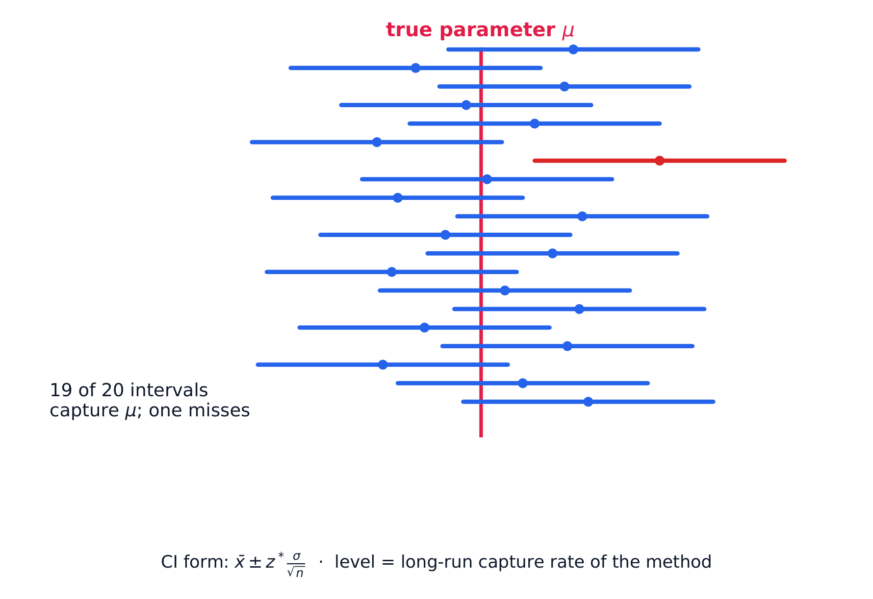
Interpretation: "We are $95\%$ confident that the interval from $46.7$ to $53.3$ captures the true mean of the population the sample was taken from." Name the variable and the units in a real problem.
About $t$. The $t$-distributions have heavier tails than the normal because $s$ varies from sample to sample. As the degrees of freedom increase, the tails get thinner and $t^*$ shrinks toward $z^*$: for $95\%$, $t^*=2.776$ with $df=4$, $2.064$ with $df=24$ and $1.984$ with $df=100$. The width of the interval is proportional to $1/\sqrt n$: four times the sample size halves it.
The Normal condition, three ways. Any one of these is enough: (1) the population is stated to be approximately normal; (2) $n\ge30$, so the CLT applies; (3) for a small sample, a dotplot or boxplot of the data shows no strong skew and no outliers. For two samples, check each sample separately.
Common mistakes. Using $z^*=1.96$ when $\sigma$ is unknown, or the wrong degrees of freedom ($n$ instead of $n-1$). Writing “$n\ge30$” for the Normal condition when $n=25$: with a small sample, say what a graph of the sample shows (no strong skew, no outliers).
Explore
Why a t interval is wider than a z interval
A mean interval uses $t^*$, not $1.96$, because $\sigma$ is estimated by $s$. Drag df down and watch $t^*$ grow — at $df=10$ it is $2.228$, and the interval is wider for it. Drag df up and $t^*$ falls back toward $1.96$, which is why large samples may use $z$.
Vocabulary
Train
| English |
|---|
| confidence interval/ˈkɒnfɪdəns ˈɪntəvl/ |
| critical value/ˈkrɪtɪkl ˈvæljuː/ |
| outlier/ˈaʊtlaɪə/ |
| confidence level/ˈkɒnfɪdəns ˈlevl/ |
| t-distribution |
| t statistic |
7.3
Justifying a Claim About a Mean
Syllabus
| Enduring Understanding | Learning Objective | Essential Knowledge |
|---|---|---|
UNC-4 | UNC-4.S |
|
UNC-4.T |
| |
UNC-4.U |
|
Source: College Board AP Course and Exam Description
As with proportions: a claimed mean inside the interval is plausible 可信; outside the interval, the data give evidence against it. Answer in context using the plausible range.
A two-sided test at level $\alpha$ and a $(1-\alpha)$ confidence interval agree. If the $95\%$ interval for the mean number of bedrooms in new houses is $(3.0,\ 3.4)$, then $2.9$ is outside it, and a two-sided test of $H_0:\mu=2.9$ at $\alpha=0.05$ would reject $H_0$. The interval also shows how big the difference might be, which a test alone does not.
Vocabulary
Train
| English |
|---|
| plausible/ˈplɔːzɪbl/ |
7.4
Setting Up a Test for a Mean
Syllabus
| Enduring Understanding | Learning Objective | Essential Knowledge |
|---|---|---|
VAR-7 | VAR-7.B |
|
VAR-7.C |
| |
VAR-7.D |
|
Source: College Board AP Course and Exam Description
State hypotheses about $\mu$: $H_0:\mu=\mu_0$ versus $H_a:\mu\neq\mu_0$ (or $<,>$). Check the same conditions. The one-sample $t$ statistic t统计量:
$$t=\frac{\bar{x}-\mu_0}{s/\sqrt{n}},\qquad df=n-1.$$
Worked example. Test $H_0:\mu=45$ against $H_a:\mu\neq45$ for the sample above ($\bar{x}=50$, $s=8$, $n=25$):
$$t=\frac{50-45}{8/\sqrt{25}}=\frac{5}{1.6}=3.13,\qquad df=24.$$
This $t$ is far out in the tail (two-tailed $p<0.01$), so reject 拒绝 $H_0$ – strong evidence the mean is not $45$. Notice $45$ also falls outside the $95\%$ interval $(46.7,53.3)$, the same conclusion by two routes.
Vocabulary
Train
| English |
|---|
| reject/rɪˈdʒekt/ |
7.5
Carrying Out a Test for a Mean
Syllabus
| Enduring Understanding | Learning Objective | Essential Knowledge |
|---|---|---|
VAR-7 | VAR-7.E |
Boundary statement: The formulas for test statistics do not appear explicitly on the AP Statistics Formula Sheet provided with the AP Statistics Exam. However, these formulas do not need to be memorized, as they can be constructed based on the general test statistic formula and the relevant standard error formulas that are provided on the formula sheet. |
DAT-3 | DAT-3.E |
|
DAT-3.F |
|
Source: College Board AP Course and Exam Description
Find the $p$-value from the $t$-distribution with $df=n-1$, compare to $\alpha$, and conclude in context – reject or fail to reject $H_0$, then state what that means for the claim. Show the test name, statistic, $df$, and $p$-value.
Worked example: a complete four-step test. The chip bags: a random sample of $n=20$ bags has $\bar x=27.4\ \text{g}$ and $s=1.1\ \text{g}$. At $\alpha=0.05$, is there convincing evidence that the machine underfills?
- State. $H_0:\mu=28.0$ and $H_a:\mu<28.0$, where $\mu$ is the true mean fill of all bags from this machine.
- Plan. One-sample $t$-test for a mean. Random: the bags were randomly selected. 10%: 20 bags is less than 10% of all bags filled. Normal: $n=20<30$, so check the sample's dotplot: it shows no strong skew 偏态 and no outliers.
- Do. $t=\dfrac{27.4-28.0}{1.1/\sqrt{20}}=-2.44$, $df=19$, $p\approx0.012$.
- Conclude. Because $p\approx0.012<\alpha=0.05$, reject $H_0$. There is convincing evidence that the true mean fill of bags from this machine is less than $28.0\ \text{g}$.
Every step names the parameter 参数 in context. “Reject $H_0$” alone, with no sentence about bags of chips, does not earn the conclusion point.
What could go wrong. A Type I error 第一类错误 here means concluding the machine underfills when its true mean really is $28.0\ \text{g}$: the factory stops a good machine. A Type II error 第二类错误 means failing to detect underfilling that is really happening: customers keep getting short bags. The probability of a Type I error is $\alpha$. Power 检验效能, the chance of correctly detecting a real difference, rises with a larger sample, a larger $\alpha$, or a larger true difference.
Worked example: paired data. Six students take a test before and after a revision course. Their score changes (after minus before) are $4,\ 2,\ 6,\ -1,\ 3,\ 4$. These are paired: the same students twice. So analyse the six differences as one sample: $\bar d=3.0$, $s_d=2.37$, so
$$t=\frac{3.0-0}{2.37/\sqrt6}=3.11,\qquad df=5,\qquad p\approx0.013\ \text{(one-sided)}.$$
Provided the population score differences are approximately normal, at $\alpha=0.05$ there is convincing evidence that the true mean score change is positive. With only six students, check the differences for strong skew and outliers. This before-and-after comparison alone does not establish that the course caused the improvement.
Define the parameter and the order. For paired data, the parameter is $\mu_d$, the mean difference in the population of pairs, and you must say which way you subtract: "$\mu_d$ = the true mean of (after $-$ before) scores for all students who take the course". The sign of $\bar d$ only makes sense with that order.
Worked example (car prices). A researcher picks car models at random and, for each model, records the price paid by one randomly chosen man and one randomly chosen woman. Each man's price is paired with a woman's price for the same model, and models differ a lot in price. So analyse the differences (woman $-$ man) with a paired $t$-test of $H_0:\mu_d=0$ against $H_a:\mu_d>0$. A two-sample test would let the big differences between models hide the small difference between men and women.
Common mistakes. Running a two-sample test on paired data: the two lists are not independent, because each value in one list belongs with one value in the other (the same student). The reverse error is pairing two independent groups just because they have the same size.
Explore
Read a p-value off the t curve
The p-value is the shaded tail area beyond your $t$ statistic — both tails for a two-tailed $H_a$. The dashed normal curve behind $t$ shows what you would have got by wrongly using $z$: at small df the $t$ tail is visibly fatter, so the true p-value is larger than the normal would suggest.
Vocabulary
Train
| English |
|---|
| skew/skjuː/ |
| parameter/pəˈræmɪtə/ |
| Type I error/taɪp aɪ ˈerə/ |
| Type II error/taɪp ˈtuː ˈerə/ |
| power/ˈpaʊə/ |
7.6
Confidence Interval for a Difference of Two Means

Syllabus
| Enduring Understanding | Learning Objective | Essential Knowledge |
|---|---|---|
UNC-4 | UNC-4.V |
|
UNC-4.W |
| |
UNC-4.X |
| |
UNC-4.Y |
Boundary statement: Formulas for interval estimates do not appear explicitly on the AP Statistics Formula Sheet provided with the AP Statistics Exam. However, these formulas do not need to be memorized, as they can be constructed based on the general test statistic formula and the relevant standard error formulas that are provided on the formula sheet. |
Source: College Board AP Course and Exam Description
For independent samples 独立样本, estimate $\mu_1-\mu_2$:
$$(\bar{x}_1-\bar{x}_2)\pm t^{*}\sqrt{\frac{s_1^2}{n_1}+\frac{s_2^2}{n_2}}.$$
Conditions must hold in both samples. (Use technology for the $df$; do not pool 合并 the variances 方差 on the AP exam.)
Vocabulary
Train
| English |
|---|
| independent samples/ˌɪndɪˈpendənt ˈsæmplz/ |
| pool |
| variance/ˈveərɪəns/ |
7.7
Justifying a Claim About Two Means
Syllabus
| Enduring Understanding | Learning Objective | Essential Knowledge |
|---|---|---|
UNC-4 | UNC-4.Z |
|
UNC-4.AA |
| |
UNC-4.AB |
|
Source: College Board AP Course and Exam Description
If the interval for $\mu_1-\mu_2$ contains $0$, the data are consistent with equal means; if it excludes $0$, there is evidence of a difference in that direction. Interpret in context.
7.8
Setting Up a Test for a Difference of Means
Syllabus
| Enduring Understanding | Learning Objective | Essential Knowledge |
|---|---|---|
VAR-7 | VAR-7.F |
|
VAR-7.G |
| |
VAR-7.H |
|
Source: College Board AP Course and Exam Description
Hypotheses: $H_0:\mu_1=\mu_2$ versus $H_a:\mu_1\neq\mu_2$ (or $<,>$). Distinguish two independent samples from paired data 配对数据 – for paired data (before/after, matched subjects), first take the differences and run a one-sample $t$ procedure on them.
Vocabulary
Train
| English |
|---|
| paired data/peəd ˈdeɪtə/ |
7.9
Carrying Out a Test for a Difference of Means
Syllabus
| Enduring Understanding | Learning Objective | Essential Knowledge |
|---|---|---|
VAR-7 | VAR-7.I |
Boundary statement: The formulas for test statistics do not appear explicitly on the AP Statistics Formula Sheet provided with the AP Statistics Exam. However, these formulas do not need to be memorized, as they can be constructed based on the general test statistic formula and the standard error formulas for each of the relevant test statistics that are provided on the formula sheet. |
DAT-3 | DAT-3.G |
|
DAT-3.H |
|
Source: College Board AP Course and Exam Description
The two-sample $t$ statistic:
$$t=\frac{(\bar{x}_1-\bar{x}_2)-0}{\sqrt{\frac{s_1^2}{n_1}+\frac{s_2^2}{n_2}}}.$$
Get the $p$-value (technology for $df$), compare to $\alpha$, conclude in context.
Worked example: two independent samples. Thirty plants get a new fertiliser and 30 different plants get the old one, assigned at random. New: $\bar x_1=24.1\ \text{cm}$, $s_1=3.2$. Old: $\bar x_2=22.0\ \text{cm}$, $s_2=3.6$.
$$t=\frac{24.1-22.0}{\sqrt{\dfrac{3.2^2}{30}+\dfrac{3.6^2}{30}}}=\frac{2.1}{0.879}=2.39,\qquad df\approx57,\qquad p\approx0.020\ \text{(two-sided)}.$$
At $\alpha=0.05$ there is convincing evidence of a difference in mean height. Because the fertiliser was randomly assigned 随机分配, the experiment supports a cause-and-effect 因果关系 conclusion: the new fertiliser causes taller plants, on average, for plants like these.
The matching $95\%$ interval uses the same standard error, with $t^*\approx2.002$ for $df\approx57$:
$$(24.1-22.0)\pm2.002(0.879)=2.1\pm1.76=(0.34,\ 3.86)\ \text{cm}.$$
It excludes $0$, which agrees with the test: the new fertiliser's mean height is plausibly between $0.34$ and $3.86$ cm greater.
Degrees of freedom for two samples. Technology gives a $df$ from a long formula (often not a whole number). By hand, a safe choice is the smaller of $n_1-1$ and $n_2-1$; it gives a slightly wider interval or larger $p$-value.
Two-sample or paired? Use two independent samples when the two groups contain different individuals with no natural link: for example, $20$ patients randomly assigned to dark chocolate and $20$ other patients to white chocolate. Use paired data only when each value in one group belongs with one value in the other: the same person twice, twins, or matched units.
Statistical versus practical significance. A tiny $p$-value says the difference is unlikely to be chance; it does not say the difference is large enough to matter. With $5000$ students per group, a new method might raise the mean test score by $0.4$ points out of $100$ with $p=0.001$: statistically significant, but too small to be worth changing the course. Report the size of the effect (a confidence interval) as well.
Worked example (power for a mean). A company tests $H_0:\mu=122$ against $H_a:\mu>122$ for employees' mean blood pressure, with $\sigma=15$, $n=100$ and $\alpha=0.05$. The test rejects $H_0$ when $\bar x\ge122+1.645\left(\tfrac{15}{\sqrt{100}}\right)=124.47$. If the true mean is $125$, then
$$P(\bar x\ge124.47)=P\left(z\ge\frac{124.47-125}{1.5}\right)=P(z\ge-0.35)=0.64.$$
This probability of correctly rejecting the false $H_0$ is the power. With a larger sample, $\sigma_{\bar x}$ shrinks and the power increases.
Vocabulary
Train
| English |
|---|
| randomly assigned |
| cause-and-effect/kɔːz ænd ɪˈfekt/ |
7.10
Selecting and Communicating a Procedure
Syllabus
This topic is intended to focus on the skill of selecting an appropriate inference procedure, now that students have a range of options. Students should be given opportunities to practice when and how to apply all learning objectives relating to inference involving proportions or means.
Source: College Board AP Course and Exam Description
The hardest exam skill is choosing the right procedure: one or two samples? proportion or mean? paired or independent? confidence interval or test? Read the question for what is being estimated or claimed, then name the procedure, check its conditions, carry it out, and communicate the conclusion clearly with numbers and context.
| Data | Parameter | Procedure |
|---|---|---|
| one categorical variable, one sample | $p$ | one-sample $z$ for a proportion |
| one categorical variable, two groups | $p_1-p_2$ | two-sample $z$ for a difference of proportions |
| one quantitative variable, one sample | $\mu$ | one-sample $t$ for a mean |
| paired measurements | $\mu_d$ | paired $t$ (one-sample $t$ on the differences) |
| one quantitative variable, two independent groups | $\mu_1-\mu_2$ | two-sample $t$ for a difference of means |
"Estimate" or "how large" asks for an interval; "is there evidence" asks for a test. Always define the parameter in words, in context, before you start.
7.10
Practice
Answer each before reading the answers below.
-
A random sample of 16 values has $\bar x=12.5$ and $s=2.0$. Construct a $95\%$ confidence interval for $\mu$ ($t^*=2.131$ for $df=15$).
-
Interpret the interval from question 1 in context, for a sample of 16 phone batteries measured in hours of use.
-
Name the procedure: (a) 20 people's reaction times, with and without caffeine; (b) heights of a random sample of 50 men and a separate random sample of 50 women; (c) the proportion of voters who support a plan.
-
In the chip-bag test, describe a Type II error and its consequence.
-
A student says: “The p-value of $0.012$ means there is a $1.2\%$ chance that $H_0$ is true.” Correct the student.
-
Twenty runners each run $5\ \text{km}$ once in old shoes and once in new shoes, in a random order. Name the procedure, define the parameter, and say why it is appropriate.
-
A $95\%$ interval for a mean is $(12.1,\ 14.3)$. What would a two-sided test of $H_0:\mu=14$ at $\alpha=0.05$ conclude?
7.10
Answers
-
The standard error 标准误 is $SE=2.0/\sqrt{16}=0.50$, so $12.5\pm2.131(0.50)=12.5\pm1.07$, giving $(11.4,\ 13.6)$.
-
We are $95\%$ confident that the interval from $11.4$ to $13.6$ hours captures the true mean battery life of all phones of this type.
-
(a) Paired $t$ on the differences; (b) two-sample $t$ for $\mu_1-\mu_2$; (c) one-proportion $z$ procedure.
-
Failing to find convincing evidence of underfilling when the machine really does underfill. The fault goes unfixed and customers keep receiving underweight bags.
-
The p-value assumes $H_0$ is true. It is the probability of getting a sample mean at least as low as $27.4\ \text{g}$ if the true mean were $28.0\ \text{g}$. It says how surprising the data would be under $H_0$, not how likely $H_0$ is.
-
A paired $t$-test (or interval) on the differences. Parameter: $\mu_d$, the true mean of (old $-$ new) times for all runners like these. Each runner gives two times, so the times are paired; using differences removes the large variation between runners.
-
$14$ is inside the interval, so the test would fail to reject $H_0$: $14$ is a plausible value for $\mu$.
Vocabulary
Train
| English |
|---|
| standard error/ˈstændəd ˈerə/ |
7.10
Exam tips
- Use t-procedures for means (population $\sigma$ unknown) — the t-distribution has heavier tails than normal.
- Check conditions: random, independent, and roughly normal (or large $n$).
- Interpret an interval and a test in context, always tied to the parameter (the true mean).
- Match the right procedure: one-sample, two-sample, or paired (look for a natural pairing).
- State the degrees of freedom; for a two-sample $t$-test use technology's value (or, by hand, the conservative smaller $n-1$).
- For paired data, define $\mu_d$ with the order of subtraction, then run a one-sample $t$ on the differences.
- Separate statistical significance (small $p$-value) from practical importance (a difference big enough to matter).
Interactive lessons on this topic
Work through it step by step, with instant-check exercises.
- Should I Worry About Error?
- A Confidence Interval for a Mean
- Justifying a Claim about a Mean
- Setting Up a Test for a Mean
- Carrying Out a Test for a Mean
- Interval for a Difference of Means
- Justifying a Claim about Two Means
- Setting Up a Two-Mean Test
- Carrying Out a Two-Mean Test
- Selecting Inference Procedures