| Enduring Understanding | Learning Objective | Essential Knowledge |
|---|---|---|
VAR-1 | VAR-1.F |
|
Probability, Random Variables, and Probability Distributions
AP Statistics · Topic 4
 8:39
Probability, Random Variables, and Probability Distributions
A basketball player makes five shots in a row. The crowd is sure she is hot tonight. But watch what chance alone can do. Flip a fair coin twenty times. There…
English narration · English + 中文 subtitles burned in
4.1
Random and Non-Random Patterns
Syllabus
Source: College Board AP Course and Exam Description
A manager says three people were chosen at random for a training trip, and all three are women, from a group of $6$ men and $3$ women. Bad luck, or unfair? Probability turns that hunch into a number: here about $1$ chance in $84$. This unit builds the rules that let you calculate chances like this and judge whether a result is surprising.
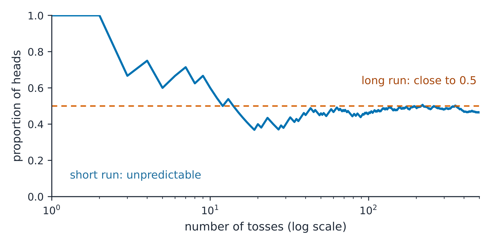
Something is random 随机 if individual outcomes 结果 are uncertain but a regular pattern emerges over many repetitions 重复. Short-run results look erratic; long-run relative frequencies 相对频率 settle down. This long-run stability is what makes probability useful. A streak or a pattern in a short run of data does not by itself show that the process is not random: random processes produce streaks quite often.
The law of large numbers 大数定律: as the number of trials grows, the relative frequency of an event gets closer and closer to its true probability. It says nothing about the short run: after five heads in a row, a fair coin is still $50\%$ likely to land heads next.
Explore
A probability from 0 to 1
Probability lives on a scale from 0 (impossible) to 1 (certain).
Vocabulary
Train
| English |
|---|
| random/ˈrændəm/ |
| outcomes/ˈaʊtkʌmz/ |
| repetitions |
| relative frequencies/ˈrelətɪv ˈfriːkwənsiz/ |
| law of large numbers/lɔː ɒv lɑːdʒ ˈnʌmbəz/ |
4.2
Estimating Probabilities Using Simulation
Syllabus
| Enduring Understanding | Learning Objective | Essential Knowledge |
|---|---|---|
UNC-2 | UNC-2.A |
|
Source: College Board AP Course and Exam Description
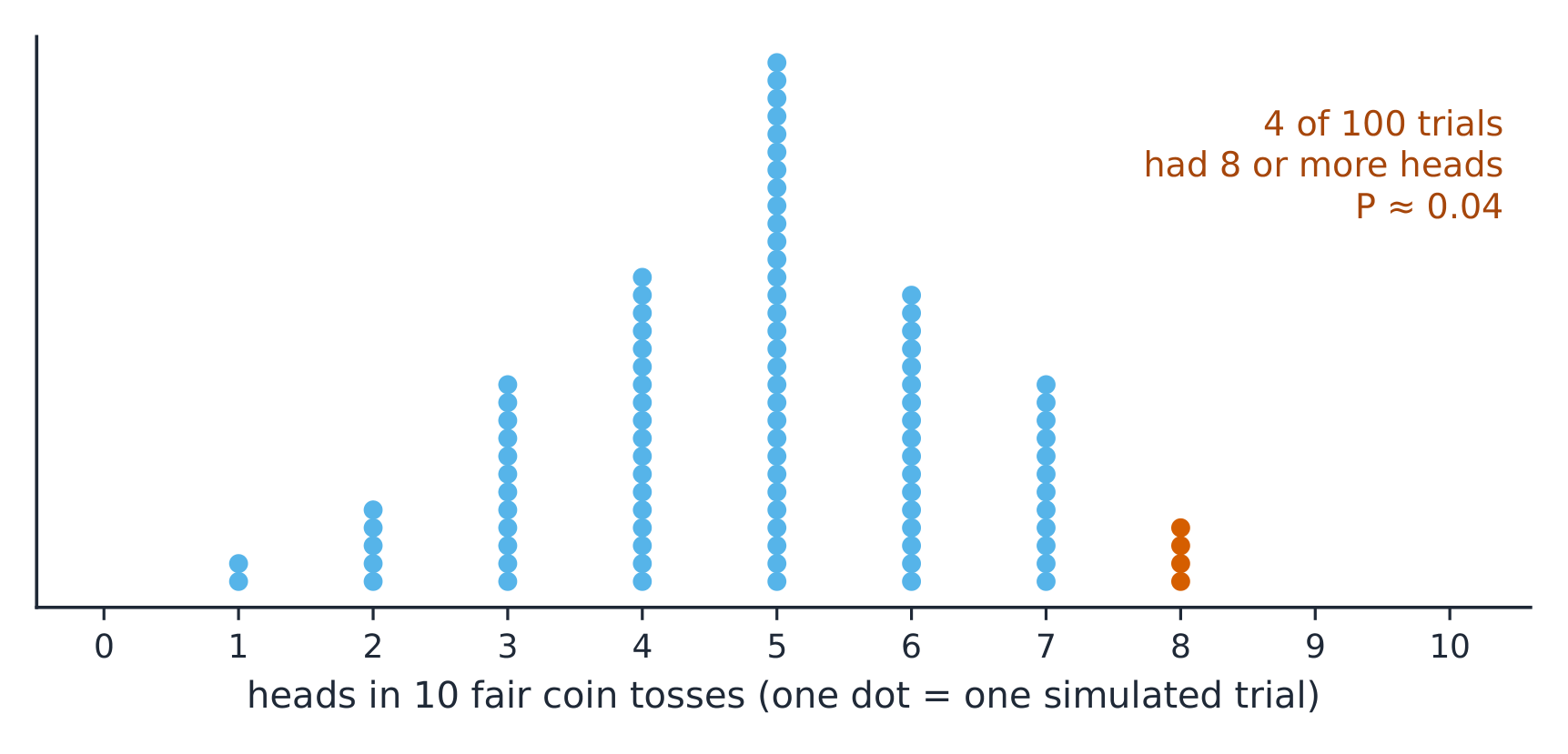
A simulation 模拟 imitates a chance process 随机过程 using random digits 随机数字 or technology. Steps: state the model, assign digits to outcomes, run many trials 试验, and record the proportion of trials meeting the condition. The resulting proportion estimates the probability – more trials give a better estimate.
Worked example (a complete simulation). Estimate the probability that choosing $3$ people at random from $6$ men and $3$ women gives $3$ women. Label the people $1$ to $9$, with $1$–$3$ the women. Use a random number generator to pick integers from $1$ to $9$, ignoring repeats, until $3$ different people are chosen; record whether all three are women. Repeat this many times (say $1000$). The proportion of trials with three women estimates the probability. A simulation description must say what the numbers stand for, how repeats are handled, what is recorded, and that the process is repeated many times.
Vocabulary
Train
| English |
|---|
| simulation/ˌsɪmjʊˈleɪʃn/ |
| chance process |
| random digits |
| trials |
4.3
Introduction to Probability

Syllabus
| Enduring Understanding | Learning Objective | Essential Knowledge |
|---|---|---|
VAR-4 | VAR-4.A |
|
VAR-4.B |
|
Source: College Board AP Course and Exam Description
The probability 概率 of an event 事件 is a number from $0$ to $1$ giving its long-run relative frequency. The sample space 样本空间 is the set of all outcomes. For an event $A$, the complement 补 rule: $P(A^c)=1-P(A)$. Probabilities of all outcomes sum to $1$. When all outcomes are equally likely,
$$P(A)=\frac{\text{number of outcomes in }A}{\text{total number of outcomes}}.$$
A probability is a long-run relative frequency. "$P(\text{rain})=0.3$" means that over many days like this one, it rains on about $30\%$ of them.
Worked example (is the claim believable?). For the manager's choice above, there are $\binom93=84$ equally likely groups of $3$, and only one of them is all three women: $P=\tfrac{1}{84}=0.012$. An outcome this unlikely under random selection gives reason to doubt that the choice was random. It does not prove unfairness: unlikely things do happen, about $1$ time in $84$.

Explore
Explore probability with dice
Probability is the long-run fraction of times an outcome happens. Roll the dice many times and watch the experimental proportions settle toward the theoretical values.
Vocabulary
Train
| English |
|---|
| probability/ˌprɒbəˈbɪlɪti/ |
| event/ɪˈvent/ |
| sample space/ˈsæmpl speɪs/ |
| complement/ˈkɒmplɪmənt/ |
4.4
Mutually Exclusive Events
Syllabus
| Enduring Understanding | Learning Objective | Essential Knowledge |
|---|---|---|
VAR-4 | VAR-4.C |
|
Source: College Board AP Course and Exam Description
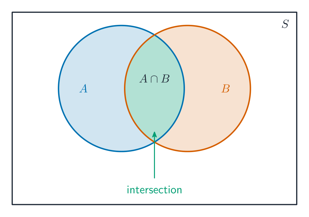
Two events are mutually exclusive 互斥 (disjoint 不相交) if they cannot both happen. Then the addition rule 加法法则 simplifies:
$$P(A\text{ or }B)=P(A)+P(B)\quad(\text{if mutually exclusive}).$$
In general, $P(A\text{ or }B)=P(A)+P(B)-P(A\text{ and }B)$ – subtract the overlap 重叠部分 so it is not counted twice.
Explore
Union of two events
The union is everything in A or B; subtract the overlap once.
Vocabulary
Train
| English |
|---|
| mutually exclusive/ˈmjuːtʃuːəli eksˈkluːsɪv/ |
| disjoint/dɪsˈdʒɔɪnt/ |
| addition rule/əˈdɪʃn ruːl/ |
| overlap/ˌəʊvəˈlæp/ |
4.5
Conditional Probability

Syllabus
| Enduring Understanding | Learning Objective | Essential Knowledge |
|---|---|---|
VAR-4 | VAR-4.D |
|
Source: College Board AP Course and Exam Description
The conditional probability 条件概率 of $A$ given $B$ is
$$P(A\mid B)=\frac{P(A\text{ and }B)}{P(B)}.$$
It is the chance of $A$ once you know $B$ happened. Two-way tables 双向表 make these easy: restrict to the row/column for $B$, then find $A$'s share.
Worked example: tree diagram. $2\%$ of people have a disease. A test is positive for $95\%$ of people who have it, and (a false positive 假阳性) for $10\%$ of people who do not. A person tests positive. What is the probability that they have the disease?
- Branch “disease, positive”: $0.02\times0.95=0.019$.
- Branch “no disease, positive”: $0.98\times0.10=0.098$.
- So $P(\text{positive})=0.019+0.098=0.117$.
$$P(\text{disease}\mid\text{positive})=\frac{P(\text{disease and positive})}{P(\text{positive})}=\frac{0.019}{0.117}\approx 0.162.$$
Only about $16\%$ of positive results come from people with the disease: so few people have it that the false positives outnumber the true ones. Do not confuse $P(\text{positive}\mid\text{disease})=0.95$ with $P(\text{disease}\mid\text{positive})$.
Explore
Update a probability on new information
Conditional probability $P(B\mid A)$ is the chance of $B$ once you know $A$ happened. Change the branch probabilities and watch how conditioning reshapes the outcome.
Vocabulary
Train
| English |
|---|
| conditional probability/kənˈdɪʃənl ˌprɒbəˈbɪlɪti/ |
| Two-way tables |
| false positive |
4.6
Independent Events and Unions of Events
Syllabus
| Enduring Understanding | Learning Objective | Essential Knowledge |
|---|---|---|
VAR-4 | VAR-4.E |
|
Source: College Board AP Course and Exam Description
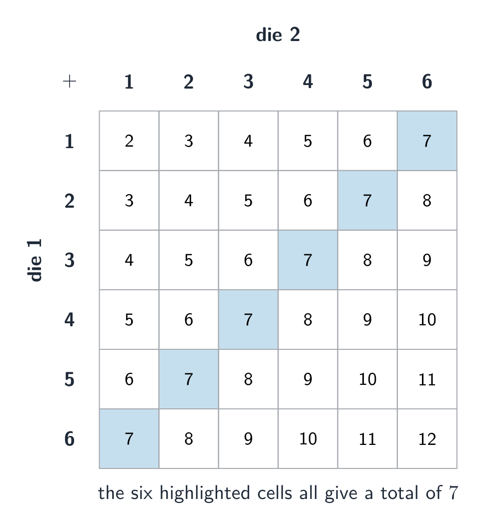
Events are independent 独立 if knowing one does not change the other's probability: $P(A\mid B)=P(A)$. Then the multiplication rule 乘法法则 simplifies:
$$P(A\text{ and }B)=P(A)\,P(B)\quad(\text{if independent}).$$
Independent is not the same as mutually exclusive – mutually exclusive events with nonzero probability are actually dependent 不独立 (if one happens, the other cannot).
"At least one": use the complement. A mall has three ATMs, each working at opening time with probability $0.9$, independently. The only way to have none working is all three failing:
$$P(\text{at least one works})=1-P(\text{none})=1-(0.1)^3=0.999.$$
Given that at least one works, the probability all three work is
$$P(\text{all}\mid\text{at least one})=\frac{P(\text{all and at least one})}{P(\text{at least one})}=\frac{0.9^3}{0.999}=\frac{0.729}{0.999}=0.730.$$
The "and" in the numerator is just $P(\text{all})$, because "all three work" is already inside "at least one works".
Explore
Combine events with a Venn diagram
For a union $P(A\cup B)=P(A)+P(B)-P(A\cap B)$ — you subtract the overlap so it isn't counted twice. Switch the operation to see each region light up.
Vocabulary
Train
| English |
|---|
| independent/ˌɪndɪˈpendənt/ |
| multiplication rule/ˌmʌltɪplɪˈkeɪʃn ruːl/ |
| dependent/dɪˈpendənt/ |
4.7
Random Variables and Probability Distributions

Syllabus
| Enduring Understanding | Learning Objective | Essential Knowledge |
|---|---|---|
VAR-5 | VAR-5.A |
|
VAR-5.B |
|
Source: College Board AP Course and Exam Description
A random variable 随机变量 assigns a number to each outcome of a chance process. A probability distribution 概率分布 lists each possible value with its probability (they sum to $1$). A distribution can be discrete 离散 (a table of values) or continuous 连续 (an area-under-a-curve model like the normal).
A cumulative probability distribution gives $P(X\le x)$ for each value, adding the probabilities up from the smallest value. Its last entry is always $1$. Two random variables are independent if knowing the value of one does not change the probability distribution of the other.
Explore
A discrete probability distribution
Each bar is P(x); the bars sum to 1.
Vocabulary
Train
| English |
|---|
| random variable/ˈrændəm ˈveərɪəbl/ |
| probability distribution/ˌprɒbəˈbɪlɪti ˌdɪstrɪˈbjuːʃn/ |
| discrete/dɪˈskriːt/ |
| continuous/kənˈtɪnjuːəs/ |
4.8
Mean and Standard Deviation of Random Variables
Syllabus
| Enduring Understanding | Learning Objective | Essential Knowledge |
|---|---|---|
VAR-5 | VAR-5.C |
|
VAR-5.D |
|
Source: College Board AP Course and Exam Description
The mean (expected value) 期望值 of a discrete random variable is the probability-weighted average 概率加权平均:
$$\mu_X=E(X)=\sum x_i\,P(x_i).$$
The standard deviation 标准差 $\sigma_X=\sqrt{\sum (x_i-\mu_X)^2\,P(x_i)}$ measures typical spread from the mean. The expected value is the long-run average outcome, not a value you expect on any single trial.
Worked example. A game pays $\$5$ with probability $0.2$ and costs you $\$1$ (a $-1$ outcome) with probability $0.8$. The expected value is
$$E(X)=5(0.2)+(-1)(0.8)=1-0.8=\$0.20,$$
so over many plays you gain about $20$ cents per play on average, even though no single play gives exactly that.
Worked example (the ATMs again). The number of working ATMs, $X$, has $E(X)=3(0.9)=2.7$. Interpretation in context: "Over many days, the mean number of ATMs working when the mall opens is about $2.7$." If we are told that at least one ATM works, the case $X=0$ is removed, so the expected value increases slightly: the remaining values are all $1$ or more.
Vocabulary
Train
| English |
|---|
| mean (expected value)/miːn/ |
| probability-weighted average |
| standard deviation/ˈstændəd ˌdiːvɪˈeɪʃn/ |
4.9
Combining Random Variables
Syllabus
| Enduring Understanding | Learning Objective | Essential Knowledge |
|---|---|---|
VAR-5 | VAR-5.E |
|
VAR-5.F |
|
Source: College Board AP Course and Exam Description
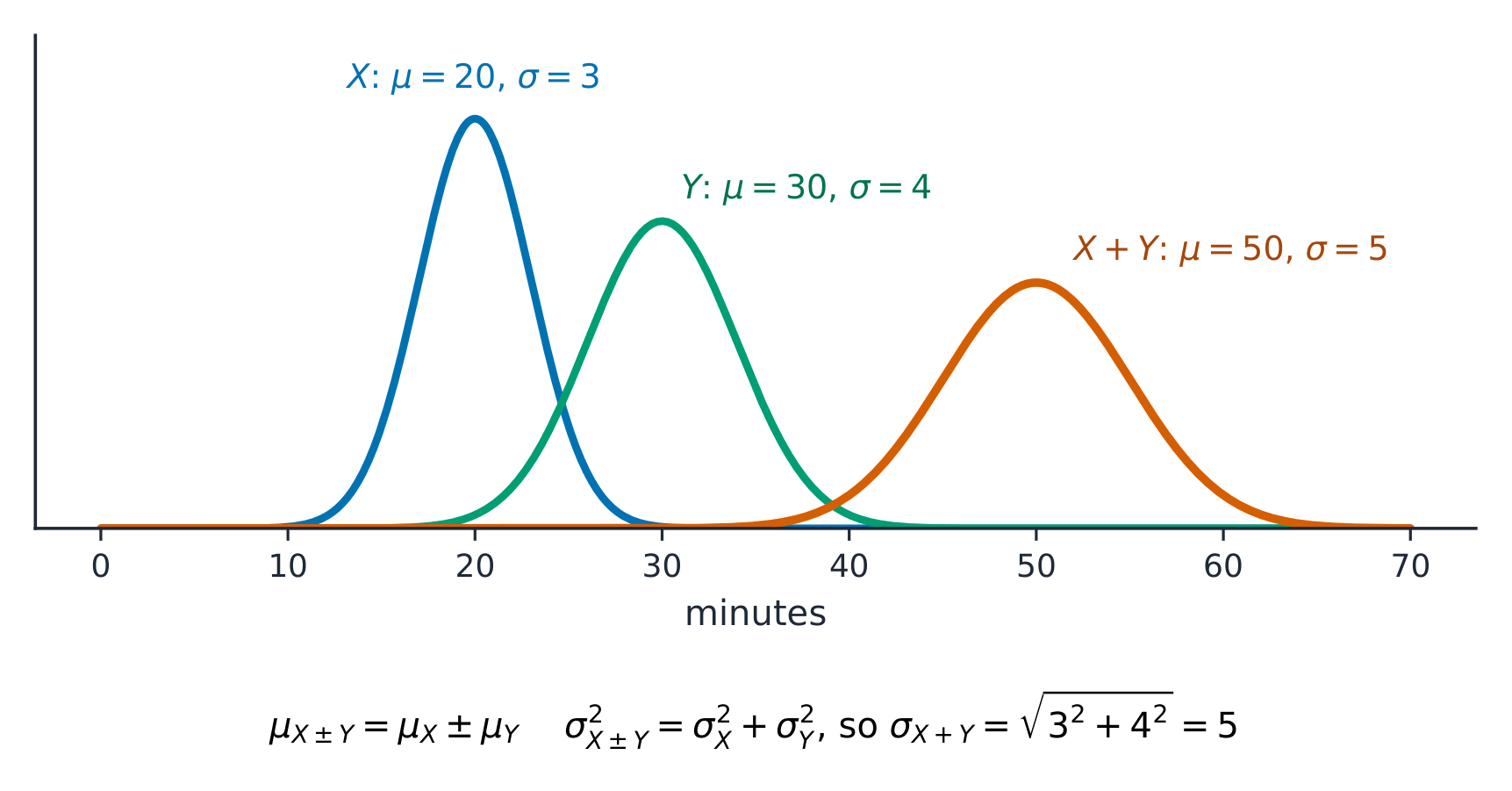
When you add or subtract random variables, means add 均值相加: $\mu_{X\pm Y}=\mu_X\pm\mu_Y$. If $X$ and $Y$ are independent, variances add 方差相加 (even when subtracting):
$$\sigma^2_{X\pm Y}=\sigma^2_X+\sigma^2_Y.$$
Take the square root for the standard deviation. Also, scaling: $\mu_{aX+b}=a\mu_X+b$ and $\sigma_{aX+b}=|a|\sigma_X$. A linear change $Y=a+bX$ does not change the shape of the distribution (for $b>0$): a right-skewed $X$ gives a right-skewed $Y$.
Worked example. Task A takes $X$ minutes with $\mu_X=20$, $\sigma_X=3$; task B takes $Y$ minutes with $\mu_Y=15$, $\sigma_Y=4$; the times are independent.
- Total time: $\mu_{X+Y}=20+15=35$ minutes, and $\sigma_{X+Y}=\sqrt{3^2+4^2}=\sqrt{25}=5$ minutes.
- Difference: $\mu_{X-Y}=20-15=5$ minutes, and $\sigma_{X-Y}=\sqrt{3^2+4^2}=5$ minutes as well.
Two common errors: adding the standard deviations ($3+4=7$), and subtracting them for a difference ($4-3=1$). Add the variances, then take the square root.
A third error: treating $3X$ like $X_1+X_2+X_3$. Tripling one value triples the spread, $\sigma_{3X}=3\sigma_X$; adding three independent values gives $\sigma=\sqrt{3}\,\sigma_X$, because the variances add.
Explore
A combined normal variable
A sum/difference of independent normals is itself normal.
Vocabulary
Train
| English |
|---|
| means add |
| variances add |
4.10
Introduction to the Binomial Distribution
Syllabus
| Enduring Understanding | Learning Objective | Essential Knowledge |
|---|---|---|
UNC-3 | UNC-3.A |
|
UNC-3.B |
|
Source: College Board AP Course and Exam Description
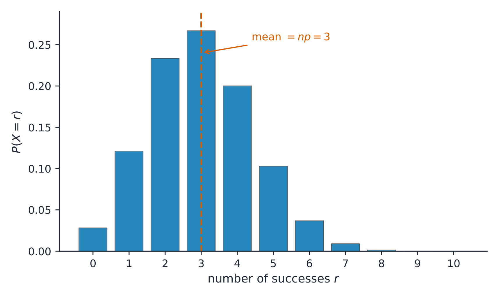
A binomial 二项 setting (BINS): a fixed number $n$ of Independent trials, each with two outcomes (success 成功/failure 失败) and the same success probability $p$. The random variable $X=$ number of successes. Its probability:
$$P(X=k)=\binom{n}{k}p^k(1-p)^{n-k}.$$
Explore
Shape a binomial distribution
A binomial distribution counts successes in $n$ independent trials each with probability $p$. Change $n$ and $p$ and watch the bars shift and spread.
Vocabulary
Train
| English |
|---|
| binomial/baɪˈnəʊmɪəl/ |
| success |
| failure |
4.11
Parameters for a Binomial Distribution
Syllabus
| Enduring Understanding | Learning Objective | Essential Knowledge |
|---|---|---|
UNC-3 | UNC-3.C |
|
UNC-3.D |
|
Source: College Board AP Course and Exam Description
For a binomial $X$ with $n$ trials and success probability $p$:
$$\mu_X=np,\qquad \sigma_X=\sqrt{np(1-p)}.$$
Use these for "how many successes do we expect, and how much do they vary" questions. Interpret them in context: "If we test many batches of $n$, the mean number of successes per batch is about $np$." A binomial distribution can also be built from the formula, or estimated by simulation.
Worked example. A player makes $70\%$ of free throws. In $n=10$ shots, the probability of exactly $8$ makes is
$$P(X=8)=\binom{10}{8}(0.7)^8(0.3)^2=45\times0.0576\times0.09\approx0.23,$$
and the expected number of makes is $\mu=np=10(0.7)=7$, with $\sigma=\sqrt{10(0.7)(0.3)}\approx1.45$.
Worked example: “at least”. For the same player ($n=10$, $p=0.7$), the probability of at least $8$ makes adds the top three values:
$$P(X\ge 8)=P(8)+P(9)+P(10)=0.2335+0.1211+0.0282=0.3828.$$
By the complement, the probability of at most $7$ makes is $P(X\le7)=1-0.3828=0.6172$.
Common mistakes. Writing $P(X\ge 8)=1-P(X\le 8)$: the complement of “at least $8$” is “at most $7$”, so $P(X\ge 8)=1-P(X\le 7)$. Using a binomial model when $n$ is not fixed, or when the trials are not independent (drawing without replacement from a small group).
4.12
The Geometric Distribution

Syllabus
| Enduring Understanding | Learning Objective | Essential Knowledge |
|---|---|---|
UNC-3 | UNC-3.E |
|
UNC-3.F |
| |
UNC-3.G |
|
Source: College Board AP Course and Exam Description
A geometric 几何 setting is the same as binomial but with no fixed $n$: you keep trying until the first success. The random variable $Y=$ the trial of the first success:
$$P(Y=k)=(1-p)^{k-1}\,p,\qquad \mu_Y=\frac{1}{p}.$$
So the expected number of trials until the first success is $1/p$.
Worked example. A player makes $30\%$ of shots, independently. The probability that the first make is on the third shot needs two misses, then a make:
$$P(Y=3)=(0.7)^2(0.3)=0.147.$$
The probability of a make within the first three shots uses the complement (three misses in a row): $P(Y\le 3)=1-0.7^3=0.657$. On average the first make comes on shot $\mu_Y=\tfrac{1}{0.3}\approx 3.33$. The standard deviation is $\sigma_Y=\dfrac{\sqrt{1-p}}{p}=\dfrac{\sqrt{0.7}}{0.3}=2.79$ shots.
Worked example (rocket igniters). A company claims a failure rate of $15\%$. The probability that the first $30$ igniters tested all work is $0.85^{30}=0.0076$. Getting $30$ successes in a row would be very unusual if the failure rate really were $15\%$, so it is reasonable to believe the failure rate is lower. Given those $30$ successes, the chance that the first failure is on test $31$ or $32$ is $0.15+0.85(0.15)=0.278$: past successes do not change the next trials, because they are independent.
Explore
Rolling until the first success
Keep rolling until the target appears — that's a geometric count.
Vocabulary
Train
| English |
|---|
| geometric/ˌdʒiːəʊˈmetrɪk/ |
4.12
Practice
Answer each before reading the answers below.
-
$P(A)=0.5$, $P(B)=0.4$ and $P(A\text{ and }B)=0.2$. Find $P(A\text{ or }B)$.
-
Are $A$ and $B$ in question 1 independent? Show why.
-
A basketball player makes $30\%$ of three-point shots, independently. In 10 shots, find the probability of exactly 2 makes.
-
A game costs $1 to play. You win $5 (and keep your $1) with probability $0.2$; otherwise you lose the $1. Find the expected gain per game.
-
A student says: "Mutually exclusive events are independent, because one has nothing to do with the other." Correct the student.
-
Each of $4$ independent smoke alarms works with probability $0.95$. Find the probability that at least one works.
-
In a large school, $40\%$ of students walk to school. If $8$ students are chosen at random, find the mean and standard deviation of the number who walk, and interpret the mean.
-
Machine A makes $60\%$ of a factory's bolts and $2\%$ of its bolts are faulty; machine B makes the rest, and $5\%$ of B's bolts are faulty. A bolt is faulty. Find the probability it came from machine A.
4.12
Answers
-
$P(A\text{ or }B)=0.5+0.4-0.2=0.7$.
-
Yes: $P(A)P(B)=0.5\times0.4=0.2=P(A\text{ and }B)$.
-
Binomial with $n=10$, $p=0.3$: $\binom{10}{2}(0.3)^2(0.7)^8=45(0.09)(0.0576)=0.233$.
-
$E=0.2(5)+0.8(-1)=0.20$: on average the player gains $0.20 per game.
-
If $A$ and $B$ are mutually exclusive and both have positive probability, then knowing $A$ happened tells you $B$ did not. So $P(B\mid A)=0\neq P(B)$: they are dependent, and as dependent as two events can be.
-
$1-0.05^4=1-0.00000625=0.99999$.
-
$\mu=8(0.4)=3.2$, $\sigma=\sqrt{8(0.4)(0.6)}=1.39$. In many random samples of $8$ students, the mean number who walk would be about $3.2$.
-
$P(\text{faulty})=0.6(0.02)+0.4(0.05)=0.012+0.020=0.032$, so $P(A\mid\text{faulty})=\dfrac{0.012}{0.032}=0.375$.
4.12
Exam tips
- A probability lies in $[0,1]$; use the complement ($1-P$) and add mutually exclusive events.
- For independent events multiply; for "and/or" use the general addition and conditional rules.
- Expected value = $\sum(\text{value}\times\text{probability})$.
- Recognise binomial (fixed $n$, two outcomes, constant $p$) and geometric settings.
- Draw a tree or table for multi-stage problems and multiply along branches.
- For "at least one", subtract "none" from $1$.
- When a result has a small probability under a claim, say it gives reason to doubt the claim, and quote the probability.
- Interpret an expected value as a long-run mean over many repetitions, in context.
Interactive lessons on this topic
Work through it step by step, with instant-check exercises.
- Random and Non-Random Patterns
- Estimating with Simulation
- Introduction to Probability
- Mutually Exclusive Events
- Conditional Probability
- Independent Events
- Random Variables
- Mean and SD of Random Variables
- Combining Random Variables
- The Binomial Distribution
- Binomial Parameters
- The Geometric Distribution