AP Statistics mencakup menjelajahi data, sampling dan desain eksperimen, probabilitas dan variabel acak, distribusi sampling, dan inferensi — interval kepercayaan dan uji signifikansi. Aljabar yang digunakan sangat sedikit; kesulitannya terletak pada menyatakan hal yang tepat mengenai ketidakpastian.
Setiap jawaban inferensi memiliki empat bagian: menamai prosedur, memeriksa syarat-syaratnya, menghitung, dan menyimpulkan dalam konteks dengan mengaitkannya ke hipotesis alternatif. Rubrik menilai keempat bagian tersebut, sehingga p-value yang benar saja tidak akan mendapatkan skor tinggi.
Bahasa dinilai. "Kami menolak H₀" bukan berarti "kami membuktikan H₁"; interval kepercayaan berkaitan dengan perilaku jangka panjang dari metode tersebut, bukan probabilitas bahwa interval tertentu memuat parameter. Perbedaan-perbedaan ini menentukan nilai yang diperoleh.
Catatan ini membahas semua sembilan unit dengan setiap prosedur inferensi diuraikan langkah demi langkah. FRQ (Free Response Questions) yang dirilis tersedia di perpustakaan. Statistik memberikan nilai untuk menyebutkan syarat-syaratnya dan menafsirkannya dalam konteks, sehingga setiap contoh jawaban yang dikerjakan selalu menyebutkan syarat-syaratnya sebelum melakukan pengujian.
Introducing Statistics: What Can We Learn from Data? · Memperkenalkan Statistik: Apa yang Bisa Kita Pelajari dari Data?
Syllabus · Silabus
English
Enduring Understanding (VAR-1): Given that variation may be random or not, conclusions are uncertain.
Learning Objective VAR-1.A: Identify questions to be answered, based on variation in one-variable data. [Skill 1.A]
VAR-1.A.1 Numbers may convey meaningful information, when placed in context.
Bahasa Indonesia
Pemahaman Abadi (VAR-1): Mengingat variasi bisa bersifat acak atau tidak, kesimpulan bersifat tidak pasti.
Tujuan Pembelajaran VAR-1.A: Identifikasi pertanyaan yang akan dijawab, berdasarkan variasi dalam data satu variabel. [Keterampilan 1.A]
VAR-1.A.1 Angka dapat menyampaikan informasi yang bermakna, ketika ditempatkan dalam konteks.
Source: College Board AP Course and Exam Description · Sumber: Deskripsi Kursus dan Ujian College Board AP
English
Statistics 统计学 is the science of learning from data 数据 – numbers or labels collected from the real world. Data vary, so we describe patterns and account for the variation 变异 rather than expecting every value to match. A statistical question anticipates an answer based on data that vary.
Two distinctions run through the whole course. A parameter 参数 is a numerical summary of a whole population; a statistic 统计量 is a numerical summary of a sample - we use the statistic to estimate the parameter we cannot measure directly. And descriptive statistics 描述统计 only summarise the data set in hand, while inferential statistics 推断统计 use a sample to make and test claims about the larger population.
Bahasa Indonesia
Statistik adalah ilmu mempelajari dari data – angka atau label yang dikumpulkan dari dunia nyata. Data bervariasi, jadi kita menggambarkan pola dan memperhitungkan variasi alih-alih mengharapkan setiap nilai sesuai. Pertanyaan statistik mengantisipasi jawaban berdasarkan data yang bervariasi.
Dua pembedaan melintasi seluruh kursus. Parameter adalah ringkasan numerik dari seluruh populasi; statistik adalah ringkasan numerik dari sampel - kita menggunakan statistik untuk memperkirakan parameter yang tidak dapat kita ukur secara langsung. Dan statistik deskriptif hanya merangkum himpunan data yang ada, sementara statistik inferensial menggunakan sampel untuk membuat dan menguji klaim tentang populasi yang lebih besar.
The Language of Variation: Variables · Bahasa Variasi: Variabel
Syllabus · Silabus
English
Enduring Understanding (VAR-1): Given that variation may be random or not, conclusions are uncertain.
Learning Objective VAR-1.B: Identify variables in a set of data. [Skill 2.A]
VAR-1.B.1 A variable is a characteristic that changes from one individual to another.
Learning Objective VAR-1.C: Classify types of variables. [Skill 2.A]
VAR-1.C.1 A categorical variable takes on values that are category names or group labels.
VAR-1.C.2 A quantitative variable is one that takes on numerical values for a measured or counted quantity.
Illustrative examples for VAR-1.C:
Categorical variables:
Dominant hand
Age group (young or old)
Highest degree earned
Quantitative variables:
Age of a structure
Height of a child
Concentration of a sample
Bahasa Indonesia
Pemahaman Abadi (VAR-1): Mengingat variasi bisa bersifat acak atau tidak, kesimpulan bersifat tidak pasti.
Tujuan Pembelajaran VAR-1.B: Identifikasi variabel dalam sekumpulan data. [Keterampilan 2.A]
VAR-1.B.1 Variabel adalah karakteristik yang berubah dari satu individu ke individu lain.
Tujuan Pembelajaran VAR-1.C: Klasifikasikan jenis variabel. [Keterampilan 2.A]
VAR-1.C.1 Variabel kategorikal mengambil nilai yang merupakan nama kategori atau label kelompok.
VAR-1.C.2 Variabel kuantitatif adalah variabel yang mengambil nilai numerik untuk kuantitas yang diukur atau dihitung.
Contoh ilustratif untuk VAR-1.C:
Variabel kategorikal:
Tangan dominan
Kelompok usia (muda atau tua)
Gelar tertinggi yang diraih
Variabel kuantitatif:
Umur suatu struktur
Tinggi seorang anak
Konsentrasi suatu sampel
Source: College Board AP Course and Exam Description · Sumber: Deskripsi Kursus dan Ujian College Board AP
English
A variable 变量 is a characteristic that can differ between individuals. Two kinds:
Categorical 分类 (qualitative): values are labels/groups (eye colour, brand).
Quantitative 定量: values are numbers you can do arithmetic on (height, age). Quantitative variables are discrete (countable) or continuous (measured).
Choosing the right graph and summary depends on which kind you have.
Bahasa Indonesia
Variabel adalah karakteristik yang dapat berbeda antar individu. Dua jenis:
Kategorikal (kualitatif): nilainya adalah label/kelompok (warna mata, merek).
Kuantitatif: nilainya adalah angka yang bisa Anda lakukan aritmatika padanya (tinggi badan, usia). Variabel kuantitatif bersifat diskrit (dapat dihitung) atau kontinu (diukur).
Memilih grafik dan ringkasan yang tepat bergantung pada jenis yang Anda miliki.
Explore · Jelajahi
Categorical or quantitative? · Kategorikal atau kuantitatif?
Every variable is either categorical (it labels each unit with a group) or quantitative (a measured number you can average). Which kind it is decides the graphs and summaries you are allowed to use. · Setiap variabel bersifat kategori (memberi label unit dengan kelompok) atau kuantitatif (angka terukur yang bisa dirata-ratakan). Jenisnya menentukan grafik dan ringkasan yang boleh Anda gunakan.
1.3
Representing a Categorical Variable with Tables · Mewakili Variabel Kategorikal dengan Tabel
Syllabus · Silabus
English
Enduring Understanding (UNC-1): Graphical representations and statistics allow us to identify and represent key features of data.
Learning Objective UNC-1.A: Represent categorical data using frequency or relative frequency tables. [Skill 2.B]
UNC-1.A.1 A frequency table gives the number of cases falling into each category. A relative frequency table gives the proportion of cases falling into each category.
Learning Objective UNC-1.B: Describe categorical data represented in frequency or relative tables. [Skill 2.A]
UNC-1.B.1 Percentages, relative frequencies, and rates all provide the same information as proportions.
UNC-1.B.2 Counts and relative frequencies of categorical data reveal information that can be used to justify claims about the data in context.
Bahasa Indonesia
Pemahaman Berkelanjutan (UNC-1): Representasi grafis dan statistik memungkinkan kita untuk mengidentifikasi dan merepresentasikan fitur utama dari data.
Tujuan Pembelajaran UNC-1.A: Mewakili data kategorikal menggunakan tabel frekuensi atau frekuensi relatif. [Keterampilan 2.B]
UNC-1.A.1 Tabel frekuensi memberikan jumlah kasus yang jatuh ke dalam setiap kategori. Tabel frekuensi relatif memberikan proporsi kasus yang jatuh ke dalam setiap kategori.
Tujuan Pembelajaran UNC-1.B: Mendeskripsikan data kategorikal yang direpresentasikan dalam tabel frekuensi atau tabel frekuensi relatif. [Keterampilan 2.A]
UNC-1.B.1 Persentase, frekuensi relatif, dan laju semuanya menyediakan informasi yang sama dengan proporsi.
UNC-1.B.2 Jumlah dan frekuensi relatif dari data kategorikal mengungkapkan informasi yang dapat digunakan untuk membenarkan klaim tentang data dalam konteksnya.
Source: College Board AP Course and Exam Description · Sumber: Deskripsi Kursus dan Ujian College Board AP
English
A frequency table 频数表 lists each category's count (frequency); a relative frequency 相对频率 table lists each category's proportion 比例 (count ÷ total). Relative frequencies let you compare groups of different sizes fairly.
Bahasa Indonesia
Tabel frekuensi mencantumkan jumlah (frekuensi) setiap kategori; tabel frekuensi relatif mencantumkan proporsi setiap kategori (jumlah ÷ total). Frekuensi relatif memungkinkan Anda membandingkan kelompok dengan ukuran berbeda secara adil.
1.4
Representing a Categorical Variable with Graphs · Mewakili Variabel Kategorikal dengan Grafik
Syllabus · Silabus
English
Enduring Understanding (UNC-1): Graphical representations and statistics allow us to identify and represent key features of data.
Learning Objective UNC-1.C: Represent categorical data graphically. [Skill 2.B]
UNC-1.C.1 Bar charts (or bar graphs) are used to display frequencies (counts) or relative frequencies (proportions) for categorical data.
UNC-1.C.2 The height or length of each bar in a bar graph corresponds to either the number or proportion of observations falling within each category.
UNC-1.C.3 There are many additional ways to represent frequencies (counts) or relative frequencies (proportions) for categorical data.
Learning Objective UNC-1.D: Describe categorical data represented graphically. [Skill 2.A]
UNC-1.D.1 Graphical representations of a categorical variable reveal information that can be used to justify claims about the data in context.
UNC-1.E.1 Frequency tables, bar graphs, or other representations can be used to compare two or more data sets in terms of the same categorical variable.
Bahasa Indonesia
Pemahaman Berkelanjutan (UNC-1): Representasi grafis dan statistik memungkinkan kita untuk mengidentifikasi dan merepresentasikan fitur utama dari data.
Tujuan Pembelajaran UNC-1.C: Mewakili data kategorikal secara grafis. [Keterampilan 2.B]
UNC-1.C.1 Diagram batang (atau grafik batang) digunakan untuk menampilkan frekuensi (jumlah) atau frekuensi relatif (proporsi) untuk data kategorikal.
UNC-1.C.2 Tinggi atau panjang setiap batang pada diagram batang sesuai dengan jumlah atau proporsi observasi yang jatuh ke dalam setiap kategori.
UNC-1.C.3 Ada banyak cara tambahan untuk merepresentasikan frekuensi (jumlah) atau frekuensi relatif (proporsi) untuk data kategorikal.
Tujuan Pembelajaran UNC-1.D: Mendeskripsikan data kategorikal yang direpresentasikan secara grafis. [Keterampilan 2.A]
UNC-1.D.1 Representasi grafis dari variabel kategorikal mengungkapkan informasi yang dapat digunakan untuk membenarkan klaim tentang data dalam konteksnya.
Tujuan Pembelajaran UNC-1.E: Membandingkan beberapa set data kategorikal. [Keterampilan 2.D]
UNC-1.E.1 Tabel frekuensi, diagram batang, atau representasi lain dapat digunakan untuk membandingkan dua set data atau lebih berdasarkan variabel kategorikal yang sama.
Source: College Board AP Course and Exam Description · Sumber: Deskripsi Kursus dan Ujian College Board AP
English
Bar charts 条形图 show the count or proportion of each category as separated bars; a pie chart shows each category's share of the whole. The bar heights (or slices) let you compare categories at a glance. Bars may be ordered by size or by a natural category order.
Bahasa Indonesia
Diagram batang menunjukkan jumlah atau proporsi setiap kategori sebagai batang terpisah; diagram lingkaran menunjukkan porsi setiap kategori dari keseluruhan. Tinggi batang (atau irisan) memungkinkan Anda membandingkan kategori sekilas. Batang dapat diurutkan berdasarkan ukuran atau urutan kategori alami.
Explore · Jelajahi
Show a categorical variable as a pie chart · Tampilkan variabel kategori sebagai diagram pie
A pie chart turns each category's share of the whole into a slice: a bigger share is a bigger slice, and every slice together makes 100%. It is a picture of a relative-frequency table. · A diagram pie mengubah porsi setiap kategori terhadap keseluruhan menjadi irisan: porsi lebih besar adalah irisan lebih besar, dan semua irisan bersama-sama membentuk 100%. Ini adalah gambar dari tabel frekuensi relatif.
1.5
Representing a Quantitative Variable with Graphs · Mewakili Variabel Kuantitatif dengan Grafik
Syllabus · Silabus
English
Enduring Understanding (UNC-1): Graphical representations and statistics allow us to identify and represent key features of data.
Learning Objective UNC-1.F: Classify types of quantitative variables. [Skill 2.A]
UNC-1.F.1 A discrete variable can take on a countable number of values. The number of values may be finite or countably infinite, as with the counting numbers.
UNC-1.F.2 A continuous variable can take on infinitely many values, but those values cannot be counted. No matter how small the interval between two values of a continuous variable, it is always possible to determine another value between them.
Illustrative examples for UNC-1.F:
A discrete variable:
Number of students in a class
A continuous variable:
Height of a child
Learning Objective UNC-1.G: Represent quantitative data graphically. [Skill 2.B]
UNC-1.G.1 In a histogram, the height of each bar shows the number or proportion of observations that fall within the interval corresponding to that bar. Altering the interval widths can change the appearance of the histogram.
UNC-1.G.2 In a stem and leaf plot, each data value is split into a "stem" (the first digit or digits) and a "leaf" (usually the last digit).
UNC-1.G.3 A dotplot represents each observation by a dot, with the position on the horizontal axis corresponding to the data value of that observation, with nearly identical values stacked on top of each other.
UNC-1.G.4 A cumulative graph represents the number or proportion of a data set less than or equal to a given number.
UNC-1.G.5 There are many additional ways to graphically represent distributions of quantitative data.
Bahasa Indonesia
Pemahaman Berkelanjutan (UNC-1): Representasi grafis dan statistik memungkinkan kita untuk mengidentifikasi dan merepresentasikan fitur utama dari data.
Tujuan Pembelajaran UNC-1.F: Mengklasifikasikan jenis variabel kuantitatif. [Keterampilan 2.A]
UNC-1.F.1 Variabel diskrit dapat mengambil sejumlah nilai yang dapat dihitung. Jumlah nilainya mungkin terbatas atau tak hingga yang dapat dihitung, seperti bilangan cacah.
UNC-1.F.2 Variabel kontinu dapat mengambil tak hingga banyak nilai, tetapi nilai-nilai tersebut tidak dapat dihitung. Sekecil apa pun interval antara dua nilai variabel kontinu, selalu mungkin untuk menentukan nilai lain di antaranya.
Contoh ilustratif untuk UNC-1.F:
Variabel diskrit:
Jumlah siswa dalam sebuah kelas
Variabel kontinu:
Tinggi seorang anak
Tujuan Pembelajaran UNC-1.G: Mewakili data kuantitatif secara grafis. [Keterampilan 2.B]
UNC-1.G.1 Dalam histogram, tinggi setiap batang menunjukkan jumlah atau proporsi observasi yang jatuh ke dalam interval yang sesuai dengan batang tersebut. Mengubah lebar interval dapat mengubah tampilan histogram.
UNC-1.G.2 Dalam diagram batang daun, setiap nilai data dibagi menjadi "batang" (digit pertama atau digit-digit awal) dan "daun" (biasanya digit terakhir).
UNC-1.G.3 Dotplot merepresentasikan setiap observasi dengan titik, dengan posisi pada sumbu horizontal yang sesuai dengan nilai data dari observasi tersebut, dengan nilai yang hampir identik ditumpuk satu sama lain.
UNC-1.G.4 Grafik kumulatif merepresentasikan jumlah atau proporsi dari himpunan data yang kurang dari atau sama dengan angka tertentu.
UNC-1.G.5 Ada banyak cara tambahan untuk merepresentasikan distribusi data kuantitatif secara grafis.
Source: College Board AP Course and Exam Description · Sumber: Deskripsi Kursus dan Ujian College Board AP
English
For numbers, use a dotplot 点图, stem-and-leaf plot 茎叶图, or histogram 直方图 (bars over value intervals called bins). These show the distribution 分布 – how the values spread out. A histogram's bin width changes the picture, so choose it to reveal the shape.
Bahasa Indonesia
Untuk angka, gunakan dotplot, stem-and-leaf plot, atau histogram (batang di atas interval nilai yang disebut bin). Ini menunjukkan distribusi – bagaimana nilai-nilai tersebar. Lebar bin histogram mengubah tampilan, jadi pilihlah untuk mengungkapkan bentuknya.
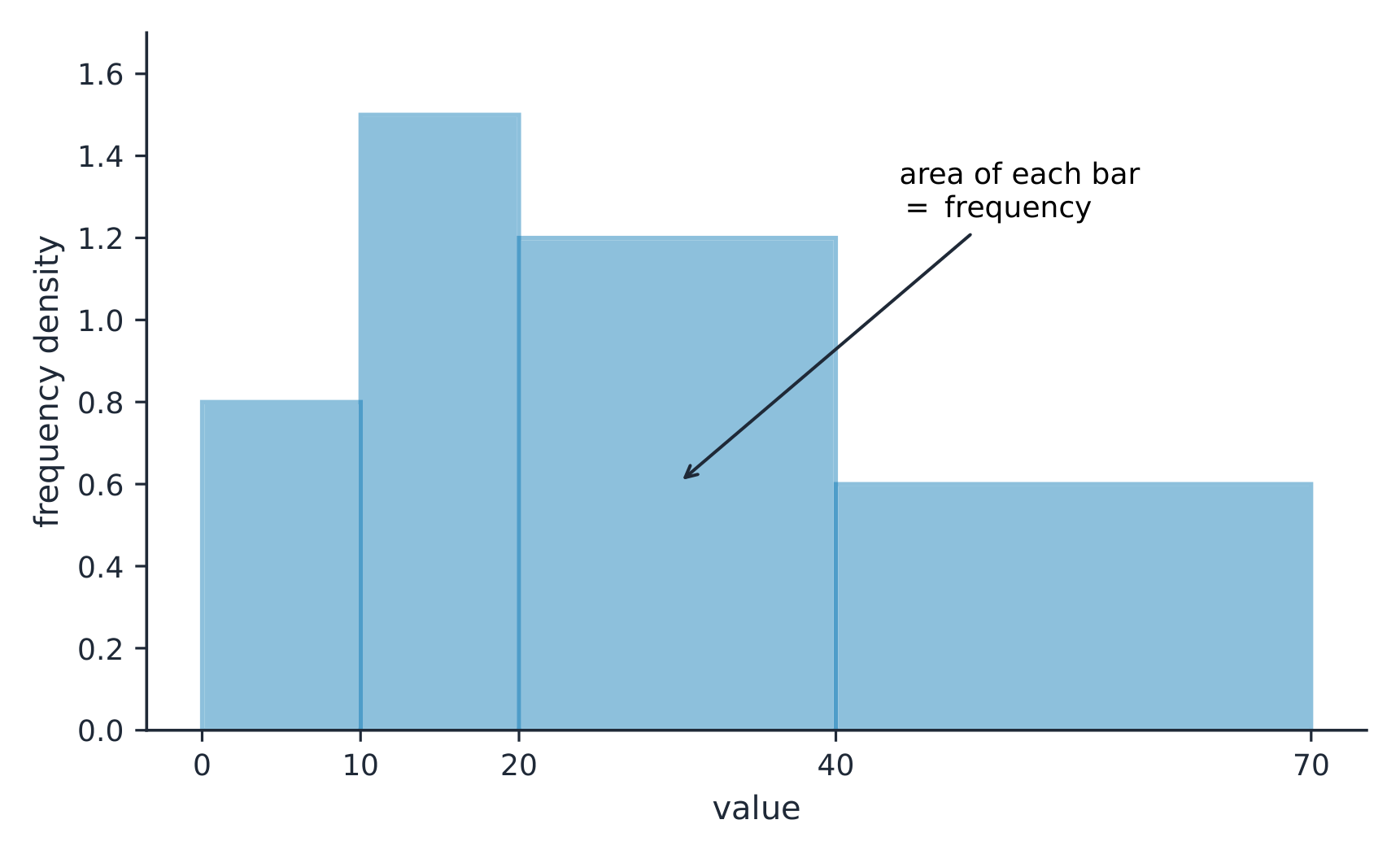
Pada histogram dengan lebar kelas tidak sama, luas batang adalah frekuensi
Explore · Jelajahi
Explore how bin width shapes a histogram · Jelajahi bagaimana lebar bin membentuk histogram
A histogram groups data into equal-width bins and draws a bar over each. Change the bins and notice how the same data can look jagged (too narrow) or smooth (too wide) — the shape is a choice. · A histogram mengelompokkan data ke dalam bin berlebar sama dan menggambar batang di atas masing-masing. Ubah bin-nya dan perhatikan bagaimana data yang sama bisa terlihat bergerigi (terlalu sempit) atau halus (terlalu lebar) — bentuknya adalah pilihan.
Describing the Distribution of a Quantitative Variable · Mendeskripsikan Distribusi Variabel Kuantitatif
Syllabus · Silabus
English
Enduring Understanding (UNC-1): Graphical representations and statistics allow us to identify and represent key features of data.
Learning Objective UNC-1.H: Describe the characteristics of quantitative data distributions. [Skill 2.A]
UNC-1.H.1 Descriptions of the distribution of quantitative data include shape, center, and variability (spread), as well as any unusual features such as outliers, gaps, clusters, or multiple peaks.
UNC-1.H.2 Outliers for one-variable data are data points that are unusually small or large relative to the rest of the data.
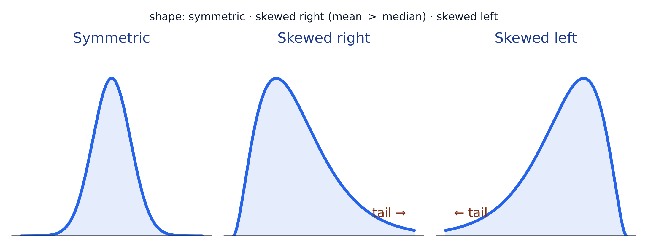
UNC-1.H.3 A distribution is skewed to the right (positive skew) if the right tail is longer than the left. A distribution is skewed to the left (negative skew) if the left tail is longer than the right. A distribution is symmetric if the left half is the mirror image of the right half.
UNC-1.H.4 Univariate graphs with one main peak are known as unimodal. Graphs with two prominent peaks are bimodal. A graph where each bar height is approximately the same (no prominent peaks) is approximately uniform.
UNC-1.H.5 A gap is a region of a distribution between two data values where there are no observed data.
UNC-1.H.6 Clusters are concentrations of data usually separated by gaps.
UNC-1.H.7 Descriptive statistics does not attribute properties of a data set to a larger population, but may provide the basis for conjectures for subsequent testing.
Bahasa Indonesia
Pemahaman Berkelanjutan (UNC-1): Representasi grafis dan statistik memungkinkan kita untuk mengidentifikasi dan merepresentasikan fitur utama dari data.
Tujuan Pembelajaran UNC-1.H: Mendeskripsikan karakteristik distribusi data kuantitatif. [Keterampilan 2.A]
UNC-1.H.1 Deskripsi distribusi data kuantitatif mencakup bentuk, pusat, dan variabilitas (sebaran), serta fitur-fitur tidak biasa seperti pencilan, celah, kluster, atau puncak ganda.
UNC-1.H.2 Pencilan untuk data satu variabel adalah titik data yang terlalu kecil atau terlalu besar dibandingkan dengan sisa data.
UNC-1.H.3 Distribusi miring ke kanan (skewness positif) jika ekor kanan lebih panjang daripada kiri. Distribusi miring ke kiri (skewness negatif) jika ekor kiri lebih panjang daripada kanan. Distribusi simetris jika setengah kiri adalah bayangan cermin dari setengah kanan.
UNC-1.H.4 Grafik univariat dengan satu puncak utama dikenal sebagai unimodal. Grafik dengan dua puncak menonjol adalah bimodal. Grafik di mana tinggi setiap batang kira-kira sama (tidak ada puncak menonjol) adalah mendekati seragam.
UNC-1.H.5 Celah adalah wilayah dari distribusi antara dua nilai data di mana tidak ada data yang teramati.
UNC-1.H.6 Kluster adalah konsentrasi data yang biasanya dipisahkan oleh celah.
UNC-1.H.7 Statistik deskriptif tidak atribut sifat-sifat dari himpunan data kepada populasi yang lebih besar, tetapi dapat menyediakan dasar untuk spekulasi pengujian lanjutan.
Source: College Board AP Course and Exam Description · Sumber: Deskripsi Kursus dan Ujian College Board AP
English
Describe four things (remember SOCS):
Shape 形状: symmetric, or skewed 偏斜 left/right (a long tail on that side), and how many peaks - one main peak is unimodal 单峰, two prominent peaks bimodal 双峰, and roughly equal bars uniform 均匀.
Outliers 离群值: unusual values far from the rest.
Center: a typical value (mean or median).
Spread: how much the values vary (range, IQR, standard deviation).
Always describe shape/center/spread in context, with units.
Bahasa Indonesia
Deskripsikan empat hal (ingat SOCS):
Bentuk: simetris, atau menceng ke kiri/kanan (ekor panjang di sisi itu), dan berapa banyak puncak - satu puncak utama adalah unimodal, dua puncak menonjol bimodal, dan batang yang kira-kira sama uniform.
Pencilan: nilai yang tidak biasa jauh dari yang lain.
Tengah: nilai tipikal (mean atau median).
Spread: seberapa besar nilai-nilai bervariasi (rentang, IQR, simpangan baku).
Selalu deskripsikan bentuk/pusat/sebaran dalam konteks, dengan satuan.
Bentuk distribusi: simetris, miring kanan (ekor kanan panjang), atau miring kiri
Summary Statistics for a Quantitative Variable · Ringkasan Statistik untuk Variabel Kuantitatif
Syllabus · Silabus
English
Enduring Understanding (UNC-1): Graphical representations and statistics allow us to identify and represent key features of data.
Learning Objective UNC-1.I: Calculate measures of center and position for quantitative data. [Skill 2.C]
UNC-1.I.1 A statistic is a numerical summary of sample data.
UNC-1.I.2 The mean is the sum of all the data values divided by the number of values. For a sample, the mean is denoted by $x$-bar: $\bar{x} = \dfrac{1}{n}\sum_{i=1}^{n} x_i$, where $x_i$ represents the $i^{\text{th}}$ data point in the sample and $n$ represents the number of data values in the sample.
UNC-1.I.3 The median of a data set is the middle value when data are ordered. When the number of data points is even, the median can take on any value between the two middle values. In AP Statistics, the most commonly used value for the median of a data set with an even number of values is the average of the two middle values.
UNC-1.I.4 The first quartile, Q1, is the median of the half of the ordered data set from the minimum to the position of the median. The third quartile, Q3, is the median of the half of the ordered data set from the position of the median to the maximum. Q1 and Q3 form the boundaries for the middle 50% of values in an ordered data set.
UNC-1.I.5 The $p^{\text{th}}$ percentile is interpreted as the value that has $p\%$ of the data less than or equal to it.
Learning Objective UNC-1.J: Calculate measures of variability for quantitative data. [Skill 2.C]
UNC-1.J.1 Three commonly used measures of variability (or spread) in a distribution are the range, interquartile range, and standard deviation.
UNC-1.J.2 The range is defined as the difference between the maximum data value and the minimum data value. The interquartile range (IQR) is defined as the difference between the third and first quartiles: $Q3 - Q1$. Both the range and the interquartile range are possible ways of measuring variability of the distribution of a quantitative variable.
UNC-1.J.3 Standard deviation is a way to measure variability of the distribution of a quantitative variable. For a sample, the standard deviation is denoted by $s$: $s_x = \sqrt{\dfrac{1}{n-1}\sum(x_i - \bar{x})^2}$. The square of the sample standard deviation, $s^2$, is called the sample variance.
UNC-1.J.4 Changing units of measurement affects the values of the calculated statistics.
Learning Objective UNC-1.K: Explain the selection of a particular measure of center and/or variability for describing a set of quantitative data. [Skill 4.B]
UNC-1.K.1 There are many methods for determining outliers. Two methods frequently used in this course are:
UNC-1.K.1.i An outlier is a value greater than $1.5 \times \text{IQR}$ above the third quartile or more than $1.5 \times \text{IQR}$ below the first quartile.
UNC-1.K.1.ii An outlier is a value located 2 or more standard deviations above, or below, the mean.
UNC-1.K.2 The mean, standard deviation, and range are considered nonresistant (or non-robust) because they are influenced by outliers. The median and IQR are considered resistant (or robust), because outliers do not greatly (if at all) affect their value.
Bahasa Indonesia
Pemahaman Berkelanjutan (UNC-1): Representasi grafis dan statistik memungkinkan kita untuk mengidentifikasi dan merepresentasikan fitur utama dari data.
Tujuan Pembelajaran UNC-1.I: Menghitung ukuran pusat dan posisi untuk data kuantitatif. [Keterampilan 2.C]
UNC-1.I.1 Statistik adalah ringkasan numerik dari data sampel.
UNC-1.I.2 Rata-rata adalah jumlah seluruh nilai data dibagi dengan banyak nilai. Untuk suatu sampel, rata-rata dilambangkan dengan $x$-bar: $\bar{x} = \dfrac{1}{n}\sum_{i=1}^{n} x_i$, di mana $x_i$ merepresentasikan titik data ke-$i^{\text{th}}$ dalam sampel dan $n$ merepresentasikan banyak nilai data dalam sampel.
UNC-1.I.3 Median dari suatu himpunan data adalah nilai tengah ketika data diurutkan. Ketika banyak titik data genap, median dapat mengambil nilai apa pun antara dua nilai tengah. Dalam Statistika AP, nilai yang paling umum digunakan untuk median dari himpunan data dengan banyak nilai genap adalah rata-rata dari dua nilai tengah tersebut.
UNC-1.I.4 Kuartil pertama, Q1, adalah median dari setengah himpunan data terurut mulai dari minimum hingga posisi median. Kuartil ketiga, Q3, adalah median dari setengah himpunan data terurut mulai dari posisi median hingga maksimum. Q1 dan Q3 membentuk batas untuk 50% nilai tengah dalam himpunan data terurut.
UNC-1.I.5 Persentil ke-$p^{\text{th}}$ ditafsirkan sebagai nilai yang memiliki $p\%$ bagian data kurang dari atau sama dengannya.
Tujuan Pembelajaran UNC-1.J: Hitung ukuran variabilitas untuk data kuantitatif. [Keterampilan 2.C]
UNC-1.J.1 Tiga ukuran variabilitas (atau sebaran) yang umum digunakan dalam distribusi adalah jangkauan, rentang interkuartil, dan simpangan baku.
UNC-1.J.2 Jangkauan didefinisikan sebagai selisih antara nilai data maksimum dan nilai data minimum. Rentang interkuartil (IQR) didefinisikan sebagai selisih antara kuartil ketiga dan kuartil pertama: $Q3 - Q1$. Baik jangkauan maupun rentang interkuartil merupakan cara yang mungkin untuk mengukur variabilitas distribusi variabel kuantitatif.
UNC-1.J.3 Simpangan baku adalah cara untuk mengukur variabilitas distribusi variabel kuantitatif. Untuk suatu sampel, simpangan baku dilambangkan dengan $s$: $s_x = \sqrt{\dfrac{1}{n-1}\sum(x_i - \bar{x})^2}$. Kuadrat dari simpangan baku sampel, $s^2$, disebut varians sampel.
UNC-1.J.4 Mengubah satuan pengukuran mempengaruhi nilai statistik yang dihitung.
Tujuan Pembelajaran UNC-1.K: Jelaskan pemilihan ukuran pusat dan/atau variabilitas tertentu untuk mendeskripsikan suatu set data kuantitatif. [Keterampilan 4.B]
UNC-1.K.1 Ada banyak metode untuk menentukan pencilan. Dua metode yang sering digunakan dalam kursus ini adalah:
UNC-1.K.1.i Pencilan adalah nilai lebih dari $1.5 \times \text{IQR}$ di atas kuartil ketiga atau lebih dari $1.5 \times \text{IQR}$ di bawah kuartil pertama.
UNC-1.K.1.ii Pencilan adalah nilai yang terletak 2 atau lebih simpangan baku di atas, atau di bawah, rata-rata.
UNC-1.K.2 Rata-rata, simpangan baku, dan jangkauan dianggap tidak resisten (atau tidak kuat) karena dipengaruhi oleh pencilan. Median dan IQR dianggap resisten (kuat), karena pencilan tidak secara signifikan (jika sama sekali) mempengaruhi nilainya.
Source: College Board AP Course and Exam Description · Sumber: Deskripsi Kursus dan Ujian College Board AP
English
Standard deviation: spread about the mean
Center: the mean 均值$\bar{x}=\dfrac{\sum x_i}{n}$ (average) and the median 中位数 (middle value). The median resists outliers; the mean is pulled toward a skew.
Spread: the range, the interquartile range 四分位距$\text{IQR}=Q_3-Q_1$ (middle 50%), and the standard deviation 标准差$s_x=\sqrt{\dfrac{\sum(x_i-\bar{x})^2}{n-1}}$ (typical distance from the mean; its square is the variance 方差).
The five-number summary 五数概括: min, $Q_1$, median, $Q_3$, max.
Use resistant measures (median, IQR) for skewed data; mean and standard deviation for roughly symmetric data.
The percentile 百分位数 of a value is the percent of the data at or below it – so the median is the 50th percentile and $Q_1$ the 25th. A cumulative relative frequency graph 累积相对频率图 makes percentiles easy to read: for each value it plots the proportion of the data at or below it, rising from 0 to 1. Go up from a value to the curve and across to its percentile, or reverse the steps to find the value at a given percentile (the same reading works from a cumulative-frequency table).
Worked example. For the data $4, 8, 6, 10, 7$: the mean is $\bar{x}=\dfrac{4+8+6+10+7}{5}=\dfrac{35}{5}=7$. Sorting to $4,6,7,8,10$, the median is the middle value, $7$. The mean and median agree here because the data are roughly symmetric.
Bahasa Indonesia
Simpangan baku: sebaran di sekitar rata-rata
Pusat:mean$\bar{x}=\dfrac{\sum x_i}{n}$ (rata-rata) dan median (nilai tengah). Median tahan terhadap pencilan; mean tertarik ke arah kemencengan.
Sebaran:rentang, rentang antar kuartil$\text{IQR}=Q_3-Q_1$ (50% tengah), dan simpangan baku$s_x=\sqrt{\dfrac{\sum(x_i-\bar{x})^2}{n-1}}$ (jarak tipikal dari rata-rata; kuadratnya adalah varians).
Ringkasan lima angka: min, $Q_1$, median, $Q_3$, max.
Gunakan ukuran tahan (median, IQR) untuk data yang menceng; mean dan simpangan baku untuk data yang hampir simetris.
Persentil dari suatu nilai adalah persentase data yang berada pada atau di bawahnya—sehingga median adalah persentil ke-50 dan $Q_1$ adalah persentil ke-25. Graf frekuensi relatif kumulatif memudahkan pembacaan persentil: untuk setiap nilai, graf memplot proporsi data pada atau di bawah nilai tersebut, naik dari 0 hingga 1. Naik dari sebuah nilai ke kurva lalu melintang ke persentilnya, atau sebaliknya untuk menemukan nilai pada persentil tertentu (pembacaan yang sama berlaku dari tabel frekuensi kumulatif).
Contoh terpecahkan. Untuk data $4, 8, 6, 10, 7$: mean adalah $\bar{x}=\dfrac{4+8+6+10+7}{5}=\dfrac{35}{5}=7$. Mengurutkan ke $4,6,7,8,10$, median adalah nilai tengah, $7$. Mean dan median sepakat di sini karena data hampir simetris.
cumulative relative frequency graph/ˈkjuːmjʊlətɪv ˈrelətɪv ˈfriːkwənsi ɡræf/
grafik frekuensi relatif kumulatif
1.8
Graphical Representations of Summary Statistics · Representasi Grafis dari Ringkasan Statistik
Syllabus · Silabus
English
Enduring Understanding (UNC-1): Graphical representations and statistics allow us to identify and represent key features of data.
Learning Objective UNC-1.L: Represent summary statistics for quantitative data graphically. [Skill 2.B]
UNC-1.L.1 Taken together, the minimum data value, the first quartile (Q1), the median, the third quartile (Q3), and the maximum data value make up the five-number summary.
UNC-1.L.2 A boxplot is a graphical representation of the five-number summary (minimum, first quartile, median, third quartile, maximum). The box represents the middle 50% of data, with a line at the median and the ends of the box corresponding to the quartiles. Lines ("whiskers") extend from the quartiles to the most extreme point that is not an outlier, and outliers are indicated by their own symbol beyond this.
Learning Objective UNC-1.M: Describe summary statistics of quantitative data represented graphically. [Skill 2.A]
UNC-1.M.1 Summary statistics of quantitative data, or of sets of quantitative data, can be used to justify claims about the data in context.
UNC-1.M.2 If a distribution is relatively symmetric, then the mean and median are relatively close to one another. If a distribution is skewed right, then the mean is usually to the right of the median. If the distribution is skewed left, then the mean is usually to the left of the median.
Bahasa Indonesia
Pemahaman Berkelanjutan (UNC-1): Representasi grafis dan statistik memungkinkan kita untuk mengidentifikasi dan merepresentasikan fitur utama dari data.
Tujuan Pembelajaran UNC-1.L: Representasikan statistik ringkasan untuk data kuantitatif secara grafis. [Keterampilan 2.B]
UNC-1.L.1 Secara bersama-sama, nilai data minimum, kuartil pertama (Q1), median, kuartil ketiga (Q3), dan nilai data maksimum membentuk lima angka ringkasan.
UNC-1.L.2 Boxplot adalah representasi grafis dari lima angka ringkasan (minimum, kuartil pertama, median, kuartil ketiga, maksimum). Kotak mewakili 50% data tengah, dengan garis pada median dan ujung kotak sesuai dengan kuartil. Garis ("bulu") membentang dari kuartil ke titik paling ekstrem yang bukan pencilan, dan pencilan ditandai dengan simbolnya sendiri di luar itu.
Tujuan Pembelajaran UNC-1.M: Deskripsikan statistik ringkasan dari data kuantitatif yang direpresentasikan secara grafis. [Keterampilan 2.A]
UNC-1.M.1 Statistik ringkasan dari data kuantitatif, atau dari set data kuantitatif, dapat digunakan untuk memvalidasi klaim tentang data dalam konteksnya.
UNC-1.M.2 Jika distribusi relatif simetris, maka rata-rata dan median relatif berdekatan satu sama lain. Jika distribusi miring kanan, maka rata-rata biasanya berada di sebelah kanan median. Jika distribusi miring kiri, maka rata-rata biasanya berada di sebelah kiri median.
Source: College Board AP Course and Exam Description · Sumber: Deskripsi Kursus dan Ujian College Board AP
English
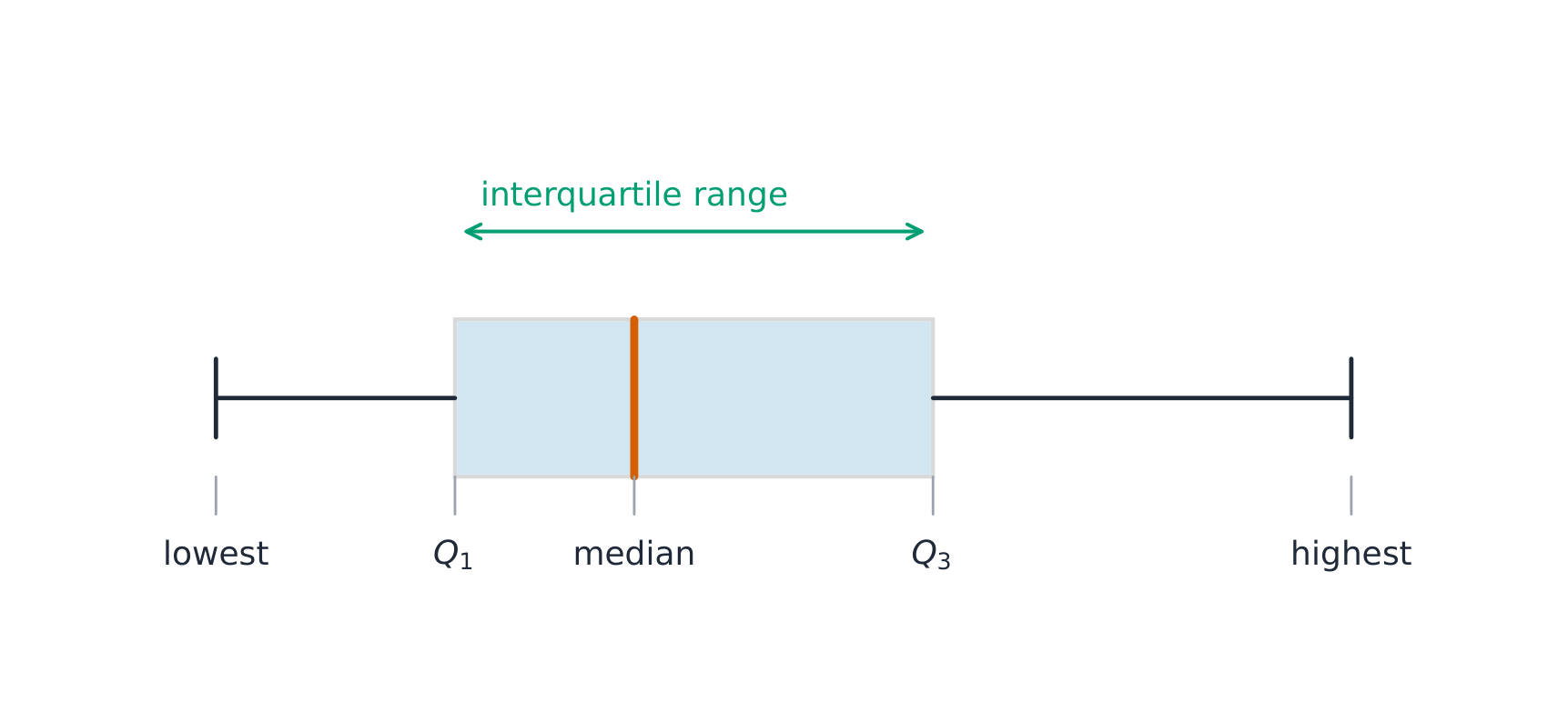
A boxplot 箱线图 draws the five-number summary: a box from $Q_1$ to $Q_3$ with the median inside, and whiskers to the most extreme non-outlier values. A point is an outlier if it lies more than $1.5\times\text{IQR}$ beyond a quartile – a rule you may be asked to apply. Boxplots are ideal for comparing several groups side by side.
Worked example. A dataset has $Q_1=20$ and $Q_3=32$, so $\text{IQR}=12$. The outlier fences are $Q_1-1.5(12)=2$ and $Q_3+1.5(12)=50$. Any value below $2$ or above $50$ is flagged as an outlier.
Bahasa Indonesia
Boxplot menggambar ringkasan lima angka: kotak dari $Q_1$ ke $Q_3$ dengan median di dalamnya, dan garis kumis menuju nilai ekstrem non-pencilan. Sebuah titik adalah pencilan jika terletak lebih dari $1.5\times\text{IQR}$ melampaui sebuah kuartil—aturan yang mungkin diminta untuk Anda terapkan. Boxplot sangat ideal untuk membandingkan beberapa kelompok berdampingan.
Contoh terpecahkan. Suatu dataset memiliki $Q_1=20$ dan $Q_3=32$, sehingga $\text{IQR}=12$. Pagar pencilan adalah $Q_1-1.5(12)=2$ dan $Q_3+1.5(12)=50$. Nilai apa pun di bawah $2$ atau di atas $50$ ditandai sebagai pencilan.
Diagram box-and-whisker menunjukkan kuartil dan rentangBoxplot menggambar ringkasan lima angka; kotak membentang sepanjang IQR
Explore · Jelajahi
Explore the five-number summary as a boxplot · Jelajahi ringkasan lima angka sebagai boxplot
Drag $Q_1$, the median, and $Q_3$ to see the box (its length is the IQR) and how the median's position inside the box reveals skew — a median close to $Q_1$ signals a right-skewed distribution. · Seret $Q_1$, median, dan $Q_3$ untuk melihat kotak (panjangnya adalah IQR) dan bagaimana posisi median di dalam kotak mengungkap kemencengan — median dekat dengan $Q_1$ mengindikasikan distribusi miring kanan.
Comparing Distributions of a Quantitative Variable · Membandingkan Distribusi Variabel Kuantitatif
Syllabus · Silabus
English
Enduring Understanding (UNC-1): Graphical representations and statistics allow us to identify and represent key features of data.
Learning Objective UNC-1.N: Compare graphical representations for multiple sets of quantitative data. [Skill 2.D]
UNC-1.N.1 Any of the graphical representations, e.g., histograms, side-by-side boxplots, etc., can be used to compare two or more independent samples on center, variability, clusters, gaps, outliers, and other features.
Learning Objective UNC-1.O: Compare summary statistics for multiple sets of quantitative data. [Skill 2.D]
UNC-1.O.1 Any of the numerical summaries (e.g., mean, standard deviation, relative frequency, etc.) can be used to compare two or more independent samples.
Bahasa Indonesia
Pemahaman Berkelanjutan (UNC-1): Representasi grafis dan statistik memungkinkan kita untuk mengidentifikasi dan merepresentasikan fitur utama dari data.
Tujuan Pembelajaran UNC-1.N: Bandingkan representasi grafis untuk beberapa set data kuantitatif. [Keterampilan 2.D]
UNC-1.N.1 Salah satu representasi grafis, mis., histogram, boxplot berdampingan, dll., dapat digunakan untuk membandingkan dua atau lebih sampel independen pada pusat, variabilitas, kluster, celah, pencilan, dan fitur lainnya.
Tujuan Pembelajaran UNC-1.O: Bandingkan statistik ringkasan untuk beberapa set data kuantitatif. [Keterampilan 2.D]
UNC-1.O.1 Salah satu ringkasan numerik (mis., rata-rata, simpangan baku, frekuensi relatif, dll.) dapat digunakan untuk membandingkan dua atau lebih sampel independen.
Source: College Board AP Course and Exam Description · Sumber: Deskripsi Kursus dan Ujian College Board AP
English
To compare two or more groups, compare shape, center, and spread, and mention outliers – always with comparative words ("Group A has a higher median than Group B") and in context. Do not just describe each group separately; make the comparison explicit.
Bahasa Indonesia
Untuk membandingkan dua atau lebih kelompok, bandingkan bentuk, pusat, dan sebaran, dan sebutkan pencilan—selalu dengan kata-kata perbandingan ("Kelompok A memiliki median yang lebih tinggi daripada Kelompok B") dan dalam konteks. Jangan hanya mendeskripsikan setiap kelompok secara terpisah; buat perbandingan secara eksplisit.
Explore · Jelajahi
Compare distributions with box plots · Bandingkan distribusi dengan box plot
A box plot draws the five-number summary. Placing two box plots on the same scale compares their centre (median), spread (IQR = box width) and skew at a glance — the fair way to compare groups. · A box plot menggambar ringkasan lima angka. Menempatkan dua box plot pada skala yang sama membandingkan pusat (median), sebaran (IQR = lebar kotak) dan kemencengan sekilas — cara adil untuk membandingkan kelompok.
1.10
The Normal Distribution · Distribusi Normal
Syllabus · Silabus
English
Enduring Understanding (VAR-2): The normal distribution can be used to represent some population distributions.
Learning Objective VAR-2.A: Compare a data distribution to the normal distribution model. [Skill 2.D]
VAR-2.A.1 A parameter is a numerical summary of a population.
VAR-2.A.2 Some sets of data may be described as approximately normally distributed. A normal curve is mound-shaped and symmetric. The parameters of a normal distribution are the population mean, $\mu$, and the population standard deviation, $\sigma$.
VAR-2.A.3 For a normal distribution, approximately 68% of the observations are within 1 standard deviation of the mean, approximately 95% of observations are within 2 standard deviations of the mean, and approximately 99.7% of observations are within 3 standard deviations of the mean. This is called the empirical rule.
VAR-2.A.4 Many variables can be modeled by a normal distribution.
Illustrative examples for VAR-2.A:
Variables that can be modeled by a normal distribution:
Body temperature
Weight of a loaf of bread
Learning Objective VAR-2.B: Determine proportions and percentiles from a normal distribution. [Skill 3.A]
VAR-2.B.1 A standardized score for a particular data value is calculated as (data value − mean)/(standard deviation), and measures the number of standard deviations a data value falls above or below the mean.
VAR-2.B.2 One example of a standardized score is a $z$-score, which is calculated as $z\text{-score} = \left(\dfrac{x_i - \mu}{\sigma}\right)$. A $z$-score measures how many standard deviations a data value is from the mean.
VAR-2.B.3 Technology, such as a calculator, a standard normal table, or computer-generated output, can be used to find the proportion of data values located on a given interval of a normally distributed random variable.
VAR-2.B.4 Given the area of a region under the graph of the normal distribution curve, it is possible to use technology, such as a calculator, a standard normal table, or computer-generated output, to estimate parameters for some populations.
Learning Objective VAR-2.C: Compare measures of relative position in data sets. [Skill 2.D]
VAR-2.C.1 Percentiles and $z$-scores may be used to compare relative positions of points within a data set or between data sets.
Bahasa Indonesia
Pemahaman Abadi (VAR-2): Distribusi normal dapat digunakan untuk merepresentasikan beberapa distribusi populasi.
Tujuan Pembelajaran VAR-2.A: Bandingkan distribusi data dengan model distribusi normal. [Keterampilan 2.D]
VAR-2.A.1 Parameter adalah ringkasan numerik dari suatu populasi.
VAR-2.A.2 Beberapa kumpulan data dapat digambarkan sebagai terdistribusi secara normal. Kurva normal berbentuk seperti gundukan dan simetris. Parameter dari distribusi normal adalah rata-rata populasi, $\mu$, dan simpangan baku populasi, $\sigma$.
VAR-2.A.3 Untuk distribusi normal, sekitar 68% observasi berada dalam 1 simpangan baku dari rata-rata, sekitar 95% observasi berada dalam 2 simpangan baku dari rata-rata, dan sekitar 99.7% observasi berada dalam 3 simpangan baku dari rata-rata. Ini disebut aturan empiris.
VAR-2.A.4 Banyak variabel dapat dimodelkan oleh distribusi normal.
Contoh ilustratif untuk VAR-2.A:
Variabel yang dapat dimodelkan oleh distribusi normal:
Suhu tubuh
Berat sepotong roti
Tujuan Pembelajaran VAR-2.B: Tentukan proporsi dan persentil dari distribusi normal. [Keterampilan 3.A]
VAR-2.B.1 Skor standar untuk nilai data tertentu dihitung sebagai (nilai data − rata-rata)/(simpangan baku), dan mengukur berapa banyak simpangan baku nilai data jatuh di atas atau di bawah rata-rata.
VAR-2.B.2 Salah satu contoh skor standar adalah skor $z$, yang dihitung sebagai $z\text{-score} = \left(\dfrac{x_i - \mu}{\sigma}\right)$. Skor $z$ mengukur berapa banyak simpangan baku nilai data dari rata-rata.
VAR-2.B.3 Teknologi, seperti kalkulator, tabel normal standar, atau output yang dihasilkan komputer, dapat digunakan untuk menemukan proporsi nilai data yang terletak pada interval tertentu dari variabel acak yang terdistribusi normal.
VAR-2.B.4 Diberikan luas daerah di bawah kurva distribusi normal, memungkinkan penggunaan teknologi, seperti kalkulator, tabel normal standar, atau output yang dihasilkan komputer, untuk memperkirakan parameter untuk beberapa populasi.
Tujuan Pembelajaran VAR-2.C: Bandingkan ukuran posisi relatif dalam kumpulan data. [Keterampilan 2.D]
VAR-2.C.1 Persentil dan skor $z$ dapat digunakan untuk membandingkan posisi relatif titik-titik dalam kumpulan data atau antar kumpulan data.
Source: College Board AP Course and Exam Description · Sumber: Deskripsi Kursus dan Ujian College Board AP
English
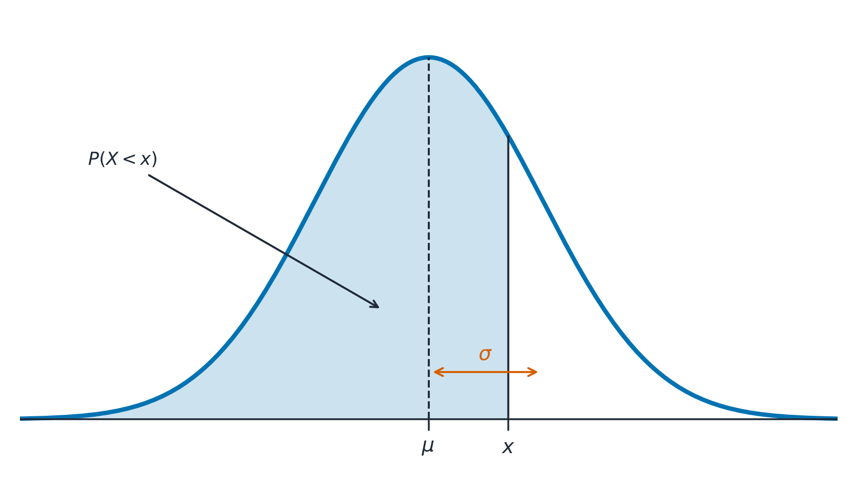
A normal distribution 正态分布 is a symmetric, bell-shaped model described by its mean $\mu$ and standard deviation $\sigma$. The empirical rule 经验法则 (68–95–99.7): about 68% of values lie within $1\sigma$ of the mean, 95% within $2\sigma$, and 99.7% within $3\sigma$.
A $z$-score 标准分数 measures how many standard deviations a value is from the mean:
$$z=\frac{x-\mu}{\sigma}.$$
Convert to a $z$-score, then use the normal table or technology to find the proportion (area) below, above, or between values – and reverse the process to find a value from a given percentile.
Worked example. Test scores are normal with $\mu=500$ and $\sigma=100$. A score of $700$ has $z=\dfrac{700-500}{100}=2$. By the empirical rule, $95\%$ of scores lie within $2\sigma$, so $2.5\%$ lie above $700$ – meaning a $700$ is at about the $97.5$th percentile.
Bahasa Indonesia
Distribusi normal adalah model simetris berbentuk lonceng yang dijelaskan oleh rata-rata $\mu$ dan simpangan baku $\sigma$. Aturan empiris (68–95–99.7): sekitar 68% nilai berada dalam $1\sigma$ dari rata-rata, 95% dalam $2\sigma$, dan 99.7% dalam $3\sigma$.
Kurva normal: probabilitas adalah luas di bawahnya, berpusat pada mean
Sebuah $z$-score mengukur berapa banyak simpangan baku suatu nilai berada dari mean:
$$z=\frac{x-\mu}{\sigma}.$$
Konversikan ke skor $z$, kemudian gunakan tabel normal atau teknologi untuk menemukan proporsi (luas area) di bawah, di atas, atau antara nilai—dan balik prosesnya untuk menemukan nilai dari persentil tertentu.
Contoh terpecahkan. Skor ujian berdistribusi normal dengan $\mu=500$ dan $\sigma=100$. Skor $700$ memiliki $z=\dfrac{700-500}{100}=2$. Berdasarkan aturan empiris, $95\%$ skor berada dalam $2\sigma$, sehingga $2.5\%$ berada di atas $700$—yang berarti skor $700$ berada di sekitar persentil ke-$97.5$.
Kurva normal dan aturan empiris 68-95-99.7
Explore · Jelajahi
Explore area under the normal curve · Jelajahi area di bawah kurva normal
The proportion of data below a value equals the area under the curve to its left. Shade a tail or a central band to see the 68–95–99.7 empirical rule and read a $z$-score as an area. · Proporsi data di bawah suatu nilai sama dengan area di bawah kurva ke kiri nilai tersebut. arsir ekor atau pita sentral untuk melihat aturan empiris 68–95–99.7 dan baca skor $z$ sebagai area.
Are Two Variables Related? · Apakah Dua Variabel Berkaitan?
Syllabus · Silabus
English
Enduring Understanding (VAR-1): Given that variation may be random or not, conclusions are uncertain.
Learning Objective VAR-1.D: Identify questions to be answered about possible relationships in data. [Skill 1.A]
VAR-1.D.1 Apparent patterns and associations in data may be random or not.
Bahasa Indonesia
Pemahaman Abadi (VAR-1): Mengingat variasi bisa bersifat acak atau tidak, kesimpulan bersifat tidak pasti.
Tujuan Pembelajaran VAR-1.D: Identifikasi pertanyaan yang akan dijawab mengenai kemungkinan hubungan dalam data. [Keterampilan 1.A]
VAR-1.D.1 Pola dan asosiasi yang tampak dalam data bisa bersifat acak atau tidak.
Source: College Board AP Course and Exam Description · Sumber: Deskripsi Kursus dan Ujian College Board AP
English
Two-variable data let us ask whether two characteristics are associated 关联 – whether knowing one tells you something about the other. An explanatory variable 解释变量 (the "input") may help predict a response variable 响应变量 (the "output"). Association is not the same as causation.
Bahasa Indonesia
Data dua variabel memungkinkan kita bertanya apakah dua karakteristik terkait—apakah mengetahui satu memberi informasi tentang yang lain. Variabel penjelas ("input") dapat membantu memprediksi variabel respons ("output"). Asosiasi bukan berarti sebab-akibat.
2.2
Two Categorical Variables · Dua Variabel Kategorikal
Syllabus · Silabus
English
Enduring Understanding (UNC-1): Graphical representations and statistics allow us to identify and represent key features of data.
Learning Objective UNC-1.P: Compare numerical and graphical representations for two categorical variables. [Skill 2.D]
UNC-1.P.1 Side-by-side bar graphs, segmented bar graphs, and mosaic plots are examples of bar graphs for one categorical variable, broken down by categories of another categorical variable.
UNC-1.P.2 Graphical representations of two categorical variables can be used to compare distributions and/or determine if variables are associated.
UNC-1.P.3 A two-way table, also called a contingency table, is used to summarize two categorical variables. The entries in the cells can be frequency counts or relative frequencies.
UNC-1.P.4 A joint relative frequency is a cell frequency divided by the total for the entire table.
Bahasa Indonesia
Pemahaman Berkelanjutan (UNC-1): Representasi grafis dan statistik memungkinkan kita untuk mengidentifikasi dan merepresentasikan fitur utama dari data.
Tujuan Pembelajaran UNC-1.P: Bandingkan representasi numerik dan grafis untuk dua variabel kategorikal. [Keterampilan 2.D]
UNC-1.P.1 Diagram batang berdampingan, diagram batang segmentasi, dan plot mozaik adalah contoh diagram batang untuk satu variabel kategorikal, yang diuraikan berdasarkan kategori dari variabel kategorikal lainnya.
UNC-1.P.2 Representasi grafis dari dua variabel kategorikal dapat digunakan untuk membandingkan distribusi dan/atau menentukan apakah variabel saling berasosiasi.
UNC-1.P.3 Tabel dua arah, juga disebut tabel kontingensi, digunakan untuk meringkas dua variabel kategorikal. Entri dalam sel dapat berupa jumlah frekuensi atau frekuensi relatif.
UNC-1.P.4 Frekuensi relatif gabungan adalah frekuensi sel dibagi dengan total keseluruhan tabel.
Source: College Board AP Course and Exam Description · Sumber: Deskripsi Kursus dan Ujian College Board AP
English
A two-way table 双向表 (contingency table) counts individuals by two categorical variables at once. A marginal distribution 边缘分布 is a row or column total written as a fraction of the grand total (the totals themselves are just counts). Comparing the inside cells shows whether the variables are related.
Bahasa Indonesia
Tabel dua arah (tabel kontingensi) menghitung jumlah individu berdasarkan dua variabel kategorikal sekaligus. Distribusi marginal adalah total baris atau kolom yang ditulis sebagai pecahan dari total keseluruhan (total itu sendiri hanyalah hitungan). Membandingkan sel-sel di bagian dalam menunjukkan apakah variabel tersebut terkait.
2.3
Comparing Groups with Conditional Distributions · Membandingkan Kelompok dengan Distribusi Bersyarat
Syllabus · Silabus
English
Enduring Understanding (UNC-1): Graphical representations and statistics allow us to identify and represent key features of data.
Learning Objective UNC-1.Q: Calculate statistics for two categorical variables. [Skill 2.C]
UNC-1.Q.1 The marginal relative frequencies are the row and column totals in a two-way table divided by the total for the entire table.
UNC-1.Q.2 A conditional relative frequency is a relative frequency for a specific part of the contingency table (e.g., cell frequencies in a row divided by the total for that row).
Learning Objective UNC-1.R: Compare statistics for two categorical variables. [Skill 2.D]
UNC-1.R.1 Summary statistics for two categorical variables can be used to compare distributions and/or determine if variables are associated.
Bahasa Indonesia
Pemahaman Berkelanjutan (UNC-1): Representasi grafis dan statistik memungkinkan kita untuk mengidentifikasi dan merepresentasikan fitur utama dari data.
Tujuan Pembelajaran UNC-1.Q: Hitung statistik untuk dua variabel kategorikal. [Keterampilan 2.C]
UNC-1.Q.1 Frekuensi relatif marginal adalah total baris dan kolom dalam tabel dua arah yang dibagi dengan total keseluruhan tabel.
UNC-1.Q.2 Frekuensi bersyarat adalah frekuensi relatif untuk bagian spesifik dari tabel kontingensi (misalnya, frekuensi sel dalam sebuah baris dibagi dengan total untuk baris tersebut).
Tujuan Pembelajaran UNC-1.R: Bandingkan statistik untuk dua variabel kategorikal. [Keterampilan 2.D]
UNC-1.R.1 Statistik ringkasan untuk dua variabel kategorikal dapat digunakan untuk membandingkan distribusi dan/atau menentukan apakah variabel-variabel tersebut相关联.
Source: College Board AP Course and Exam Description · Sumber: Deskripsi Kursus dan Ujian College Board AP
English
A conditional distribution 条件分布 is the distribution of one variable within a fixed category of the other (found by dividing each cell by its row or column total). If the conditional distributions differ across groups, the two variables are associated; if they are the same, there is no association. Segmented bar charts 分段条形图 or mosaic plots display them.
Bahasa Indonesia
Sebuah distribusi bersyarat adalah distribusi satu variabel di dalam kategori tetap dari variabel lainnya (ditemukan dengan membagi setiap sel dengan total baris atau kolomnya). Jika distribusi bersyarat berbeda di seluruh kelompok, kedua variabel tersebut terkait; jika sama, tidak ada asosiasi. Graf batang segmen atau plot mozaik menampilkan mereka.
2.4
Scatterplots for Two Quantitative Variables · Diagram Sebar untuk Dua Variabel Kuantitatif
Syllabus · Silabus
English
Enduring Understanding (UNC-1): Graphical representations and statistics allow us to identify and represent key features of data.
Learning Objective UNC-1.S: Represent bivariate quantitative data using scatterplots. [Skill 2.B]
UNC-1.S.1 A bivariate quantitative data set consists of observations of two different quantitative variables made on individuals in a sample or population.
UNC-1.S.2 A scatterplot shows two numeric values for each observation, one corresponding to the value on the $x$-axis and one corresponding to the value on the $y$-axis.
UNC-1.S.3 An explanatory variable is a variable whose values are used to explain or predict corresponding values for the response variable.
Enduring Understanding (DAT-1): Regression models may allow us to predict responses to changes in an explanatory variable.
Learning Objective DAT-1.A: Describe the characteristics of a scatter plot. [Skill 2.A]
DAT-1.A.1 A description of a scatter plot includes form, direction, strength, and unusual features.
DAT-1.A.2 The direction of the association shown in a scatterplot, if any, can be described as positive or negative.
DAT-1.A.3 A positive association means that as values of one variable increase, the values of the other variable tend to increase. A negative association means that as values of one variable increase, values of the other variable tend to decrease.
DAT-1.A.4 The form of the association shown in a scatterplot, if any, can be described as linear or non-linear to varying degrees.
DAT-1.A.5 The strength of the association is how closely the individual points follow a specific pattern, e.g., linear, and can be shown in a scatterplot. Strength can be described as strong, moderate, or weak.
DAT-1.A.6 Unusual features of a scatter plot include clusters of points or points with relatively large discrepancies between the value of the response variable and a predicted value for the response variable.
Bahasa Indonesia
Pemahaman Berkelanjutan (UNC-1): Representasi grafis dan statistik memungkinkan kita untuk mengidentifikasi dan merepresentasikan fitur utama dari data.
Tujuan Pembelajaran UNC-1.S: Representasikan data kuantitatif bivariat menggunakan scatterplot. [Keterampilan 2.B]
UNC-1.S.1的一组数据 kuantitatif bivariat terdiri dari pengamatan dua variabel kuantitatif berbeda yang dilakukan pada individu dalam sampel atau populasi.
UNC-1.S.2 Scatterplot menunjukkan dua nilai numerik untuk setiap pengamatan, satu sesuai dengan nilai pada sumbu $x$ dan satu sesuai dengan nilai pada sumbu $y$.
UNC-1.S.3 Variabel penjelas adalah variabel yang nilainya digunakan untuk menjelaskan atau memprediksi nilai-nilai yang sesuai untuk variabel respons.
Pemahaman Berkelanjutan (DAT-1): Model regresi mungkin memungkinkan kita memprediksi respons terhadap perubahan pada variabel penjelas.
Tujuan Pembelajaran DAT-1.A: Jelaskan karakteristik scatter plot. [Keterampilan 2.A]
DAT-1.A.1 Deskripsi scatter plot mencakup bentuk, arah, kekuatan, dan fitur tidak biasa.
DAT-1.A.2 Arah asosiasi yang ditunjukkan dalam scatterplot, jika ada, dapat digambarkan sebagai positif atau negatif.
DAT-1.A.3 Asosiasi positif berarti bahwa ketika nilai satu variabel meningkat, nilai variabel lainnya cenderung meningkat. Asosiasi negatif berarti bahwa ketika nilai satu variabel meningkat, nilai variabel lainnya cenderung menurun.
DAT-1.A.4 Bentuk asosiasi yang ditunjukkan dalam scatterplot, jika ada, dapat digambarkan sebagai linear atau non-linear dengan tingkat tertentu.
DAT-1.A.5 Kekuatan asosiasi adalah seberapa dekat titik-titik individu mengikuti pola tertentu, mis., linear, dan dapat ditampilkan dalam scatterplot. Kekuatan dapat digambarkan sebagai kuat, sedang, atau lemah.
DAT-1.A.6 Fitur tidak biasa dari scatter plot meliputi kluster titik atau titik dengan ketidaksesuaian yang relatif besar antara nilai variabel respons dan nilai prediksi untuk variabel respons.
Source: College Board AP Course and Exam Description · Sumber: Deskripsi Kursus dan Ujian College Board AP
English
A scatterplot 散点图 plots each individual as a point, explanatory variable on the $x$-axis and response on the $y$-axis. Describe it with DUFS: Direction (positive/negative), Unusual features (outliers, clusters), Form (linear or curved), and Strength (how tightly the points follow the pattern) – always in context.
Bahasa Indonesia
Graf sebar (scatterplot) memplotkan setiap individu sebagai titik, variabel penjelasan pada sumbu $x$ dan variabel respons pada sumbu $y$. Deskripsikan dengan DUFS: Arah (positif/negatif), Fitur Tidak Biasa (pencilan, klaster), Bentuk (linear atau melengkung), dan Kekuatan (seberapa rapat titik-titik mengikuti pola) – selalu dalam konteks.
Garis regresi terbaik berjalan di tengah-titik-titik yang tersebar
Enduring Understanding (DAT-1): Regression models may allow us to predict responses to changes in an explanatory variable.
Learning Objective DAT-1.B: Determine the correlation for a linear relationship. [Skill 2.C]
DAT-1.B.1 The correlation, $r$, gives the direction and quantifies the strength of the linear association between two quantitative variables.
DAT-1.B.2 The correlation coefficient can be calculated by: $r = \dfrac{1}{n-1} \sum \left( \dfrac{x_i - \bar{x}}{s_x} \right) \left( \dfrac{y_i - \bar{y}}{s_y} \right)$. However, the most common way to determine $r$ is by using technology.
DAT-1.B.3 A correlation coefficient close to 1 or $-1$ does not necessarily mean that a linear model is appropriate.
Learning Objective DAT-1.C: Interpret the correlation for a linear relationship. [Skill 4.B]
DAT-1.C.1 The correlation, $r$, is unit-free, and always between $-1$ and 1, inclusive. A value of $r = 0$ indicates that there is no linear association. A value of $r = 1$ or $r = -1$ indicates that there is a perfect linear association.
DAT-1.C.2 A perceived or real relationship between two variables does not mean that changes in one variable cause changes in the other. That is, correlation does not necessarily imply causation.
Bahasa Indonesia
Pemahaman Berkelanjutan (DAT-1): Model regresi mungkin memungkinkan kita memprediksi respons terhadap perubahan pada variabel penjelas.
Tujuan Pembelajaran DAT-1.B: Tentukan korelasi untuk hubungan linear. [Keterampilan 2.C]
DAT-1.B.1 Korelasi, $r$, memberikan arah dan mengukur kekuatan asosiasi linear antara dua variabel kuantitatif.
DAT-1.B.2 Koefisien korelasi dapat dihitung dengan: $r = \dfrac{1}{n-1} \sum \left( \dfrac{x_i - \bar{x}}{s_x} \right) \left( \dfrac{y_i - \bar{y}}{s_y} \right)$. Namun, cara paling umum untuk menentukan $r$ adalah dengan menggunakan teknologi.
DAT-1.B.3 Koefisien korelasi yang mendekati 1 atau $-1$ tidak selalu berarti model linear sesuai.
Tujuan Pembelajaran DAT-1.C: Interpretasikan korelasi untuk hubungan linear. [Keterampilan 4.B]
DAT-1.C.1 Korelasi, $r$, bebas satuan, dan selalu berada di antara $-1$ dan 1, inklusif. Nilai $r = 0$ menunjukkan bahwa tidak ada asosiasi linear. Nilai $r = 1$ atau $r = -1$ menunjukkan bahwa terdapat asosiasi linear sempurna.
DAT-1.C.2 Hubungan yang dirasakan atau nyata antara dua variabel tidak berarti bahwa perubahan pada satu variabel menyebabkan perubahan pada variabel lain. Artinya, korelasi tidak selalu menyiratkan kausalitas.
Source: College Board AP Course and Exam Description · Sumber: Deskripsi Kursus dan Ujian College Board AP
English
What r actually measures
The correlation coefficient 相关系数$r$ measures the strength and direction of a linear relationship. It runs from $-1$ to $1$: near $\pm 1$ is strong linear, near $0$ is weak linear. $r$ has no units and does not change if you swap the variables. Warnings: $r$ only measures linear strength, it is not resistant to outliers, and a strong $r$ does not prove causation.
Bahasa Indonesia
Apa yang sebenarnya diukur oleh r
Koefisien korelasi$r$ mengukur kekuatan dan arah hubungan linear. Nilainya berkisar dari $-1$ hingga $1$: mendekati $\pm 1$ menunjukkan linear kuat, mendekati $0$ menunjukkan linear lemah. $r$tidak memiliki satuan dan tidak berubah jika Anda menukar variabelnya. Peringatan: $r$ hanya mengukur kekuatan linear, tidak tahan terhadap pencilan, dan $r$ yang kuat tidak membuktikan sebab-akibat.
Korelasi positif naik bersama; korelasi negatif bergerak berlawanan arah
Explore · Jelajahi
Strength of a linear relationship · Kekuatan hubungan linear
Correlation$r$ runs from $-1$ to $1$: near $\pm1$ the points hug a line, near 0 they scatter. Change it and watch the cloud tighten or spread. · Korelasi$r$ berkisar dari $-1$ hingga $1$: dekat $\pm1$ titik-titik menempel pada garis, dekat 0 mereka berserakan. Ubah dan saksikan awan menyempit atau melebar.
2.6
Linear Regression Models · Model Regresi Linear
Syllabus · Silabus
English
Enduring Understanding (DAT-1): Regression models may allow us to predict responses to changes in an explanatory variable.
Learning Objective DAT-1.D: Calculate a predicted response value using a linear regression model. [Skill 2.C]
DAT-1.D.1 A simple linear regression model is an equation that uses an explanatory variable, $x$, to predict the response variable, $y$.
DAT-1.D.2 The predicted response value, denoted by $\hat{y}$, is calculated as $\hat{y} = a + bx$, where $a$ is the $y$-intercept and $b$ is the slope of the regression line, and $x$ is the value of the explanatory variable.
DAT-1.D.3 Extrapolation is predicting a response value using a value for the explanatory variable that is beyond the interval of $x$-values used to determine the regression line. The predicted value is less reliable as an estimate the further we extrapolate.
Bahasa Indonesia
Pemahaman Berkelanjutan (DAT-1): Model regresi mungkin memungkinkan kita memprediksi respons terhadap perubahan pada variabel penjelas.
Tujuan Pembelajaran DAT-1.D: Hitung nilai respons prediksi menggunakan model regresi linear. [Keterampilan 2.C]
DAT-1.D.1 Model regresi linear sederhana adalah persamaan yang menggunakan variabel penjelas, $x$, untuk memprediksi variabel respons, $y$.
DAT-1.D.2 Nilai respons prediksi, ditandai dengan $\hat{y}$, dihitung sebagai $\hat{y} = a + bx$, di mana $a$ adalah intercept-$y$ dan $b$ adalah kemiringan garis regresi, dan $x$ adalah nilai variabel penjelas.
DAT-1.D.3 Ekstrapolasi adalah memprediksi nilai respons menggunakan nilai untuk variabel penjelas yang berada di luar interval nilai $x$ yang digunakan untuk menentukan garis regresi. Nilai prediksi menjadi kurang andal sebagai estimasi semakin jauh kita melakukan ekstrapolasi.
Source: College Board AP Course and Exam Description · Sumber: Deskripsi Kursus dan Ujian College Board AP
English
The least-squares regression line 最小二乘回归线 predicts the response: $\hat{y}=a+bx$, where $\hat{y}$ is the predicted response. The slope 斜率$b$ is the predicted change in $y$ per one-unit increase in $x$; the $y$-intercept 截距$a$ is the predicted $y$ when $x=0$. Interpret both in context and with units – a graded skill. Avoid extrapolation 外推 (predicting far outside the data).
Worked example. A study of hours studied ($x$) and test score ($y$) gives $\hat{y}=20+3x$. The slope means each extra hour of study is associated with a predicted $3$-point increase. A student who studies $5$ hours is predicted to score $\hat{y}=20+3(5)=35$.
Bahasa Indonesia
Garis regresi kuadrat terkecil memprediksi respons: $\hat{y}=a+bx$, di mana $\hat{y}$ adalah respons yang diprediksi. Kemiringan (slope)$b$ adalah perubahan yang diprediksi dalam $y$ per kenaikan satu unit dalam $x$; intersept $y$$a$ adalah $y$ yang diprediksi ketika $x=0$. Interpretasikan keduanya dalam konteks dan dengan satuan – keterampilan bernilai. Hindari ekstrapolasi (memprediksi jauh di luar data).
Contoh kerja. Sebuah studi tentang jam belajar ($x$) dan skor tes ($y$) menghasilkan $\hat{y}=20+3x$. Kemiringan berarti setiap tambahan jam belajar dikaitkan dengan peningkatan skor yang diprediksi sebesar $3$ poin. Seorang siswa yang belajar $5$ jam diprediksi akan mendapat skor $\hat{y}=20+3(5)=35$.
Explore · Jelajahi
Fit a least-squares line · Sesuaikan garis kuadrat terkecil
A regression line is the best straight-line fit, minimising the squared vertical distances. Its slope predicts how $y$ changes per unit of $x$. · A garis regresi adalah garis lurus terbaik, meminimalkan jarak vertikal kuadrat. Kemiringannya memprediksi bagaimana $y$ berubah per unit $x$.
Enduring Understanding (DAT-1): Regression models may allow us to predict responses to changes in an explanatory variable.
Learning Objective DAT-1.E: Represent differences between measured and predicted responses using residual plots. [Skill 2.B]
DAT-1.E.1 The residual is the difference between the actual value and the predicted value: $\text{residual} = y - \hat{y}$.
DAT-1.E.2 A residual plot is a plot of residuals versus explanatory variable values or predicted response values.
Learning Objective DAT-1.F: Describe the form of association of bivariate data using residual plots. [Skill 2.A]
DAT-1.F.1 Apparent randomness in a residual plot for a linear model is evidence of a linear form to the association between the variables.
DAT-1.F.2 Residual plots can be used to investigate the appropriateness of a selected model.
Bahasa Indonesia
Pemahaman Berkelanjutan (DAT-1): Model regresi mungkin memungkinkan kita memprediksi respons terhadap perubahan pada variabel penjelas.
Tujuan Pembelajaran DAT-1.E: Representasikan perbedaan antara respons terukur dan diprediksi menggunakan plot residual. [Keterampilan 2.B]
DAT-1.E.1 Residu adalah selisih antara nilai aktual dan nilai prediksi: $\text{residual} = y - \hat{y}$.
DAT-1.E.2 Plot residual adalah plot dari residual terhadap nilai variabel penjelas atau nilai respons prediksi.
Tujuan Pembelajaran DAT-1.F: Jelaskan bentuk asosiasi data bivariat menggunakan plot residual. [Keterampilan 2.A]
DAT-1.F.1 Acak yang tampak dalam plot residual untuk model linear adalah bukti adanya bentuk linear pada asosiasi antar variabel.
DAT-1.F.2 Plot residual dapat digunakan untuk menyelidiki kesesuaian model yang dipilih.
Source: College Board AP Course and Exam Description · Sumber: Deskripsi Kursus dan Ujian College Board AP
English
Least-squares regression
A residual 残差 is actual minus predicted, $y-\hat{y}$: how far a point sits above (+) or below (−) the line. A residual plot 残差图 graphs residuals against $x$. If it shows no pattern (random scatter), a linear model is appropriate; a curved or fanning pattern means the linear model is a poor fit.
Worked example. Continuing the study above, a student who studied $5$ hours actually scored $40$. The residual is $y-\hat{y}=40-35=+5$: the line under-predicted by $5$ points, so this point sits above the line.
Bahasa Indonesia
Regresi kuadrat terkecil
Residual adalah aktual dikurangi prediksi, $y-\hat{y}$: seberapa jauh sebuah titik berada di atas (+) atau di bawah (−) garis. Graf residual memplot residual terhadap $x$. Jika graf menunjukkan tidak ada pola (sebaran acak), model linear sesuai; pola melengkung atau melebar berarti model linear kurang cocok.
Contoh kerja. Melanjutkan studi di atas, seorang siswa yang belajar $5$ jam sebenarnya mendapat skor $40$. Residualnya adalah $y-\hat{y}=40-35=+5$: garis tersebut meramalkan lebih rendah (under-predicted) sebesar $5$ poin, sehingga titik ini berada di atas garis.
Sebuah peringatan mengenai $r$ dan garis: keempat himpunan data memiliki $r=0.82$ dan $\hat{y}=3.0+0.5x$ yang sama, namun hanya yang pertama yang benar-benar linear. Graf sebar hampir tidak berbeda — graf residual di bawahnya justru menampakkan kelengkungan, pencilan, dan titik leverage tinggi.
coefficient of determination/ˌkəʊɪˈfɪʃənt ɒv dɪˌtɜːmɪˈneɪʃn/
koefisien determinasi
high-leverage/haɪ ˈliːvərɪdʒ/
bobot tinggi
influential/ˌɪnfluːˈenʃl/
berpengaruh
2.8
Least-Squares Regression and Its Fit · Regresi Kuadrat Terkecil dan Kesesuaiannya
Syllabus · Silabus
English
Enduring Understanding (DAT-1): Regression models may allow us to predict responses to changes in an explanatory variable.
Learning Objective DAT-1.G: Estimate parameters for the least-squares regression line model. [Skill 2.C]
DAT-1.G.1 The least-squares regression model minimizes the sum of the squares of the residuals and contains the point $(\bar{x}, \bar{y})$.
DAT-1.G.2 The slope, $b$, of the regression line can be calculated as $b = r \left( \dfrac{s_y}{s_x} \right)$ where $r$ is the correlation between $x$ and $y$, $s_y$ is the sample standard deviation of the response variable, $y$, and $s_x$ is the sample standard deviation of the explanatory variable, $x$.
DAT-1.G.3 Sometimes, the $y$-intercept of the line does not have a logical interpretation in context.
DAT-1.G.4 In simple linear regression, $r^2$ is the square of the correlation, $r$. It is also called the coefficient of determination. $r^2$ is the proportion of variation in the response variable that is explained by the explanatory variable in the model.
Learning Objective DAT-1.H: Interpret coefficients for the least-squares regression line model. [Skill 4.B]
DAT-1.H.1 The coefficients of the least-squares regression model are the estimated slope and $y$-intercept.
DAT-1.H.2 The slope is the amount that the predicted $y$-value changes for every unit increase in $x$.
DAT-1.H.3 The $y$-intercept value is the predicted value of the response variable when the explanatory variable is equal to $0$. The formula for the $y$-intercept, $a$, is $a = \bar{y} - b\bar{x}$.
Bahasa Indonesia
Pemahaman Berkelanjutan (DAT-1): Model regresi mungkin memungkinkan kita memprediksi respons terhadap perubahan pada variabel penjelas.
Tujuan Pembelajaran DAT-1.G: Estimasi parameter untuk model garis regresi kuadrat terkecil. [Keterampilan 2.C]
DAT-1.G.1 Model regresi kuadrat terkecil meminimalkan jumlah kuadrat residual dan memuat titik $(\bar{x}, \bar{y})$.
DAT-1.G.2 Kemiringan, $b$, dari garis regresi dapat dihitung sebagai $b = r \left( \dfrac{s_y}{s_x} \right)$ di mana $r$ adalah korelasi antara $x$ dan $y$, $s_y$ adalah simpangan baku sampel dari variabel respons, $y$, dan $s_x$ adalah simpangan baku sampel dari variabel penjelasan, $x$.
DAT-1.G.3 Terkadang, intersep $y$ dari garis tersebut tidak memiliki interpretasi logis dalam konteksnya.
DAT-1.G.4 Dalam regresi linear sederhana, $r^2$ adalah kuadrat dari korelasi, $r$. Ini juga disebut koefisien determinasi. $r^2$ adalah proporsi variasi pada variabel respons yang dijelaskan oleh variabel penjelasan dalam model.
Tujuan Pembelajaran DAT-1.H: Interpretasikan koefisien untuk model garis regresi kuadrat terkecil. [Keterampilan 4.B]
DAT-1.H.1 Koefisien dari model regresi kuadrat terkecil adalah kemiringan yang diestimasi dan intersep $y$.
DAT-1.H.2 Kemiringan adalah jumlah perubahan nilaipredicted $y$ untuk setiap kenaikan satu satuan pada $x$.
DAT-1.H.3 Nilai intersep $y$ adalah nilai prediksi dari variabel respons ketika variabel penjelasan sama dengan $0$. Rumus untuk intersep $y$, $a$, adalah $a = \bar{y} - b\bar{x}$.
Source: College Board AP Course and Exam Description · Sumber: Deskripsi Kursus dan Ujian College Board AP
English
The line minimizes the sum of squared residuals. Its fit is measured by:
$s$, the standard deviation of the residuals – the typical prediction error, in the response's units.
$r^2$, the coefficient of determination 决定系数 – the proportion of the variation in $y$ that the linear model explains (a value between $0$ and $1$; multiply by $100$ to state it as a percent). Report it in context: "$r^2 = 0.81$ means 81% of the variation in $y$ is explained by the linear relationship with $x$."
Bahasa Indonesia
Garis kuadrat terkecil meminimalkan jumlah residual kuadratik
Garis tersebut meminimalkan jumlah residual kuadratik. Kesesuaiannya diukur oleh:
$s$, simpangan baku residual – kesalahan prediksi tipikal, dalam satuan variabel respons.
$r^2$, koefisien determinasi – proporsi variasi pada $y$ yang dijelaskan oleh model linear (nilai antara $0$ dan $1$; kalikan dengan $100$ untuk menyatakannya dalam persentase). Laporkan dalam konteks: "$r^2 = 0.81$ berarti 81% variasi dalam $y$ dijelaskan oleh hubungan linear dengan $x$."
2.9
Departures from Linearity · Penyimpangan dari Linearitas
Syllabus · Silabus
English
Enduring Understanding (DAT-1): Regression models may allow us to predict responses to changes in an explanatory variable.
Learning Objective DAT-1.I: Identify influential points in regression. [Skill 2.A]
DAT-1.I.1 An outlier in regression is a point that does not follow the general trend shown in the rest of the data and has a large residual when the Least Squares Regression Line (LSRL) is calculated.
DAT-1.I.2 A high-leverage point in regression has a substantially larger or smaller $x$-value than the other observations have.
DAT-1.I.3 An influential point in regression is any point that, if removed, changes the relationship substantially. Examples include much different slope, $y$-intercept, and/or correlation. Outliers and high leverage points are often influential.
Learning Objective DAT-1.J: Calculate a predicted response using a least-squares regression line for a transformed data set. [Skill 2.C]
DAT-1.J.1 Transformations of variables, such as evaluating the natural logarithm of each value of the response variable or squaring each value of the explanatory variable, can be used to create transformed data sets, which may be more linear in form than the untransformed data.
DAT-1.J.2 Increased randomness in residual plots after transformation of data and/or movement of $r^2$ to a value closer to 1 offers evidence that the least-squares regression line for the transformed data is a more appropriate model to use to predict responses to the explanatory variable than the regression line for the untransformed data.
Bahasa Indonesia
Pemahaman Berkelanjutan (DAT-1): Model regresi mungkin memungkinkan kita memprediksi respons terhadap perubahan pada variabel penjelas.
Tujuan Pembelajaran DAT-1.I: Identifikasi titik-titik berpengaruh dalam regresi. [Keterampilan 2.A]
DAT-1.I.1 Pencilan dalam regresi adalah titik yang tidak mengikuti tren umum yang ditunjukkan oleh sisa data dan memiliki residual besar ketika Garis Regresi Kuadrat Terkecil (LSRL) dihitung.
DAT-1.I.2 Titik high-leverage dalam regresi memiliki nilai $x$ yang secara signifikan lebih besar atau lebih kecil daripada observasi lainnya.
DAT-1.I.3 Titik berpengaruh dalam regresi adalah titik apa pun yang, jika dihapus, akan mengubah hubungan secara substansial. Contohnya termasuk kemiringan, intersep $y$, dan/atau korelasi yang jauh berbeda. Pencilan dan titik high-leverage sering kali bersifat berpengaruh.
Tujuan Pembelajaran DAT-1.J: Hitung respons yang diprediksi menggunakan garis regresi kuadrat terkecil untuk himpunan data yang ditransformasi. [Keterampilan 2.C]
DAT-1.J.1 Transformasi variabel, seperti mengevaluasi logaritma natural dari setiap nilai variabel respons atau mengkuadratkan setiap nilai variabel penjelasan, dapat digunakan untuk membuat himpunan data yang ditransformasi, yang mungkin lebih linear bentuknya dibandingkan data mentah.
DAT-1.J.2 Peningkatan keacakan dalam plot residual setelah transformasi data dan/atau pergerakan $r^2$ menuju nilai yang lebih dekat ke 1 menawarkan bukti bahwa garis regresi kuadrat terkecil untuk data yang ditransformasi adalah model yang lebih tepat untuk digunakan dalam memprediksi respons terhadap variabel penjelasan dibandingkan garis regresi untuk data mentah.
Source: College Board AP Course and Exam Description · Sumber: Deskripsi Kursus dan Ujian College Board AP
English
Some points strongly affect the line. A high-leverage 高杠杆 point has an extreme $x$-value; an influential 有影响的 point noticeably changes the slope or $r$ when removed; an outlier here is a point with a large residual. When the pattern is curved, transform a variable (e.g. take a log) to straighten it, then fit a line to the transformed data.
Bahasa Indonesia
Beberapa titik sangat mempengaruhi garis. Titik leverage tinggi memiliki nilai $x$ yang ekstrem; titik berpengaruh secara signifikan mengubah kemiringan atau $r$ jika dihilangkan; pencilan di sini adalah titik dengan residual besar. Ketika polanya melengkung, transformasikan variabel (misalnya ambil logaritma) untuk meluruskannya, lalu pasangkan garis pada data yang ditransformasi.
2.9
Exam tips · Tips ujian
English
On a scatterplot describe direction, form, strength, and outliers; $r$ ranges $-1$ to $1$.
Correlation is not causation — a lurking variable can drive both.
Interpret the slope of the least-squares line in context ("per one unit of $x$, predicted $y$ changes by $b$").
Check a residual plot: no pattern means a line fits; a curve means it does not. Avoid extrapolation.
$r^2$ is the fraction of variation in $y$ explained by the model.
Bahasa Indonesia
Pada grafik sebar deskripsikan arah, bentuk, kekuatan, dan pencilan; $r$ berkisar dari $-1$ hingga $1$.
Korelasi bukan sebab-akibat – variabel pengganggu dapat mendorong keduanya.
Interpretasikan kemiringan garis kuadrat terkecil dalam konteks ("per satu unit dari $x$, predicted $y$ berubah sebesar $b$").
Periksa graf residual: tidak ada pola berarti garis cocok; kelengkungan berarti tidak. Hindari ekstrapolasi.
$r^2$ adalah pecahan variasi dalam $y$ yang dijelaskan oleh model.
Can We Trust the Data We Collected? · Apakah Kita Bisa Mempercayai Data yang Kita Kumpulkan?
Syllabus · Silabus
English
Enduring Understanding (VAR-1): Given that variation may be random or not, conclusions are uncertain.
Learning Objective VAR-1.E: Identify questions to be answered about data collection methods. [Skill 1.A]
VAR-1.E.1 Methods for data collection that do not rely on chance result in untrustworthy conclusions.
Bahasa Indonesia
Pemahaman Abadi (VAR-1): Mengingat variasi bisa bersifat acak atau tidak, kesimpulan bersifat tidak pasti.
Tujuan Pembelajaran VAR-1.E: Identifikasi pertanyaan yang harus dijawab mengenai metode pengumpulan data. [Keterampilan 1.A]
VAR-1.E.1 Metode pengumpulan data yang tidak mengandalkan peluang menghasilkan kesimpulan yang tidak dapat dipercaya.
Source: College Board AP Course and Exam Description · Sumber: Deskripsi Kursus dan Ujian College Board AP
English
A conclusion is only as good as the data behind it. How data are collected decides what you may conclude – whether you can generalize to a population 总体, and whether you can claim cause and effect. Poorly collected data can be worse than none.
Bahasa Indonesia
Kesimpulan hanya sebaik data di baliknya. Bagaimana data dikumpulkan menentukan apa yang dapat Anda simpulkan – apakah Anda dapat menggeneralisasi ke populasi, dan apakah Anda dapat mengklaim sebab dan akibat. Data yang dikumpulkan buruk bisa lebih buruk daripada tidak ada sama sekali.
3.2
Observational Studies and Experiments · Studi Observasional dan Eksperimen
Syllabus · Silabus
English
Enduring Understanding (DAT-2): The way we collect data influences what we can and cannot say about a population.
Learning Objective DAT-2.A: Identify the type of a study. [Skill 1.C]
DAT-2.A.1 A population consists of all items or subjects of interest.
DAT-2.A.2 A sample selected for study is a subset of the population.
DAT-2.A.3 In an observational study, treatments are not imposed. Investigators examine data for a sample of individuals (retrospective) or follow a sample of individuals into the future collecting data (prospective) in order to investigate a topic of interest about the population. A sample survey is a type of observational study that collects data from a sample in an attempt to learn about the population from which the sample was taken.
DAT-2.A.4 In an experiment, different conditions (treatments) are assigned to experimental units (participants or subjects).
Learning Objective DAT-2.B: Identify appropriate generalizations and determinations based on observational studies. [Skill 4.A]
DAT-2.B.1 It is only appropriate to make generalizations about a population based on samples that are randomly selected or otherwise representative of that population.
DAT-2.B.2 A sample is only generalizable to the population from which the sample was selected.
DAT-2.B.3 It is not possible to determine causal relationships between variables using data collected in an observational study.
Bahasa Indonesia
Pemahaman Berkelanjutan (DAT-2): Cara kita mengumpulkan data mempengaruhi apa yang dapat dan tidak dapat kita katakan tentang suatu populasi.
Tujuan Pembelajaran DAT-2.A: Identifikasi jenis studi. [Keterampilan 1.C]
DAT-2.A.1 Populasi terdiri dari semua item atau subjek yang menjadi perhatian.
DAT-2.A.2 Sampel yang dipilih untuk studi adalah bagian dari populasi.
DAT-2.A.3 Dalam studi observasional, perlakuan tidak diterapkan. Peneliti memeriksa data untuk sampel individu (retrospektif) atau mengikuti sampel individu ke masa depan untuk mengumpulkan data (prospektif) guna menyelidiki topik menarik tentang populasi. Survei sampel adalah jenis studi observasional yang mengumpulkan data dari sampel dengan upaya untuk mempelajari populasi tempat sampel tersebut diambil.
DAT-2.A.4 Dalam eksperimen, kondisi berbeda (perlakuan) ditetapkan pada unit percobaan (peserta atau subjek).
Tujuan Pembelajaran DAT-2.B: Identifikasi generalisasi dan penentuan yang sesuai berdasarkan studi observasional. [Keterampilan 4.A]
DAT-2.B.1 Hanya tepat untuk membuat generalisasi tentang populasi berdasarkan sampel yang dipilih secara acak atau representatif lainnya dari populasi tersebut.
DAT-2.B.2 Sebuah sampel hanya dapat digeneralisasikan ke populasi tempat sampel itu dipilih.
DAT-2.B.3 Tidak mungkin menentukan hubungan kausal antar variabel menggunakan data yang dikumpulkan dalam studi observasional.
Source: College Board AP Course and Exam Description · Sumber: Deskripsi Kursus dan Ujian College Board AP
English
In an observational study 观察性研究 you measure individuals without trying to influence them. It can show association, but not causation, because lurking variables may explain the link.
In an experiment 实验 you deliberately impose a treatment 处理 and compare responses. A well-designed experiment can establish cause and effect.
Bahasa Indonesia
Dalam studi observasional Anda mengukur individu tanpa mencoba mempengaruhinya. Ini dapat menunjukkan asosiasi, tetapi bukan sebab-akibat, karena variabel pengganggu mungkin menjelaskan hubungannya.
Dalam eksperimen Anda sengaja menerapkan perlakuan dan membandingkan respons. Eksperimen yang dirancang dengan baik dapat menetapkan sebab dan akibat.
Explore · Jelajahi
Observational study or experiment? · Studi observasional atau eksperimen?
In an experiment the researcher imposes a treatment (and can show cause); an observational study only records what already happens (and can show association, not cause). · Dalam eksperimen peneliti mengerjakan perlakuan (dan dapat menunjukkan sebab); studi observasional hanya mencatat apa yang sudah terjadi (dan dapat menunjukkan asosiasi, bukan sebab).
3.3
Random Sampling · Pengambilan Sampel Acak
Syllabus · Silabus
English
Enduring Understanding (DAT-2): The way we collect data influences what we can and cannot say about a population.
Learning Objective DAT-2.C: Identify a sampling method, given a description of a study. [Skill 1.C]
DAT-2.C.1 When an item from a population can be selected only once, this is called sampling without replacement. When an item from the population can be selected more than once, this is called sampling with replacement.
DAT-2.C.2 A simple random sample (SRS) is a sample in which every group of a given size has an equal chance of being chosen. This method is the basis for many types of sampling mechanisms. A few examples of mechanisms used to obtain SRSs include numbering individuals and using a random number generator to select which ones to include in the sample, ignoring repeats, using a table of random numbers, or drawing a card from a deck without replacement.
DAT-2.C.3 A stratified random sample involves the division of a population into separate groups, called strata, based on shared attributes or characteristics (homogeneous grouping). Within each stratum a simple random sample is selected, and the selected units are combined to form the sample.
DAT-2.C.4 A cluster sample involves the division of a population into smaller groups, called clusters. Ideally, there is heterogeneity within each cluster, and clusters are similar to one another in their composition. A simple random sample of clusters is selected from the population to form the sample of clusters. Data are collected from all observations in the selected clusters.
DAT-2.C.5 A systematic random sample is a method in which sample members from a population are selected according to a random starting point and a fixed, periodic interval.
DAT-2.C.6 A census selects all items/subjects in a population.
Learning Objective DAT-2.D: Explain why a particular sampling method is or is not appropriate for a given situation. [Skill 1.C]
DAT-2.D.1 There are advantages and disadvantages for each sampling method depending upon the question that is to be answered and the population from which the sample will be drawn.
Bahasa Indonesia
Pemahaman Berkelanjutan (DAT-2): Cara kita mengumpulkan data mempengaruhi apa yang dapat dan tidak dapat kita katakan tentang suatu populasi.
Tujuan Pembelajaran DAT-2.C: Identifikasi metode pengambilan sampel, diberikan deskripsi studi. [Keterampilan 1.C]
DAT-2.C.1 Ketika item dari populasi dapat dipilih hanya sekali, ini disebut pengambilan sampel tanpa pengembalian. Ketika item dari populasi dapat dipilih lebih dari sekali, ini disebut pengambilan sampel dengan pengembalian.
DAT-2.C.2 Sampel acak sederhana (SRS) adalah sampel di mana setiap kelompok dengan ukuran tertentu memiliki peluang yang sama untuk dipilih. Metode ini merupakan dasar bagi banyak jenis mekanisme pengambilan sampel. Beberapa contoh mekanisme yang digunakan untuk mendapatkan SRS meliputi pemberian nomor pada individu dan penggunaan generator angka acak untuk memilih mana yang termasuk dalam sampel, mengabaikan pengulangan, menggunakan tabel angka acak, atau menarik kartu dari tumpukan tanpa pengembalian.
DAT-2.C.3 Sampel acak terstratifikasi melibatkan pembagian populasi menjadi kelompok-kelompok terpisah, disebut strata, berdasarkan atribut atau karakteristik yang sama (pengelompokan homogen). Di dalam setiap stratum, sampel acak sederhana dipilih, dan unit-unit yang terpilih digabungkan untuk membentuk sampel.
DAT-2.C.4 Sampel klaster melibatkan pembagian populasi menjadi kelompok-kelompok lebih kecil, disebut klaster. Idealnya, terdapat heterogenitas di dalam setiap klaster, dan klaster-klaster tersebut serupa satu sama lain dalam komposisinya. Sampel acak sederhana dari klaster dipilih dari populasi untuk membentuk sampel klaster. Data dikumpulkan dari semua observasi dalam klaster yang terpilih.
DAT-2.C.5 Sampel acak sistematis adalah metode di mana anggota sampel dari suatu populasi dipilih sesuai dengan titik awal acak dan interval periodik yang tetap.
DAT-2.C.6 Sensus memilih seluruh item/subjek dalam suatu populasi.
Tujuan Pembelajaran DAT-2.D: Jelaskan mengapa suatu metode pengambilan sampel tertentu tepat atau tidak tepat untuk situasi tertentu. [Keterampilan 1.C]
DAT-2.D.1 Setiap metode pengambilan sampel memiliki kelebihan dan kekurangan tergantung pada pertanyaan yang akan dijawab dan populasi dari mana sampel akan diambil.
Source: College Board AP Course and Exam Description · Sumber: Deskripsi Kursus dan Ujian College Board AP
English
To learn about a population you take a sample 样本. Random sampling 随机抽样 protects against selection bias 偏差 and lets you generalize (it cannot fix undercoverage, nonresponse, or response bias — see below). Common designs:
Simple random sample (SRS) 简单随机样本: every group of the chosen size is equally likely.
Stratified 分层: split the population into similar strata, then sample within each.
Cluster 整群: split into clusters, randomly choose whole clusters.
Systematic 系统: pick every $k$th individual from a random start.
A convenience sample 方便样本 or voluntary response sample is not random and is biased.
Worked example. To survey a school, an administrator lists all students by grade and randomly selects $20$ from each grade. This is a stratified sample – the grades are the strata – which guarantees every grade is represented, unlike an SRS that might by chance draw few from one grade.
Bahasa Indonesia
Untuk mempelajari populasi Anda mengambil sampel. Pengambilan sampel acak melindungi terhadap bias pemilihan dan memungkinkan generalisasi (tidak dapat memperbaiki undercoverage, non-respons, atau bias respons – lihat di bawah). Desain umum:
Sampel acak sederhana (SRS): setiap kelompok dengan ukuran yang dipilih memiliki peluang sama.
Strata: bagi populasi menjadi strata yang mirip, lalu ambil sampel di dalamnya.
Klaster: bagi menjadi klaster, pilih klaster secara acak seluruhnya.
Sistematis: pilih setiap $k$ individu dari awal acak.
Empat desain pengambilan sampel acak: siapa yang terpilih, dan bagaimana caranya
Sampel kondisional atau respons sukarela adalah bukan acak dan bias.
Contoh terarah. Untuk meneliti sebuah sekolah, seorang administrator mendaftar seluruh siswa berdasarkan kelas dan secara acak memilih $20$ dari setiap kelas. Ini adalah sampel stratif – kelas-kelas tersebut adalah strata – yang menjamin setiap kelas terwakili, berbeda dengan SRS yang mungkin secara kebetulan menarik sedikit dari satu kelas.
Hasil acak: dadu membuat setiap sisi sama kemungkinan di bawah kondisi adil
When Sampling Goes Wrong · Ketika Pengambilan Sampel Gagal
Syllabus · Silabus
English
Enduring Understanding (DAT-2): The way we collect data influences what we can and cannot say about a population.
Learning Objective DAT-2.E: Identify potential sources of bias in sampling methods. [Skill 1.C]
DAT-2.E.1 Bias occurs when certain responses are systematically favored over others.
DAT-2.E.2 When a sample is comprised entirely of volunteers or people who choose to participate, the sample will typically not be representative of the population (voluntary response bias).
DAT-2.E.3 When part of the population has a reduced chance of being included in the sample, the sample will typically not be representative of the population (undercoverage bias).
DAT-2.E.4 Individuals chosen for the sample for whom data cannot be obtained (or who refuse to respond) may differ from those for whom data can be obtained (nonresponse bias).
DAT-2.E.5 Problems in the data gathering instrument or process result in response bias. Examples include questions that are confusing or leading (question wording bias) and self-reported responses.
DAT-2.E.6 Non-random sampling methods (for example, samples chosen by convenience or voluntary response) introduce potential for bias because they do not use chance to select the individuals.
Bahasa Indonesia
Pemahaman Berkelanjutan (DAT-2): Cara kita mengumpulkan data mempengaruhi apa yang dapat dan tidak dapat kita katakan tentang suatu populasi.
Tujuan Pembelajaran DAT-2.E: Identifikasi potensi sumber bias dalam metode pengambilan sampel. [Keterampilan 1.C]
DAT-2.E.1 Bias terjadi ketika respons tertentu secara sistematis lebih disukai daripada yang lain.
DAT-2.E.2 Ketika sampel terdiri sepenuhnya dari sukarelawan atau orang-orang yang memilih untuk berpartisipasi, sampel biasanya tidak merepresentasikan populasi (bias respons sukarela).
DAT-2.E.3 Ketika sebagian populasi memiliki peluang yang berkurang untuk termasuk dalam sampel, sampel biasanya tidak merepresentasikan populasi (bias cakupan bawah).
DAT-2.E.4 Individu yang dipilih untuk sampel bagi whom data tidak dapat diperoleh (atau yang menolak untuk merespons) mungkin berbeda dari mereka bagi whom data dapat diperoleh (bias nonrespons).
DAT-2.E.5 Masalah dalam instrumen atau proses pengumpulan data menyebabkan bias respons. Contohnya meliputi pertanyaan yang membingungkan atau mengarahkan (bias penulisan pertanyaan) dan respons yang dilaporkan sendiri.
DAT-2.E.6 Metode pengambilan sampel non-acak (misalnya, sampel yang dipilih berdasarkan kemudahan atau respons sukarela) memperkenalkan potensi bias karena mereka tidak menggunakan peluang untuk memilih individu.
Source: College Board AP Course and Exam Description · Sumber: Deskripsi Kursus dan Ujian College Board AP
English
Bias makes estimates systematically miss the truth:
Undercoverage 覆盖不足: some groups are left out of the sampling frame.
Nonresponse 无回应: selected people do not answer.
Response bias 回应偏差: people answer inaccurately (bad wording, sensitive topics).
Bias is about a consistent error in one direction – increasing the sample size does not fix it.
Bahasa Indonesia
Bias membuat estimasi secara sistematis menyimpang dari kebenaran:
Kurang cakupan: beberapa kelompok tertinggal dari kerangka sampling.
Non-respons: orang yang terpilih tidak menjawab.
Bias respons: orang menjawab tidak akurat (pengungkapan buruk, topik sensitif).
Bias berkaitan dengan kesalahan konsisten ke satu arah – meningkatkan ukuran sampel tidak mengatasinya.
Sampel kondisional melewatkan populasi: bias menyusup ketika pemilihan bukan acak
3.5
Designing an Experiment · Merancang Eksperimen
Syllabus · Silabus
English
Enduring Understanding (VAR-3): Well-designed experiments can establish evidence of causal relationships.
Learning Objective VAR-3.A: Identify the components of an experiment. [Skill 1.C]
VAR-3.A.1 The experimental units are the individuals (which may be people or other objects of study) that are assigned treatments. When experimental units consist of people, they are sometimes referred to as participants or subjects.
VAR-3.A.2 An explanatory variable (or factor) in an experiment is a variable whose levels are manipulated intentionally. The levels or combination of levels of the explanatory variable(s) are called treatments.
VAR-3.A.3 A response variable in an experiment is an outcome from the experimental units that is measured after the treatments have been administered.
VAR-3.A.4 A confounding variable in an experiment is a variable that is related to the explanatory variable and influences the response variable and may create a false perception of association between the two.
Learning Objective VAR-3.B: Describe elements of a well-designed experiment. [Skill 1.B]
VAR-3.B.1 A well-designed experiment should include the following:
a. Comparisons of at least two treatment groups, one of which could be a control group.
b. Random assignment/allocation of treatments to experimental units.
c. Replication (more than one experimental unit in each treatment group).
d. Control of potential confounding variables where appropriate.
Learning Objective VAR-3.C: Compare experimental designs and methods. [Skill 1.C]
VAR-3.C.1 In a completely randomized design, treatments are assigned to experimental units completely at random. Random assignment tends to balance the effects of uncontrolled (confounding) variables so that differences in responses can be attributed to the treatments.
VAR-3.C.2 Methods for randomly assigning treatments to experimental units in a completely randomized design include using a random number generator, a table of random values, drawing chips without replacement, etc.
VAR-3.C.3 In a single-blind experiment, subjects do not know which treatment they are receiving, but members of the research team do, or vice versa.
VAR-3.C.4 In a double-blind experiment neither the subjects nor the members of the research team who interact with them know which treatment a subject is receiving.
VAR-3.C.5 A control group is a collection of experimental units either not given a treatment of interest or given a treatment with an inactive substance (placebo) in order to determine if the treatment of interest has an effect.
VAR-3.C.6 The placebo effect occurs when experimental units have a response to a placebo.
VAR-3.C.7 For randomized complete block designs, treatments are assigned completely at random within each block.
VAR-3.C.8 Blocking ensures that at the beginning of the experiment the units within each block are similar to each other with respect to at least one blocking variable. A randomized block design helps to separate natural variability from differences due to the blocking variable.
VAR-3.C.9 A matched pairs design is a special case of a randomized block design. Using a blocking variable, subjects (whether they are people or not) are arranged in pairs matched on relevant factors. Matched pairs may be formed naturally or by the experimenter. Every pair receives both treatments by randomly assigning one treatment to one member of the pair and subsequently assigning the remaining treatment to the second member of the pair. Alternately, each subject may get both treatments.
Bahasa Indonesia
Pemahaman Abadi (VAR-3): Eksperimen yang dirancang dengan baik dapat menetapkan bukti hubungan sebab-akibat.
Tujuan Pembelajaran VAR-3.A: Identifikasi komponen-komponen sebuah eksperimen. [Keterampilan 1.C]
VAR-3.A.1 Unit eksperimen adalah individu (yang bisa berupa orang atau objek studi lainnya) yang diberi perlakuan. Ketika unit eksperimen terdiri dari orang-orang, mereka kadang-kadang disebut sebagai peserta atau subjek.
VAR-3.A.2 Variabel penjelas (atau faktor) dalam sebuah eksperimen adalah variabel whose levels are manipulated intentionally. Level-level atau kombinasi level dari variabel penjelas disebut perlakuan.
VAR-3.A.3 Variabel respons dalam sebuah eksperimen adalah hasil dari unit eksperimen yang diukur setelah perlakuan diberikan.
VAR-3.A.4 Variabel pengganggu dalam sebuah eksperimen adalah variabel yang berkaitan dengan variabel penjelas dan mempengaruhi variabel respons serta dapat menciptakan persepsi palsu tentang asosiasi antara keduanya.
Tujuan Pembelajaran VAR-3.B: Deskripsikan elemen-elemen eksperimen yang dirancang dengan baik. [Keterampilan 1.B]
VAR-3.B.1 Eksperimen yang dirancang dengan baik harus mencakup hal-hal berikut:
a. Perbandingan minimal dua kelompok perlakuan, salah satunya bisa merupakan kelompok kontrol.
b. Penugasan/pen_allocation acak perlakuan kepada unit eksperimen.
c. Replikasi (lebih dari satu unit eksperimen dalam setiap kelompok perlakuan).
d. Kontrol terhadap variabel pengganggu potensial jika sesuai.
Tujuan Pembelajaran VAR-3.C: Bandingkan desain dan metode eksperimen. [Keterampilan 1.C]
VAR-3.C.1 Dalam desain acak lengkap, perlakuan ditugaskan kepada unit eksperimen sepenuhnya secara acak. Penugasan acak cenderung menyeimbangkan efek variabel tak terkendali (pengganggu) sehingga perbedaan dalam respons dapat dikaitkan dengan perlakuan.
VAR-3.C.2 Metode untuk menugaskan perlakuan secara acak kepada unit eksperimen dalam desain acak lengkap termasuk menggunakan generator angka acak, tabel nilai acak, menarik chip tanpa pengembalian, dll.
VAR-3.C.3 Dalam eksperimen buta tunggal, subjek tidak tahu perlakuan apa yang mereka terima, tetapi anggota tim peneliti tahu, atau sebaliknya.
VAR-3.C.4 Dalam eksperimen buta ganda, baik subjek maupun anggota tim peneliti yang berinteraksi dengannya tidak tahu perlakuan apa yang diterima oleh subjek.
VAR-3.C.5 Kelompok kontrol adalah kumpulan unit eksperimen yang tidak diberi perlakuan yang diminati atau diberi perlakuan dengan zat tidak aktif (plasebo) untuk menentukan apakah perlakuan yang diminati memiliki efek.
VAR-3.C.6 Efek plasebo terjadi ketika unit eksperimen memiliki respons terhadap plasebo.
VAR-3.C.7 Untuk desain blok acak lengkap, perlakuan ditugaskan sepenuhnya secara acak di dalam setiap blok.
VAR-3.C.8 Pemblokiran memastikan bahwa pada awal eksperimen, unit-unit dalam setiap blok serupa satu sama lain terkait setidaknya satu variabel pemblokiran. Desain blok acak membantu memisahkan variabilitas alami dari perbedaan akibat variabel pemblokiran.
VAR-3.C.9 Desain pasangan yang cocok (matched pairs) merupakan kasus khusus dari desain blok acak. Menggunakan variabel pemblokiran, subjek (baik manusia maupun bukan) disusun dalam pasangan yang cocok berdasarkan faktor-faktor relevan. Pasangan yang cocok dapat terbentuk secara alami atau oleh peneliti. Setiap pasangan menerima kedua perlakuan dengan cara mengacak satu perlakuan kepada salah satu anggota pasangan dan kemudian assigns perlakuan tersisa kepada anggota pasangan yang lain. Alternatifnya, setiap subjek dapat menerima kedua perlakuan.
Source: College Board AP Course and Exam Description · Sumber: Deskripsi Kursus dan Ujian College Board AP
English
Good experiments follow three principles:
Comparison with a control group 对照组 (often a placebo 安慰剂).
Random assignment 随机分配 of subjects to treatments, to balance out other variables.
Replication 重复: enough subjects per treatment to see a real effect.
Confounding 混杂 occurs when another variable is tied to the treatment so their effects cannot be separated; random assignment guards against it. Blinding 盲法 hides who is getting which treatment to prevent expectation effects: in a single-blind 单盲 study only one side is kept unaware (usually the subjects, or only the people assessing the result), while in a double-blind 双盲 study neither the subjects nor the researchers who interact with them know, blocking both the placebo effect and biased assessment. Blocking 区组 groups similar subjects and randomizes within each block to reduce variability.
Bahasa Indonesia
Eksperimen yang baik mengikuti tiga prinsip:
Perbandingan dengan kelompok kontrol (sering berupa plasebo).
Penugasan acak subjek ke perlakuan, untuk menyeimbangkan variabel lain.
Replikasi: cukup banyak subjek per perlakuan untuk melihat efek nyata.
Eksperimen sepenuhnya acak membandingkan kelompok perlakuan dengan kelompok kontrol
Berkonflik terjadi ketika variabel lain terkait dengan perlakuan sehingga efeknya tidak dapat dipisahkan; penugasan acak melindunginya. Pembulungan menyembunyikan siapa yang menerima perlakuan mana untuk mencegah efek ekspektasi: dalam studi single-blind hanya satu pihak yang tidak mengetahui (biasanya subjek, atau hanya orang yang menilai hasilnya), sedangkan dalam studi double-blindtidak ada yang mengetahui, baik subjek maupun peneliti yang berinteraksi dengannya, yang memblokir efek plasebo dan penilaian bias. Pengelompokan mengelompokkan subjek serupa dan melakukan randomisasi di dalam setiap blok untuk mengurangi variabilitas.
Uji klinis: penugasan acak memisahkan perlakuan dari kontrol
Choosing the Right Design · Memilih Desain yang Tepat
Syllabus · Silabus
English
Enduring Understanding (VAR-3): Well-designed experiments can establish evidence of causal relationships.
Learning Objective VAR-3.D: Explain why a particular experimental design is appropriate. [Skill 1.C]
VAR-3.D.1 There are advantages and disadvantages for each experimental design depending on the question of interest, the resources available, and the nature of the experimental units.
Bahasa Indonesia
Pemahaman Abadi (VAR-3): Eksperimen yang dirancang dengan baik dapat menetapkan bukti hubungan sebab-akibat.
Tujuan Pembelajaran VAR-3.D: Jelaskan mengapa desain eksperimen tertentu sesuai. [Keterampilan 1.C]
VAR-3.D.1 Terdapat kelebihan dan kekurangan untuk setiap desain eksperimen tergantung pada pertanyaan yang menarik, sumber daya yang tersedia, dan sifat unit eksperimen.
Source: College Board AP Course and Exam Description · Sumber: Deskripsi Kursus dan Ujian College Board AP
English
Match the design to the goal: use a completely randomized design for uniform subjects; a randomized block design when a known variable (sex, age) affects the response; a matched-pairs design when each subject can serve as its own control. State how you would carry out the randomization.
Bahasa Indonesia
Sesuaikan desain dengan tujuan: gunakan desain sepenuhnya acak untuk subjek seragam; desain pengelompokan acak ketika variabel yang diketahui (jenis kelamin, usia) mempengaruhi respons; desain pasangan cocok ketika setiap subjek dapat menjadi kontrolnya sendiri. Jelaskan bagaimana Anda akan melaksanakan randomisasinya.
3.7
What an Experiment Lets You Conclude · Apa yang Dapat Disimpulkan dari Eksperimen
Syllabus · Silabus
English
Enduring Understanding (VAR-3): Well-designed experiments can establish evidence of causal relationships.
Learning Objective VAR-3.E: Interpret the results of a well-designed experiment. [Skill 4.B]
VAR-3.E.1 Statistical inference attributes conclusions based on data to the distribution from which the data were collected.
VAR-3.E.2 Random assignment of treatments to experimental units allows researchers to conclude that some observed changes are so large as to be unlikely to have occurred by chance. Such changes are said to be statistically significant.
VAR-3.E.3 Statistically significant differences between or among experimental treatment groups are evidence that the treatments caused the effect.
VAR-3.E.4 If the experimental units used in an experiment are representative of some larger group of units, the results of an experiment can be generalized to the larger group. Random selection of experimental units gives a better chance that the units will be representative.
Bahasa Indonesia
Pemahaman Abadi (VAR-3): Eksperimen yang dirancang dengan baik dapat menetapkan bukti hubungan sebab-akibat.
Tujuan Pembelajaran VAR-3.E: Interpretasikan hasil eksperimen yang dirancang dengan baik. [Keterampilan 4.B]
VAR-3.E.1 Inferensi statistik menghubungkan kesimpulan berdasarkan data ke distribusi dari mana data tersebut dikumpulkan.
VAR-3.E.2 Penugasan perlakuan secara acak kepada unit eksperimen memungkinkan peneliti menyimpulkan bahwa beberapa perubahan yang diamati sangat besar sehingga tidak mungkin terjadi secara kebetulan. Perubahan seperti itu disebut signifikan secara statistik.
VAR-3.E.3 Perbedaan yang signifikan secara statistik antar atau di antara kelompok perlakuan eksperimen merupakan bukti bahwa perlakuan menyebabkan efek tersebut.
VAR-3.E.4 Jika unit eksperimen yang digunakan dalam suatu eksperimen mewakili sekelompok unit yang lebih besar, maka hasil eksperimen dapat digeneralisasi ke kelompok yang lebih besar. Pemilihan unit eksperimen secara acak memberikan peluang lebih besar bahwa unit-unit tersebut akan menjadi representatif.
Source: College Board AP Course and Exam Description · Sumber: Deskripsi Kursus dan Ujian College Board AP
English
Two questions decide the scope of a conclusion:
Random assignment used? Then a significant difference can be attributed to the treatment (causation) – for these subjects.
Random sampling from a population? Then results generalize to that population.
Only an experiment with random assignment supports a cause-and-effect claim; only random sampling supports generalization. Say exactly which you have.
Worked example. Researchers randomly assign $100$volunteers to a new drug or a placebo, and the drug group improves significantly more. Because of the random assignment, the improvement can be attributed to the drug (causation) – but because the subjects were not randomly sampled, the conclusion applies only to these volunteers and does not automatically generalize to everyone.
Bahasa Indonesia
Dua pertanyaan menentukan jangkauan kesimpulan:
Apakah penugasan acak digunakan? Maka perbedaan signifikan dapat dikaitkan dengan perlakuan (sebab-akibat) – untuk subjek-subjek ini.
Apakah pengambilan sampel acak dari populasi? Maka hasil dapat digeneralisasi ke populasi tersebut.
Hanya eksperimen dengan penugasan acak mendukung klaim sebab-akibat; hanya pengambilan sampel acak mendukung generalisasi. Sebutkan secara spesifik apa yang Anda miliki.
Contoh terarah. Peneliti secara acak assigns $100$relawan ke obat baru atau plasebo, dan kelompok obat meningkat secara signifikan lebih banyak. Karena penugasan acak, peningkatan dapat dikaitkan dengan obat (sebab-akibat) – tetapi karena subjek tidak diambil secara acak dari populasi, kesimpulan hanya berlaku bagi relawan-relawan ini dan tidak otomatis digeneralisasi kepada semua orang.
3.7
Exam tips · Tips ujian
English
Distinguish an observational study (finds association) from an experiment (can show causation).
Good sampling is random (SRS, stratified, cluster) — beware bias (voluntary response, undercoverage, nonresponse).
Good experiments use control, randomization, and replication; blocking handles a known nuisance variable.
Only a randomized experiment supports a cause-and-effect conclusion.
Name the population, sample, and any confounding clearly.
Bahasa Indonesia
Membedakan studi observasional (menemukan asosiasi) dari eksperimen (dapat menunjukkan sebab-akibat).
Pengambilan sampel yang baik bersifat acak (SRS, stratifikasi, klaster) – waspadai bias (respons sukarela, kurang cakupan, non-respons).
Eksperimen yang baik menggunakan kontrol, randomisasi, dan replikasi; pengelompokan menangani variabel pengganggu yang diketahui.
Hanya eksperimen yang dirandomisasi mendukung kesimpulan sebab-akibat.
Sebutkan populasi, sampel, dan setiap variabel berkonflik dengan jelas.
4
Probability, Random Variables, and Probability Distributions · Probabilitas, Variabel Acak, dan Distribusi Probabilitas
Random and Non-Random Patterns · Pola Acak dan Non-Acak
Syllabus · Silabus
English
Enduring Understanding (VAR-1): Given that variation may be random or not, conclusions are uncertain.
Learning Objective VAR-1.F: Identify questions suggested by patterns in data. [Skill 1.A]
VAR-1.F.1 Patterns in data do not necessarily mean that variation is not random.
Bahasa Indonesia
Pemahaman Abadi (VAR-1): Mengingat variasi bisa bersifat acak atau tidak, kesimpulan bersifat tidak pasti.
Tujuan Pembelajaran VAR-1.F: Identifikasi pertanyaan yang muncul dari pola dalam data. [Keterampilan 1.A]
VAR-1.F.1 Pola dalam data tidak selalu berarti variasi tersebut bukan acak.
Source: College Board AP Course and Exam Description · Sumber: Deskripsi Kursus dan Ujian College Board AP
English
Something is random 随机 if individual outcomes are uncertain but a regular pattern emerges over many repetitions. Short-run results look erratic; long-run relative frequencies settle down. This long-run stability is what makes probability useful.
Bahasa Indonesia
Suatu hal bersifat acak jika hasil individu tidak pasti tetapi pola teratur muncul selama banyak pengulangan. Hasil jangka pendek tampak tidak teratur; frekuensi relatif jangka panjang stabil. Stabilitas jangka panjang inilah yang membuat probabilitas berguna.
4.2
Estimating Probabilities Using Simulation · Mengestimasi Probabilitas Menggunakan Simulasi
Syllabus · Silabus
English
Enduring Understanding (UNC-2): Simulation allows us to anticipate patterns in data.
Learning Objective UNC-2.A: Estimate probabilities using simulation. [Skill 3.A]
UNC-2.A.1 A random process generates results that are determined by chance.
UNC-2.A.2 An outcome is the result of a trial of a random process.
UNC-2.A.3 An event is a collection of outcomes.
UNC-2.A.4 Simulation is a way to model random events, such that simulated outcomes closely match real-world outcomes. All possible outcomes are associated with a value to be determined by chance. Record the counts of simulated outcomes and the count total.
UNC-2.A.5 The relative frequency of an outcome or event in simulated or empirical data can be used to estimate the probability of that outcome or event.
UNC-2.A.6 The law of large numbers states that simulated (empirical) probabilities tend to get closer to the true probability as the number of trials increases.
Illustrative examples for UNC-2.A:
An outcome: Rolling a particular value on a six-sided number cube is one of six possible outcomes.
An event: When rolling two six-sided number cubes, an event would be a sum of seven. The corresponding collection of outcomes would be $(1, 6)$, $(2, 5)$, $(3, 4)$, $(4, 3)$, $(5, 2)$, and $(6, 1)$, where the ordered pairs indicate (face value on one cube, face value on the other cube).
Bahasa Indonesia
Pemahaman Abadi (UNC-2): Simulasi memungkinkan kita memperkirakan pola dalam data.
Tujuan Pembelajaran UNC-2.A: Estimasi probabilitas menggunakan simulasi. [Keterampilan 3.A]
UNC-2.A.1 Proses acak menghasilkan hasil yang ditentukan oleh keberuntungan.
UNC-2.A.2 Hasil adalah akibat dari sebuah percobaan proses acak.
UNC-2.A.3 Peristiwa adalah kumpulan dari hasil-hasil.
UNC-2.A.4 Simulasi adalah cara memodelkan peristiwa acak, sehingga hasil simulasi mendekati hasil dunia nyata. Semua hasil yang mungkin dikaitkan dengan nilai yang ditentukan oleh keberuntungan. Catat jumlah hasil simulasi dan jumlah totalnya.
UNC-2.A.5 Frekuensi relatif suatu hasil atau peristiwa dalam data simulasi atau empiris dapat digunakan untuk memperkirakan probabilitas hasil atau peristiwa tersebut.
UNC-2.A.6 Hukum bilangan besar menyatakan bahwa probabilitas yang disimulasikan (empiris) cenderung mendekati probabilitas sejati seiring bertambahnya jumlah percobaan.
Contoh ilustratif untuk UNC-2.A:
Sebuah hasil: Menghasilkan nilai tertentu pada dadu enam sisi adalah salah satu dari enam kemungkinan hasil.
Sebuah peristiwa: Saat melempar dua dadu enam sisi, sebuah peristiwa bisa berupa jumlah tujuh. Kumpulan hasil yang sesuai adalah $(1, 6)$, $(2, 5)$, $(3, 4)$, $(4, 3)$, $(5, 2)$, dan $(6, 1)$, di mana pasangan berurutan menunjukkan (nilai sisi pada satu dadu, nilai sisi pada dadu lainnya).
Source: College Board AP Course and Exam Description · Sumber: Deskripsi Kursus dan Ujian College Board AP
English
A simulation 模拟 imitates a chance process using random digits or technology. Steps: state the model, assign digits to outcomes, run many trials, and record the proportion of trials meeting the condition. The resulting proportion estimates the probability – more trials give a better estimate.
Bahasa Indonesia
Simulasi meniru proses peluang menggunakan angka acak atau teknologi. Langkah-langkah: nyatakan model, tentukan angka untuk hasil, jalankan banyak percobaan, dan catat proporsi percobaan yang memenuhi kondisi. Proporsi yang dihasilkan mengestimasi probabilitas – lebih banyak percobaan memberikan estimasi yang lebih baik.
4.3
Introduction to Probability · Pengantar Probabilitas
Syllabus · Silabus
English
Enduring Understanding (VAR-4): The likelihood of a random event can be quantified.
Learning Objective VAR-4.A: Calculate probabilities for events and their complements. [Skill 3.A]
VAR-4.A.1 The sample space of a random process is the set of all possible non-overlapping outcomes.
VAR-4.A.2 If all outcomes in the sample space are equally likely, then the probability an event E will occur is defined as the fraction: $\dfrac{\text{number of outcomes in event E}}{\text{total number of outcomes in sample space}}$
VAR-4.A.3 The probability of an event is a number between 0 and 1, inclusive.
VAR-4.A.4 The probability of the complement of an event E, $E'$ or $E^{C}$, (i.e., not E) is equal to $1 - P(E)$.
Learning Objective VAR-4.B: Interpret probabilities for events. [Skill 4.B]
VAR-4.B.1 Probabilities of events in repeatable situations can be interpreted as the relative frequency with which the event will occur in the long run.
Bahasa Indonesia
Pemahaman Berkelanjutan (VAR-4): Kemungkinan suatu peristiwa acak dapat dikuantifikasi.
Tujuan Pembelajaran VAR-4.A: Hitung probabilitas untuk peristiwa dan komplemennya. [Keterampilan 3.A]
VAR-4.A.1 Ruang sampel dari proses acak adalah himpunan semua hasil yang mungkin dan saling lepas.
VAR-4.A.2 Jika semua hasil dalam ruang sampel memiliki peluang yang sama, maka probabilitas suatu peristiwa E akan terjadi didefinisikan sebagai pecahan: $\dfrac{\text{number of outcomes in event E}}{\text{total number of outcomes in sample space}}$
VAR-4.A.3 Probabilitas suatu peristiwa adalah bilangan antara 0 dan 1, termasuk.
VAR-4.A.4 Probabilitas komplemen dari suatu peristiwa E, $E'$ atau $E^{C}$, (yaitu, bukan E) sama dengan $1 - P(E)$.
Tujuan Pembelajaran VAR-4.B: Interpretasikan probabilitas untuk peristiwa. [Keterampilan 4.B]
VAR-4.B.1 Probabilitas peristiwa dalam situasi yang dapat diulang dapat diinterpretasikan sebagai frekuensi relatif di mana peristiwa tersebut akan terjadi dalam jangka panjang.
Source: College Board AP Course and Exam Description · Sumber: Deskripsi Kursus dan Ujian College Board AP
English
The probability 概率 of an event is a number from $0$ to $1$ giving its long-run relative frequency. The sample space 样本空间 is the set of all outcomes. For an event $A$, the complement 补 rule: $P(A^c)=1-P(A)$. Probabilities of all outcomes sum to $1$.
Bahasa Indonesia
Probabilitas suatu peristiwa adalah bilangan dari $0$ hingga $1$ yang memberikan frekuensi relatif jangka panjangnya. Ruang sampel adalah himpunan semua hasil. Untuk peristiwa $A$, aturan komplemen: $P(A^c)=1-P(A)$. Probabilitas dari semua hasil menjumlahkan ke $1$.
Probabilitas berjalan dari 0 (mustahil) hingga 1 (pasti)Tumpukan kartu remi adalah sumber probabilitas klasik: 52 hasil yang sama kemungkinannya membuat peluang mudah dihitung
Explore · Jelajahi
Explore probability with dice · Jelajahi probabilitas dengan dadu
Probability is the long-run fraction of times an outcome happens. Roll the dice many times and watch the experimental proportions settle toward the theoretical values. · Probabilitas adalah fraksi jangka panjang waktu suatu hasil terjadi. Lempar dadu banyak kali dan saksikan proporsi eksperimental stabil menuju nilai teoritis.
Mutually Exclusive Events · Peristiwa Saling Lepas
Syllabus · Silabus
English
Enduring Understanding (VAR-4): The likelihood of a random event can be quantified.
Learning Objective VAR-4.C: Explain why two events are (or are not) mutually exclusive. [Skill 4.B]
VAR-4.C.1 The probability that events $A$ and $B$ both will occur, sometimes called the joint probability, is the probability of the intersection of $A$ and $B$, denoted $P(A \cap B)$.
VAR-4.C.2 Two events are mutually exclusive or disjoint if they cannot occur at the same time. So $P(A \cap B) = 0$.
Bahasa Indonesia
Pemahaman Berkelanjutan (VAR-4): Kemungkinan suatu peristiwa acak dapat dikuantifikasi.
Tujuan Pembelajaran VAR-4.C: Jelaskan mengapa dua peristiwa (atau tidak) saling lepas. [Keterampilan 4.B]
VAR-4.C.1 Probabilitas bahwa peristiwa $A$ dan $B$ keduanya akan terjadi, terkadang disebut probabilitas gabungan, adalah probabilitas irisan dari $A$ dan $B$, yang dilambangkan $P(A \cap B)$.
VAR-4.C.2 Dua peristiwa saling lepas atau diskrit jika mereka tidak dapat terjadi pada saat yang sama. Jadi $P(A \cap B) = 0$.
Source: College Board AP Course and Exam Description · Sumber: Deskripsi Kursus dan Ujian College Board AP
English
Two events are mutually exclusive 互斥 (disjoint) if they cannot both happen. Then the addition rule simplifies:
$$P(A\text{ or }B)=P(A)+P(B)\quad(\text{if mutually exclusive}).$$
In general, $P(A\text{ or }B)=P(A)+P(B)-P(A\text{ and }B)$ – subtract the overlap so it is not counted twice.
Bahasa Indonesia
Dua peristiwa saling lepas (diskrit) jika keduanya tidak dapat terjadi bersamaan. Maka aturan penjumlahan disederhanakan:
$$P(A\text{ or }B)=P(A)+P(B)\quad(\text{if mutually exclusive}).$$
Secara umum, $P(A\text{ or }B)=P(A)+P(B)-P(A\text{ and }B)$ – kurangi irisan agar tidak dihitung dua kali.
Diagram Venn: tumpang tindih adalah irisan dua kejadian
VAR-4.D.1 The probability that event $A$ will occur given that event $B$ has occurred is called a conditional probability and denoted $P(A \mid B) = \dfrac{P(A \cap B)}{P(B)}$.
VAR-4.D.2 The multiplication rule states that the probability that events $A$ and $B$ both will occur is equal to the probability that event $A$ will occur multiplied by the probability that event $B$ will occur, given that $A$ has occurred. This is denoted $P(A \cap B) = P(A) \cdot P(B \mid A)$.
Bahasa Indonesia
Pemahaman Berkelanjutan (VAR-4): Kemungkinan suatu peristiwa acak dapat dikuantifikasi.
Tujuan Pembelajaran VAR-4.D: Hitung probabilitas bersyarat. [Keterampilan 3.A]
VAR-4.D.1 Probabilitas bahwa peristiwa $A$ akan terjadi dengan syarat peristiwa $B$ telah terjadi disebut probabilitas bersyarat dan dilambangkan $P(A \mid B) = \dfrac{P(A \cap B)}{P(B)}$.
VAR-4.D.2 Aturan perkalian menyatakan bahwa probabilitas bahwa peristiwa $A$ dan $B$ keduanya akan terjadi sama dengan probabilitas bahwa peristiwa $A$ akan terjadi dikalikan dengan probabilitas bahwa peristiwa $B$ akan terjadi, dengan syarat $A$ telah terjadi. Ini dilambangkan $P(A \cap B) = P(A) \cdot P(B \mid A)$.
Source: College Board AP Course and Exam Description · Sumber: Deskripsi Kursus dan Ujian College Board AP
English
Conditional probability
The conditional probability 条件概率 of $A$ given $B$ is
$$P(A\mid B)=\frac{P(A\text{ and }B)}{P(B)}.$$
It is the chance of $A$ once you know $B$ happened. Two-way tables make these easy: restrict to the row/column for $B$, then find $A$'s share.
Bahasa Indonesia
Probabilitas bersyarat
Probabilitas bersyarat dari $A$given $B$ adalah
$$P(A\mid B)=\frac{P(A\text{ and }B)}{P(B)}.$$
Ini adalah peluang $A$ setelah Anda mengetahui $B$ telah terjadi. Tabel dua arah memudahkan hal ini: batasi pada baris/kolom untuk $B$, lalu temukan bagian $A$.
Pada diagram pohon, kalikan probabilitas sepanjang cabangnya
Explore · Jelajahi
Update a probability on new information · Perbarui probabilitas berdasarkan informasi baru
Conditional probability$P(B\mid A)$ is the chance of $B$ once you know $A$ happened. Change the branch probabilities and watch how conditioning reshapes the outcome. · Probabilitas bersyarat$P(B\mid A)$ adalah peluang $B$ setelah Anda mengetahui $A$ telah terjadi. Ubah probabilitas cabang dan saksikan bagaimana kondisioning membentuk ulang hasil.
Independent Events and Unions of Events · Peristiwa Independen dan Gabungan Peristiwa
Syllabus · Silabus
English
Enduring Understanding (VAR-4): The likelihood of a random event can be quantified.
Learning Objective VAR-4.E: Calculate probabilities for independent events and for the union of two events. [Skill 3.A]
VAR-4.E.1 Events $A$ and $B$ are independent if, and only if, knowing whether event $A$ has occurred (or will occur) does not change the probability that event $B$ will occur.
VAR-4.E.2 If, and only if, events $A$ and $B$ are independent, then $P(A \mid B) = P(A)$, $P(B \mid A) = P(B)$, and $P(A \cap B) = P(A) \cdot P(B)$.
VAR-4.E.3 The probability that event $A$ or event $B$ (or both) will occur is the probability of the union of $A$ and $B$, denoted $P(A \cup B)$.
VAR-4.E.4 The addition rule states that the probability that event $A$ or event $B$ or both will occur is equal to the probability that event $A$ will occur plus the probability that event $B$ will occur minus the probability that both events $A$ and $B$ will occur. This is denoted $P(A \cup B) = P(A) + P(B) - P(A \cap B)$.
Bahasa Indonesia
Pemahaman Berkelanjutan (VAR-4): Kemungkinan suatu peristiwa acak dapat dikuantifikasi.
Tujuan Pembelajaran VAR-4.E: Hitung probabilitas untuk peristiwa independen dan untuk gabungan dua peristiwa. [Keterampilan 3.A]
VAR-4.E.1 Peristiwa $A$ dan $B$ adalah independen jika, dan hanya jika, mengetahui apakah peristiwa $A$ telah terjadi (atau akan terjadi) tidak mengubah probabilitas bahwa peristiwa $B$ akan terjadi.
VAR-4.E.2 Jika, dan hanya jika, peristiwa $A$ dan $B$ adalah independen, maka $P(A \mid B) = P(A)$, $P(B \mid A) = P(B)$, dan $P(A \cap B) = P(A) \cdot P(B)$.
VAR-4.E.3 Peluang bahwa peristiwa $A$ atau peristiwa $B$ (atau keduanya) akan terjadi adalah peluang gabungan dari $A$ dan $B$, dinotasikan $P(A \cup B)$.
VAR-4.E.4 Aturan penjumlahan menyatakan bahwa probabilitas bahwa peristiwa $A$ atau peristiwa $B$ atau keduanya akan terjadi sama dengan probabilitas bahwa peristiwa $A$ akan terjadi ditambah probabilitas bahwa peristiwa $B$ akan发生 dikurangi probabilitas bahwa kedua peristiwa $A$ dan $B$ akan terjadi. Ini dilambangkan $P(A \cup B) = P(A) + P(B) - P(A \cap B)$.
Source: College Board AP Course and Exam Description · Sumber: Deskripsi Kursus dan Ujian College Board AP
English
Events are independent 独立 if knowing one does not change the other's probability: $P(A\mid B)=P(A)$. Then the multiplication rule simplifies:
$$P(A\text{ and }B)=P(A)\,P(B)\quad(\text{if independent}).$$
Independent is not the same as mutually exclusive – mutually exclusive events with nonzero probability are actually dependent (if one happens, the other cannot).
Bahasa Indonesia
Peristiwa independen jika mengetahui satu peristiwa tidak mengubah probabilitas peristiwa lainnya: $P(A\mid B)=P(A)$. Maka aturan perkalian menyederhanakan:
$$P(A\text{ and }B)=P(A)\,P(B)\quad(\text{if independent}).$$
Independen berbeda dengan saling lepas – peristiwa saling lepas dengan probabilitas bukan nol sebenarnya bergantung (jika satu terjadi, yang lain tidak bisa).
Diagram ruang sampel mencantumkan setiap kemungkinan hasil yang sama peluannya
Explore · Jelajahi
Combine events with a Venn diagram · Gabungkan peristiwa dengan diagram Venn
For a union$P(A\cup B)=P(A)+P(B)-P(A\cap B)$ — you subtract the overlap so it isn't counted twice. Switch the operation to see each region light up. · Untuk union$P(A\cup B)=P(A)+P(B)-P(A\cap B)$ — Anda mengurangi tumpang tindih agar tidak dihitung dua kali. Ganti operasi untuk melihat setiap daerah menyala.
probability distribution/ˌprɒbəˈbɪlɪti ˌdɪstrɪˈbjuːʃn/
distribusi probabilitas
4.7
Random Variables and Probability Distributions · Variabel Acak dan Distribusi Probabilitas
Syllabus · Silabus
English
Enduring Understanding (VAR-5): Probability distributions may be used to model variation in populations.
Learning Objective VAR-5.A: Represent the probability distribution for a discrete random variable. [Skill 2.B]
VAR-5.A.1 The values of a random variable are the numerical outcomes of random behavior.
VAR-5.A.2 A discrete random variable is a variable that can only take a countable number of values. Each value has a probability associated with it. The sum of the probabilities over all of the possible values must be 1.
VAR-5.A.3 A probability distribution can be represented as a graph, table, or function showing the probabilities associated with values of a random variable.
VAR-5.A.4 A cumulative probability distribution can be represented as a table or function showing the probability of being less than or equal to each value of the random variable.
Illustrative examples for VAR-5.A: Outcomes of trials of a random process:
The sum of the outcomes for rolling two dice
The number of puppies in a randomly selected litter for a certain breed of dog
Learning Objective VAR-5.B: Interpret a probability distribution. [Skill 4.B]
VAR-5.B.1 An interpretation of a probability distribution provides information about the shape, center, and spread of a population and allows one to make conclusions about the population of interest.
Bahasa Indonesia
Pemahaman Berkelanjutan (VAR-5): Distribusi probabilitas dapat digunakan untuk memodelkan variasi dalam populasi.
Tujuan Pembelajaran VAR-5.A: Representasikan distribusi probabilitas untuk variabel acak diskrit. [Keterampilan 2.B]
VAR-5.A.1 Nilai-nilai dari variabel acak adalah hasil numerik dari perilaku acak.
VAR-5.A.2 Variabel acak diskrit adalah variabel yang hanya dapat mengambil sejumlah nilai yang terhitung. Setiap nilai memiliki probabilitas yang terkait dengannya. Jumlah probabilitas atas semua nilai yang mungkin haruslah 1.
VAR-5.A.3 Distribusi probabilitas dapat direpresentasikan sebagai grafik, tabel, atau fungsi yang menunjukkan probabilitas yang terkait dengan nilai variabel acak.
VAR-5.A.4 Distribusi probabilitas kumulatif dapat direpresentasikan sebagai tabel atau fungsi yang menunjukkan probabilitas kurang dari atau sama dengan setiap nilai variabel acak.
Contoh ilustratif untuk VAR-5.A: Hasil dari percobaan proses acak:
Jumlah dari hasil pelemparan dua dadu
Jumlah anak anjing dalam satu litter yang dipilih secara acak untuk jenis anjing tertentu
Tujuan Pembelajaran VAR-5.B: Interpretasikan distribusi probabilitas. [Keterampilan 4.B]
VAR-5.B.1 Interpretasi dari distribusi probabilitas memberikan informasi tentang bentuk, pusat, dan sebaran populasi serta memungkinkan seseorang untuk membuat kesimpulan mengenai populasi yang diminati.
Source: College Board AP Course and Exam Description · Sumber: Deskripsi Kursus dan Ujian College Board AP
English
A random variable 随机变量 assigns a number to each outcome of a chance process. A probability distribution 概率分布 lists each possible value with its probability (they sum to $1$). A distribution can be discrete (a table of values) or continuous (an area-under-a-curve model like the normal).
Bahasa Indonesia
Variabel acak assigns angka untuk setiap hasil proses peluang. Distribusi probabilitas mencantumkan setiap nilai yang mungkin beserta probabilitasnya (jumlahnya adalah $1$). Distribusi dapat berupa diskrit (tabel nilai) atau kontinu (model luas di bawah kurva seperti normal).
4.8
Mean and Standard Deviation of Random Variables · Rata-rata dan Simpangan Baku Variabel Acak
Syllabus · Silabus
English
Enduring Understanding (VAR-5): Probability distributions may be used to model variation in populations.
Learning Objective VAR-5.C: Calculate parameters for a discrete random variable. [Skill 3.B]
VAR-5.C.1 A numerical value measuring a characteristic of a population or the distribution of a random variable is known as a parameter, which is a single, fixed value.
VAR-5.C.2 The mean, or expected value, for a discrete random variable $X$ is $\mu_X = \sum x_i \cdot P(x_i)$.
VAR-5.C.3 The standard deviation for a discrete random variable $X$ is $\sigma_X = \sqrt{\sum (x_i - \mu_x)^2 \cdot P(x_i)}$.
Learning Objective VAR-5.D: Interpret parameters for a discrete random variable. [Skill 4.B]
VAR-5.D.1 Parameters for a discrete random variable should be interpreted using appropriate units and within the context of a specific population.
Bahasa Indonesia
Pemahaman Berkelanjutan (VAR-5): Distribusi probabilitas dapat digunakan untuk memodelkan variasi dalam populasi.
Tujuan Pembelajaran VAR-5.C: Hitung parameter untuk variabel acak diskrit. [Keterampilan 3.B]
VAR-5.C.1 Nilai numerik yang mengukur karakteristik populasi atau distribusi variabel acak dikenal sebagai parameter, yaitu nilai tunggal yang tetap.
VAR-5.C.2 Rata-rata, atau nilai harapan, untuk variabel acak diskrit $X$ adalah $\mu_X = \sum x_i \cdot P(x_i)$.
VAR-5.C.3 Simpangan baku untuk variabel acak diskrit $X$ adalah $\sigma_X = \sqrt{\sum (x_i - \mu_x)^2 \cdot P(x_i)}$.
Tujuan Pembelajaran VAR-5.D: Menafsirkan parameter untuk variabel acak diskrit. [Keterampilan 4.B]
VAR-5.D.1 Parameter untuk variabel acak diskrit harus ditafsirkan menggunakan satuan yang sesuai dan dalam konteks populasi tertentu.
Source: College Board AP Course and Exam Description · Sumber: Deskripsi Kursus dan Ujian College Board AP
English
The mean (expected value) 期望值 of a discrete random variable is the probability-weighted average:
$$\mu_X=E(X)=\sum x_i\,P(x_i).$$
The standard deviation$\sigma_X=\sqrt{\sum (x_i-\mu_X)^2\,P(x_i)}$ measures typical spread from the mean. The expected value is the long-run average outcome, not a value you expect on any single trial.
Worked example. A game pays $\$5$ with probability $0.2$ and costs you $\$1$ (a $-1$ outcome) with probability $0.8$. The expected value is
$$E(X)=5(0.2)+(-1)(0.8)=1-0.8=\$0.20,$$
so over many plays you gain about $20$ cents per play on average, even though no single play gives exactly that.
Bahasa Indonesia
Rata-rata (nilai harapan) dari variabel acak diskrit adalah rata-rata tertimbang probabilitas:
$$\mu_X=E(X)=\sum x_i\,P(x_i).$$
Simpangan baku$\sigma_X=\sqrt{\sum (x_i-\mu_X)^2\,P(x_i)}$ mengukur sebaran tipikal dari rata-rata. Nilai harapan adalah rata-rata jangka panjang, bukan nilai yang diharapkan pada percobaan tunggal.
Contoh terpecahkan. Sebuah permainan membayar $\$5$ with probability $0.2$ and costs you $\$1$ (a $-1$ outcome) with probability $0.8$. The expected value is
$$E(X)=5(0.2)+(-1)(0.8)=1-0.8=\$0.20,$$
sehingga selama banyak permainan Anda mendapatkan sekitar $20$ sen per permainan rata-rata, meskipun tidak ada permainan tunggal yang memberikan persis jumlah tersebut.
4.9
Combining Random Variables · Menggabungkan Variabel Acak
Syllabus · Silabus
English
Enduring Understanding (VAR-5): Probability distributions may be used to model variation in populations.
Learning Objective VAR-5.E: Calculate parameters for linear combinations of random variables. [Skill 3.B]
VAR-5.E.1 For random variables $X$ and $Y$ and real numbers $a$ and $b$, the mean of $aX + bY$ is $a\mu_x + b\mu_y$.
VAR-5.E.2 Two random variables are independent if knowing information about one of them does not change the probability distribution of the other.
VAR-5.E.3 For independent random variables $X$ and $Y$ and real numbers $a$ and $b$, the mean of $aX + bY$ is $a\mu_x + b\mu_y$, and the variance of $aX + bY$ is $a^2\sigma^2_x + b^2\sigma^2_y$.
Learning Objective VAR-5.F: Describe the effects of linear transformations of parameters of random variables. [Skill 3.C]
VAR-5.F.1 For $Y = a + bX$, the probability distribution of the transformed random variable, $Y$, has the same shape as the probability distribution for $X$, so long as $a > 0$ and $b > 0$. The mean of $Y$ is $\mu_y = a + b\mu_x$. The standard deviation of $Y$ is $\sigma_y = |b|\sigma_x$.
Bahasa Indonesia
Pemahaman Berkelanjutan (VAR-5): Distribusi probabilitas dapat digunakan untuk memodelkan variasi dalam populasi.
Tujuan Pembelajaran VAR-5.E: Menghitung parameter untuk kombinasi linear variabel acak. [Keterampilan 3.B]
VAR-5.E.1 Untuk variabel acak $X$ dan $Y$ serta bilangan real $a$ dan $b$, rata-rata dari $aX + bY$ adalah $a\mu_x + b\mu_y$.
VAR-5.E.2 Dua variabel acak saling bebas jika mengetahui informasi tentang salah satu dari mereka tidak mengubah distribusi probabilitas dari yang lain.
VAR-5.E.3 Untuk variabel acak independen $X$ dan $Y$ serta bilangan real $a$ dan $b$, rata-rata dari $aX + bY$ adalah $a\mu_x + b\mu_y$, dan variansi dari $aX + bY$ adalah $a^2\sigma^2_x + b^2\sigma^2_y$.
Tujuan Pembelajaran VAR-5.F: Mendeskripsikan efek transformasi linear pada parameter variabel acak. [Keterampilan 3.C]
VAR-5.F.1 Untuk $Y = a + bX$, distribusi probabilitas dari variabel acak yang ditransformasi, $Y$, memiliki bentuk yang sama dengan distribusi probabilitas untuk $X$, selama $a > 0$ dan $b > 0$. Rata-rata dari $Y$ adalah $\mu_y = a + b\mu_x$. Simpangan baku dari $Y$ adalah $\sigma_y = |b|\sigma_x$.
Source: College Board AP Course and Exam Description · Sumber: Deskripsi Kursus dan Ujian College Board AP
English
When you add or subtract random variables, means add: $\mu_{X\pm Y}=\mu_X\pm\mu_Y$. If $X$ and $Y$ are independent, variances add (even when subtracting):
$$\sigma^2_{X\pm Y}=\sigma^2_X+\sigma^2_Y.$$
Take the square root for the standard deviation. Also, scaling: $\mu_{aX+b}=a\mu_X+b$ and $\sigma_{aX+b}=|a|\sigma_X$.
Bahasa Indonesia
Ketika Anda menjumlahkan atau mengurangkan variabel acak, rata-rata dijumlahkan: $\mu_{X\pm Y}=\mu_X\pm\mu_Y$. Jika $X$ and $Y$ are independent, varians dijumlahkan (even when subtracting):
$$\sigma^2_{X\pm Y}=\sigma^2_X+\sigma^2_Y.$$
Ambil akar kuadrat untuk simpangan baku. Juga, penskalaan: $\mu_{aX+b}=a\mu_X+b$ dan $\sigma_{aX+b}=|a|\sigma_X$.
4.10
Introduction to the Binomial Distribution · Pengantar Distribusi Binomial
Syllabus · Silabus
English
Enduring Understanding (UNC-3): Probabilistic reasoning allows us to anticipate patterns in data.
Learning Objective UNC-3.A: Estimate probabilities of binomial random variables using data from a simulation. [Skill 3.A]
UNC-3.A.1 A probability distribution can be constructed using the rules of probability or estimated with a simulation using random number generators.
UNC-3.A.2 A binomial random variable, $X$, counts the number of successes in $n$ repeated independent trials, each trial having two possible outcomes (success or failure), with the probability of success $p$ and the probability of failure $1 - p$.
Learning Objective UNC-3.B: Calculate probabilities for a binomial distribution. [Skill 3.A]
UNC-3.B.1 The probability that a binomial random variable, $X$, has exactly $x$ successes for $n$ independent trials, when the probability of success is $p$, is calculated as $P(X = x) = \binom{n}{x} p^x (1 - p)^{n-x}, x = 0, 1, 2, \ldots, n$. This is the binomial probability function.
Bahasa Indonesia
Pemahaman Abadi (UNC-3): Penalaran probabilistik memungkinkan kita memperkirakan pola dalam data.
Tujuan Pembelajaran UNC-3.A: Perkirakan probabilitas variabel acak binomial menggunakan data dari simulasi. [Keterampilan 3.A]
UNC-3.A.1 Distribusi probabilitas dapat dibangun menggunakan aturan probabilitas atau diperkirakan dengan simulasi menggunakan generator angka acak.
UNC-3.A.2 Variabel acak binomial, $X$, menghitung jumlah keberhasilan dalam $n$ percobaan independen berulang, di mana setiap percobaan memiliki dua kemungkinan hasil (keberhasilan atau kegagalan), dengan probabilitas keberhasilan $p$ dan probabilitas kegagalan $1 - p$.
Tujuan Pembelajaran UNC-3.B: Hitung probabilitas untuk distribusi binomial. [Keterampilan 3.A]
UNC-3.B.1 Probabilitas bahwa variabel acak binomial, $X$, memiliki tepat $x$ keberhasilan untuk $n$ percobaan independen, ketika probabilitas keberhasilan adalah $p$, dihitung sebagai $P(X = x) = \binom{n}{x} p^x (1 - p)^{n-x}, x = 0, 1, 2, \ldots, n$. Ini adalah fungsi probabilitas binomial.
Source: College Board AP Course and Exam Description · Sumber: Deskripsi Kursus dan Ujian College Board AP
English
The binomial distribution
A binomial 二项 setting (BINS): a fixed number $n$ of Independent trials, each with two outcomes (success/failure) and the same success probability $p$. The random variable $X=$ number of successes. Its probability:
$$P(X=k)=\binom{n}{k}p^k(1-p)^{n-k}.$$
Bahasa Indonesia
Distribusi binomial
Pengaturan binomial (BINS): jumlah tetap $n$ percobaan independen, masing-masing memiliki dua hasil (sukses/gagal) dan probabilitas sukses yang sama$p$. Variabel acak $X=$ adalah jumlah keberhasilan. Probabilitasnya:
$$P(X=k)=\binom{n}{k}p^k(1-p)^{n-k}.$$
Distribusi binomial, dengan mean n kali p
Explore · Jelajahi
Shape a binomial distribution · Bentuk distribusi binomial
A binomial distribution counts successes in $n$ independent trials each with probability $p$. Change $n$ and $p$ and watch the bars shift and spread. · A distribusi binomial menghitung keberhasilan dalam $n$ percobaan independen masing-masing dengan probabilitas $p$. Ubah $n$ dan $p$ dan saksikan batang bergeser dan melebar.
Parameters for a Binomial Distribution · Parameter untuk Distribusi Binomial
Syllabus · Silabus
English
Enduring Understanding (UNC-3): Probabilistic reasoning allows us to anticipate patterns in data.
Learning Objective UNC-3.C: Calculate parameters for a binomial distribution. [Skill 3.B]
UNC-3.C.1 If a random variable is binomial, its mean, $\mu_x$, is $np$ and its standard deviation, $\sigma_x$, is $\sqrt{np(1 - p)}$.
Learning Objective UNC-3.D: Interpret probabilities and parameters for a binomial distribution. [Skill 4.B]
UNC-3.D.1 Probabilities and parameters for a binomial distribution should be interpreted using appropriate units and within the context of a specific population or situation.
Bahasa Indonesia
Pemahaman Abadi (UNC-3): Penalaran probabilistik memungkinkan kita memperkirakan pola dalam data.
Tujuan Pembelajaran UNC-3.C: Hitung parameter untuk distribusi binomial. [Keterampilan 3.B]
UNC-3.C.1 Jika sebuah variabel acak bersifat binomial, rata-ratanya, $\mu_x$, adalah $np$ dan simpangan standarnya, $\sigma_x$, adalah $\sqrt{np(1 - p)}$.
Tujuan Pembelajaran UNC-3.D: Interpretasikan probabilitas dan parameter untuk distribusi binomial. [Keterampilan 4.B]
UNC-3.D.1 Probabilitas dan parameter untuk distribusi binomial harus diinterpretasikan menggunakan satuan yang sesuai dan dalam konteks populasi atau situasi spesifik.
Source: College Board AP Course and Exam Description · Sumber: Deskripsi Kursus dan Ujian College Board AP
English
For a binomial $X$ with $n$ trials and success probability $p$:
$$\mu_X=np,\qquad \sigma_X=\sqrt{np(1-p)}.$$
Use these for "how many successes do we expect, and how much do they vary" questions.
Worked example. A player makes $70\%$ of free throws. In $n=10$ shots, the probability of exactly $8$ makes is
dan jumlah tembak yang diharapkan adalah $\mu=np=10(0.7)=7$, dengan $\sigma=\sqrt{10(0.7)(0.3)}\approx1.45$.
4.12
The Geometric Distribution · Distribusi Geometrik
Syllabus · Silabus
English
Enduring Understanding (UNC-3): Probabilistic reasoning allows us to anticipate patterns in data.
Learning Objective UNC-3.E: Calculate probabilities for geometric random variables. [Skill 3.A]
UNC-3.E.1 For a sequence of independent trials, a geometric random variable, $X$, gives the number of the trial on which the first success occurs. Each trial has two possible outcomes (success or failure) with the probability of success $p$ and the probability of failure $1 - p$.
UNC-3.E.2 The probability that the first success for repeated independent trials with probability of success $p$ occurs on trial $x$ is calculated as $P(X = x) = (1 - p)^{x-1} p, x = 1, 2, 3, \ldots$. This is the geometric probability function.
Learning Objective UNC-3.F: Calculate parameters of a geometric distribution. [Skill 3.B]
UNC-3.F.1 If a random variable is geometric, its mean, $\mu_x$, is $\dfrac{1}{p}$ and its standard deviation, $\sigma_x$, is $\dfrac{\sqrt{(1 - p)}}{p}$.
Learning Objective UNC-3.G: Interpret probabilities and parameters for a geometric distribution. [Skill 4.B]
UNC-3.G.1 Probabilities and parameters for a geometric distribution should be interpreted using appropriate units and within the context of a specific population or situation.
Bahasa Indonesia
Pemahaman Abadi (UNC-3): Penalaran probabilistik memungkinkan kita memperkirakan pola dalam data.
Tujuan Pembelajaran UNC-3.E: Hitung probabilitas untuk variabel acak geometrik. [Keterampilan 3.A]
UNC-3.E.1 Untuk serangkaian percobaan independen, variabel acak geometrik, $X$, menunjukkan nomor percobaan di mana keberhasilan pertama terjadi. Setiap percobaan memiliki dua kemungkinan hasil (keberhasilan atau kegagalan) dengan probabilitas keberhasilan $p$ dan probabilitas kegagalan $1 - p$.
UNC-3.E.2 Probabilitas bahwa keberhasilan pertama untuk percobaan independen berulang dengan probabilitas keberhasilan $p$ terjadi pada percobaan $x$ dihitung sebagai $P(X = x) = (1 - p)^{x-1} p, x = 1, 2, 3, \ldots$. Ini adalah fungsi probabilitas geometrik.
Tujuan Pembelajaran UNC-3.F: Hitung parameter distribusi geometrik. [Keterampilan 3.B]
UNC-3.F.1 Jika sebuah variabel acak bersifat geometrik, rata-ratanya, $\mu_x$, adalah $\dfrac{1}{p}$ dan simpangan standarnya, $\sigma_x$, adalah $\dfrac{\sqrt{(1 - p)}}{p}$.
Tujuan Pembelajaran UNC-3.G: Interpretasikan probabilitas dan parameter untuk distribusi geometrik. [Keterampilan 4.B]
UNC-3.G.1 Probabilitas dan parameter untuk distribusi geometrik harus diinterpretasikan menggunakan satuan yang sesuai dan dalam konteks populasi atau situasi spesifik.
Source: College Board AP Course and Exam Description · Sumber: Deskripsi Kursus dan Ujian College Board AP
English
A geometric 几何 setting is the same as binomial but with no fixed $n$: you keep trying until the first success. The random variable $Y=$ the trial of the first success:
So the expected number of trials until the first success is $1/p$.
Bahasa Indonesia
Pengaturan geometrik sama seperti binomial tetapi tanpa jumlah $n$ tetap: Anda terus mencoba hingga keberhasilan pertama. Variabel acak $Y=$ adalah percobaan keberhasilan pertama:
Why Two Samples Never Match: Sampling Variability · Mengapa Dua Sampel Tidak Pernah Sama: Variabilitas Pengambilan Sampel
Syllabus · Silabus
English
Enduring Understanding (VAR-1): Given that variation may be random or not, conclusions are uncertain.
Learning Objective VAR-1.G: Identify questions suggested by variation in statistics for samples collected from the same population. [Skill 1.A]
VAR-1.G.1 Variation in statistics for samples taken from the same population may be random or not.
Bahasa Indonesia
Pemahaman Abadi (VAR-1): Mengingat variasi bisa bersifat acak atau tidak, kesimpulan bersifat tidak pasti.
Tujuan Pembelajaran VAR-1.G: Mengidentifikasi pertanyaan yang muncul dari variasi statistik pada sampel yang dikumpulkan dari populasi yang sama. [Keterampilan 1.A]
VAR-1.G.1 Variasi statistik pada sampel yang diambil dari populasi yang sama dapat bersifat acak atau tidak.
Source: College Board AP Course and Exam Description · Sumber: Deskripsi Kursus dan Ujian College Board AP
English
A statistic 统计量 (like a sample mean $\bar{x}$ or sample proportion $\hat{p}$) is computed from a sample and varies from sample to sample – this is sampling variability 抽样变异. A parameter 参数 ($\mu$ or $p$) is the fixed truth about the population. The sampling distribution 抽样分布 is the distribution of a statistic over all possible samples of a given size – it is the bridge from one sample to inference.
Bahasa Indonesia
A statistic (like a sample mean $\bar{x}$ or sample proportion $\hat{p}$) is computed from a sample and varies from sample to sample – this is sampling variability. A parameter ($\mu$ or $p$) is the fixed truth about the population. The sampling distribution is the distribution of a statistic over all possible samples of a given size – it is the bridge from one sample to inference.
The Normal Curve as a Model for a Statistic · Kurva Normal sebagai Model untuk Statistik
Syllabus · Silabus
English
Enduring Understanding (VAR-6): The normal distribution may be used to model variation.
Learning Objective VAR-6.A: Calculate the probability that a particular value lies in a given interval of a normal distribution. [Skill 3.A]
VAR-6.A.1 A continuous random variable is a variable that can take on any value within a specified domain. Every interval within the domain has a probability associated with it.
VAR-6.A.2 A continuous random variable with a normal distribution is commonly used to describe populations. The distribution of a normal random variable can be described by a normal, or "bell-shaped," curve.
VAR-6.A.3 The area under a normal curve over a given interval represents the probability that a particular value lies in that interval.
Illustrative examples for VAR-6.A: Continuous random variable: If one looks at a clock at a random time, the probability that the minute hand is between the 3 and the 6 is one fourth.
Learning Objective VAR-6.B: Determine the interval associated with a given area in a normal distribution. [Skill 3.A]
VAR-6.B.1 The boundaries of an interval associated with a given area in a normal distribution can be determined using $z$-scores or technology, such as a calculator, a standard normal table, or computer-generated output.
VAR-6.B.2 Intervals associated with a given area in a normal distribution can be determined by assigning appropriate inequalities to the boundaries of the intervals:
a. $P(X < x_a) = \dfrac{p}{100}$ means that the lowest $p\%$ of values lie to the left of $x_a$.
b. $P(x_a < X < x_b) = \dfrac{p}{100}$ means that $p\%$ of values lie between $x_a$ and $x_b$.
c. $P(X > x_b) = \dfrac{p}{100}$ means that the highest $p\%$ of values lie to the right of $x_b$.
d. To determine the most extreme $p\%$ of values requires dividing the area associated with $p\%$ into two equal areas on either extreme of the distribution: $P(X < x_a) = \dfrac{1}{2}\dfrac{p}{100}$ and $P(X > x_b) = \dfrac{1}{2}\dfrac{p}{100}$ means that half of the $p\%$ most extreme values lie to the left of $x_a$ and half of the $p\%$ most extreme values lie to the right of $x_b$.
Learning Objective VAR-6.C: Determine the appropriateness of using the normal distribution to approximate probabilities for unknown distributions. [Skill 3.C]
VAR-6.C.1 Normal distributions are symmetrical and "bell-shaped." As a result, normal distributions can be used to approximate distributions with similar characteristics.
Bahasa Indonesia
Pemahaman Abadi (VAR-6): Distribusi normal dapat digunakan untuk memodelkan variasi.
Tujuan Pembelajaran VAR-6.A: Menghitung probabilitas bahwa nilai tertentu berada dalam interval tertentu dari distribusi normal. [Keterampilan 3.A]
VAR-6.A.1 Variabel acak kontinu adalah variabel yang dapat mengambil nilai apa pun dalam domain yang ditentukan. Setiap interval dalam domain memiliki probabilitas yang terkait dengannya.
VAR-6.A.2 Variabel acak kontinu dengan distribusi normal sering digunakan untuk mendeskripsikan populasi. Distribusi dari variabel acak normal dapat digambarkan oleh kurva normal atau "berbentuk lonceng".
VAR-6.A.3 Luas di bawah kurva normal atas interval tertentu mewakili probabilitas bahwa nilai tertentu berada dalam interval tersebut.
Contoh ilustratif untuk VAR-6.A: Variabel acak kontinu: Jika seseorang melihat jam pada waktu secara acak, probabilitas jarum menit berada antara angka 3 dan 6 adalah satu perempat.
Tujuan Pembelajaran VAR-6.B: Menentukan interval yang berkaitan dengan luas tertentu dalam distribusi normal. [Keterampilan 3.A]
VAR-6.B.1 Batas-batas interval yang terkait dengan area tertentu dalam distribusi normal dapat ditentukan menggunakan skor $z$ atau teknologi, seperti kalkulator, tabel normal standar, atau output yang dihasilkan komputer.
VAR-6.B.2 Interval yang berkaitan dengan luas tertentu dalam distribusi normal dapat ditentukan dengan menetapkan pertidaksamaan yang sesuai pada batas-batas interval:
a. $P(X < x_a) = \dfrac{p}{100}$ berarti $p\%$ terendah dari nilai-nilai terletak di sebelah kiri $x_a$.
b. $P(x_a < X < x_b) = \dfrac{p}{100}$ berarti $p\%$ dari nilai-nilai terletak di antara $x_a$ dan $x_b$.
c. $P(X > x_b) = \dfrac{p}{100}$ berarti $p\%$ tertinggi dari nilai-nilai terletak di sebelah kanan $x_b$.
d. Untuk menentukan $p\%$ nilai-nilai yang paling ekstrem, perlu membagi luas yang berkaitan dengan $p\%$ menjadi dua area yang sama di setiap ujung distribusi: $P(X < x_a) = \dfrac{1}{2}\dfrac{p}{100}$ dan $P(X > x_b) = \dfrac{1}{2}\dfrac{p}{100}$ berarti setengah dari $p\%$ nilai-nilai paling ekstrem terletak di sebelah kiri $x_a$ dan setengah dari $p\%$ nilai-nilai paling ekstrem terletak di sebelah kanan $x_b$.
Tujuan Pembelajaran VAR-6.C: Menentukan kesesuaian penggunaan distribusi normal untuk mengaproksimasi probabilitas pada distribusi yang tidak diketahui. [Keterampilan 3.C]
VAR-6.C.1 Distribusi normal simetris dan "berbentuk lonceng." Akibatnya, distribusi normal dapat digunakan untuk mengaproksimasi distribusi dengan karakteristik serupa.
Source: College Board AP Course and Exam Description · Sumber: Deskripsi Kursus dan Ujian College Board AP
English
The normal distribution
For large enough samples, many sampling distributions are approximately normal. That lets us describe a statistic by a center (its mean), a spread (its standard error 标准误), and a normal shape – and then compute how likely a given sample result is.
Bahasa Indonesia
Distribusi normal
For large enough samples, many sampling distributions are approximately normal. That lets us describe a statistic by a center (its mean), a spread (its standard error), and a normal shape – and then compute how likely a given sample result is.
Explore · Jelajahi
Use the normal curve to find a proportion · Gunakan kurva normal untuk menemukan proporsi
A normal model turns a range of values into an area = a proportion. Shade a band to read off the fraction of samples falling within it (the 68-95-99.7 rule). · Model normal mengubah rentang nilai menjadi luas area = proporsi. arsir pita untuk membaca bagian sampel yang jatuh di dalamnya (aturan 68-95-99.7).
Enduring Understanding (UNC-3): Probabilistic reasoning allows us to anticipate patterns in data.
Learning Objective UNC-3.H: Estimate sampling distributions using simulation. [Skill 3.C]
UNC-3.H.1 A sampling distribution of a statistic is the distribution of values for the statistic for all possible samples of a given size from a given population.
UNC-3.H.2 The central limit theorem (CLT) states that when the sample size is sufficiently large, a sampling distribution of the mean of a random variable will be approximately normally distributed.
UNC-3.H.3 The central limit theorem requires that the sample values are independent of each other and that $n$ is sufficiently large.
UNC-3.H.4 A randomization distribution is a collection of statistics generated by simulation assuming known values for the parameters. For a randomized experiment, this means repeatedly randomly reallocating/reassigning the response values to treatment groups.
UNC-3.H.5 The sampling distribution of a statistic can be simulated by generating repeated random samples from a population.
Bahasa Indonesia
Pemahaman Abadi (UNC-3): Penalaran probabilistik memungkinkan kita memperkirakan pola dalam data.
Tujuan Pembelajaran UNC-3.H: Mengestimasi distribusi sampling menggunakan simulasi. [Keterampilan 3.C]
UNC-3.H.1 Distribusi sampling dari suatu statistik adalah distribusi nilai-nilai untuk statistik tersebut untuk semua kemungkinan sampel dengan ukuran tertentu dari populasi yang diberikan.
UNC-3.H.2 Teorema limit pusat (CLT) menyatakan bahwa ketika ukuran sampel cukup besar, distribusi sampling dari rata-rata variabel acak akan terdistribusi secara normal secara aproksimasi.
UNC-3.H.3 Teorema limit pusat mensyaratkan bahwa nilai-nilai sampel saling bebas satu sama lain dan bahwa $n$ cukup besar.
UNC-3.H.4 Distribusi randomisasi adalah kumpulan statistik yang dihasilkan oleh simulasi dengan asumsi nilai-nilai parameter yang diketahui. Untuk eksperimen yang diacak, ini berarti mengalokasikan ulang/menugaskan kembali nilai respons secara acak ke kelompok perlakuan berulang kali.
UNC-3.H.5 Distribusi sampling dari suatu statistik dapat disimulasikan dengan menghasilkan sampel acak berulang dari populasi.
Source: College Board AP Course and Exam Description · Sumber: Deskripsi Kursus dan Ujian College Board AP
English
The Central Limit Theorem
The Central Limit Theorem 中心极限定理 (CLT): for a sample mean, if the sample size $n$ is large enough (a common rule is $n\ge 30$), the sampling distribution of $\bar{x}$ is approximately normal, regardless of the population's shape. The larger $n$, the more normal and the tighter the distribution.
Bahasa Indonesia
Teorema Limit Pusat
The Central Limit Theorem (CLT): for a sample mean, if the sample size $n$ is large enough (a common rule is $n\ge 30$), the sampling distribution of $\bar{x}$ is approximately normal, regardless of the population's shape. The larger $n$, the more normal and the tighter the distribution.
The sample mean is nearly normal whatever the shape of the population
Explore · Jelajahi
Watch a sampling distribution turn normal · Saksikan distribusi sampling berubah menjadi normal
The Central Limit Theorem: for a large enough sample, the distribution of the sample mean is approximately normal — whatever the shape of the population. · The Central Limit Theorem: untuk sampel yang cukup besar, distribusi rata-rata sampel mendekati normal — apa pun bentuk populasinya.
Good Guesses and Bad Guesses: Bias · Taksiran Baik dan Buruk: Bias
Syllabus · Silabus
English
Enduring Understanding (UNC-3): Probabilistic reasoning allows us to anticipate patterns in data.
Learning Objective UNC-3.I: Explain why an estimator is or is not unbiased. [Skill 4.B]
UNC-3.I.1 When estimating a population parameter, an estimator is unbiased if, on average, the value of the estimator is equal to the population parameter.
Learning Objective UNC-3.J: Calculate estimates for a population parameter. [Skill 3.B]
UNC-3.J.1 When estimating a population parameter, an estimator exhibits variability that can be modeled using probability.
UNC-3.J.2 A sample statistic is a point estimator of the corresponding population parameter.
Bahasa Indonesia
Pemahaman Abadi (UNC-3): Penalaran probabilistik memungkinkan kita memperkirakan pola dalam data.
Tujuan Pembelajaran UNC-3.I: Menjelaskan mengapa suatu estimator bias atau tidak bias. [Keterampilan 4.B]
UNC-3.I.1 Saat mengestimasi parameter populasi, suatu estimator disebut tidak bias jika, pada rata-rata, nilai estimator tersebut sama dengan parameter populasi.
Tujuan Pembelajaran UNC-3.J: Menghitung estimasi untuk parameter populasi. [Keterampilan 3.B]
UNC-3.J.1 Saat mengestimasi parameter populasi, sebuah estimator menunjukkan variabilitas yang dapat dimodelkan menggunakan probabilitas.
UNC-3.J.2 Statistik sampel adalah estimator titik dari parameter populasi yang sesuai.
Source: College Board AP Course and Exam Description · Sumber: Deskripsi Kursus dan Ujian College Board AP
English
A statistic is unbiased 无偏 if the mean of its sampling distribution equals the parameter – it is correct on average. Bias is about the center being off; variability is about the spread. A good estimator is both unbiased (centered right) and low-variability (precise); larger samples reduce variability but do not fix bias from bad sampling.
Bahasa Indonesia
A statistic is unbiased if the mean of its sampling distribution equals the parameter – it is correct on average. Bias is about the center being off; variability is about the spread. A good estimator is both unbiased (centered right) and low-variability (precise); larger samples reduce variability but do not fix bias from bad sampling.
Bias dan variabilitas adalah kesalahan yang terpisah. Hanya penduga di kiri atas yang terpusat pada $\theta$ dan ketat; yang di kiri bawah presisi tetapi selalu salah, yang tidak akan diperbaiki oleh tambahan data berapa pun.
The Sampling Distribution of a Sample Proportion · Distribusi Sampel dari Proporsi Sampel
Syllabus · Silabus
English
Enduring Understanding (UNC-3): Probabilistic reasoning allows us to anticipate patterns in data.
Learning Objective UNC-3.K: Determine parameters of a sampling distribution for sample proportions. [Skill 3.B]
UNC-3.K.1 For independent samples (sampling with replacement) of a categorical variable from a population with population proportion, $p$, the sampling distribution of the sample proportion, $\hat{p}$, has a mean, $\mu_{\hat{p}} = p$ and a standard deviation, $\sigma_{\hat{p}} = \sqrt{\dfrac{p(1-p)}{n}}$.
UNC-3.K.2 If sampling without replacement, the standard deviation of the sample proportion is smaller than what is given by the formula above. If the sample size is less than 10% of the population size, the difference is negligible.
Learning Objective UNC-3.L: Determine whether a sampling distribution for a sample proportion can be described as approximately normal. [Skill 3.C]
UNC-3.L.1 For a categorical variable, the sampling distribution of the sample proportion, $\hat{p}$, will have an approximate normal distribution, provided the sample size is large enough: $np \geq 10$ and $n(1-p) \geq 10$
Learning Objective UNC-3.M: Interpret probabilities and parameters for a sampling distribution for a sample proportion. [Skill 4.B]
UNC-3.M.1 Probabilities and parameters for a sampling distribution for a sample proportion should be interpreted using appropriate units and within the context of a specific population.
Bahasa Indonesia
Pemahaman Abadi (UNC-3): Penalaran probabilistik memungkinkan kita memperkirakan pola dalam data.
Tujuan Pembelajaran UNC-3.K: Menentukan parameter distribusi sampling untuk proporsi sampel. [Keterampilan 3.B]
UNC-3.K.1 Untuk sampel independen (pengambilan dengan pengembalian) dari variabel kategorikal dari populasi dengan proporsi populasi $p$, distribusi sampling dari proporsi sampel, $\hat{p}$, memiliki rata-rata, $\mu_{\hat{p}} = p$ dan simpangan baku, $\sigma_{\hat{p}} = \sqrt{\dfrac{p(1-p)}{n}}$.
UNC-3.K.2 Jika pengambilan tanpa pengembalian, simpangan baku dari proporsi sampel lebih kecil daripada yang diberikan oleh rumus di atas. Jika ukuran sampel kurang dari 10% dari ukuran populasi, perbedaannya dapat diabaikan.
Tujuan Pembelajaran UNC-3.L: Menentukan apakah distribusi sampling untuk proporsi sampel dapat digambarkan sebagai mendekati normal. [Keterampilan 3.C]
UNC-3.L.1 Untuk variabel kategorikal, distribusi sampling dari proporsi sampel, $\hat{p}$, akan memiliki distribusi normal yang pendekatan, asalkan ukuran sampel cukup besar: $np \geq 10$ dan $n(1-p) \geq 10$
Tujuan Pembelajaran UNC-3.M: Menginterpretasikan probabilitas dan parameter untuk distribusi sampling untuk proporsi sampel. [Keterampilan 4.B]
UNC-3.M.1 Probabilitas dan parameter untuk distribusi sampling untuk proporsi sampel harus diinterpretasikan menggunakan satuan yang sesuai dan dalam konteks populasi spesifik.
Source: College Board AP Course and Exam Description · Sumber: Deskripsi Kursus dan Ujian College Board AP
English
For a sample proportion $\hat{p}$ from an SRS: the mean is $p$ (unbiased), and the standard deviation is
$$\sigma_{\hat p}=\sqrt{\frac{p(1-p)}{n}}.$$
This spread has two names: it is the standard deviation of the sampling distribution, and it is called the standard error once you must estimate it from the sample (replacing $p$ by $\hat p$) — which is exactly what the later inference units do.
It is approximately normal when $np\ge 10$ and $n(1-p)\ge 10$ (the Large Counts condition), and the $10\%$ condition ($n\le 0.10N$) keeps the observations near-independent.
Worked example. Suppose $40\%$ of voters favor a measure ($p=0.4$) and you sample $n=100$. The standard error is $\sigma_{\hat p}=\sqrt{\dfrac{0.4(0.6)}{100}}=0.049$. The chance a sample gives $\hat{p}>0.5$ is $z=\dfrac{0.5-0.4}{0.049}=2.04$, so $P(\hat p>0.5)\approx0.02$ – a majority in the sample would be surprising.
Bahasa Indonesia
Untuk proporsi sampel $\hat{p}$ dari SRS: rata-ratanya adalah $p$ (tidak bias), dan simpangan standarnya adalah
$$\sigma_{\hat p}=\sqrt{\frac{p(1-p)}{n}}.$$
Sebaran ini memiliki dua nama: itu adalah simpangan standar dari distribusi sampling, dan disebut standar error setelah Anda harus mengestimasi dari sampel (mengganti $p$ dengan $\hat p$) — yang persis seperti yang dilakukan unit inferensi nanti.
Distribusinya mendekati normal ketika $np\ge 10$ dan $n(1-p)\ge 10$ (kondisi Jumlah Besar), dan kondisi $10\%$ ($n\le 0.10N$) menjaga observasi tetap hampir independen.
Contoh kerja. Misalkan $40\%$ pemilih mendukung suatu measures ($p=0.4$) dan Anda mengambil sampel $n=100$. Standar error-nya adalah $\sigma_{\hat p}=\sqrt{\dfrac{0.4(0.6)}{100}}=0.049$. Peluang sampel menghasilkan $\hat{p}>0.5$ adalah $z=\dfrac{0.5-0.4}{0.049}=2.04$, sehingga $P(\hat p>0.5)\approx0.02$ – mayoritas dalam sampel akan mengejutkan.
5.6
Comparing Two Groups: Difference of Sample Proportions · Membandingkan Dua Kelompok: Selisih Proporsi Sampel
Syllabus · Silabus
English
Enduring Understanding (UNC-3): Probabilistic reasoning allows us to anticipate patterns in data.
Learning Objective UNC-3.N: Determine parameters of a sampling distribution for a difference in sample proportions. [Skill 3.B]
UNC-3.N.1 For a categorical variable, when randomly sampling with replacement from two independent populations with population proportions $p_1$ and $p_2$, the sampling distribution of the difference in sample proportions $\hat{p}_1 - \hat{p}_2$ has mean, $\mu_{\hat{p}_1 - \hat{p}_2} = p_1 - p_2$ and standard deviation, $\sigma_{\hat{p}_1 - \hat{p}_2} = \sqrt{\dfrac{p_1(1-p_1)}{n_1} + \dfrac{p_2(1-p_2)}{n_2}}$.
UNC-3.N.2 If sampling without replacement, the standard deviation of the difference in sample proportions is smaller than what is given by the formula above. If the sample sizes are less than 10% of the population sizes, the difference is negligible.
Learning Objective UNC-3.O: Determine whether a sampling distribution for a difference of sample proportions can be described as approximately normal. [Skill 3.C]
UNC-3.O.1 The sampling distribution of the difference in sample proportions $\hat{p}_1 - \hat{p}_2$ will have an approximate normal distribution provided the sample sizes are large enough: $n_1 p_1 \geq 10, n_1(1-p_1) \geq 10, n_2 p_2 \geq 10, n_2(1-p_2) \geq 10$.
Learning Objective UNC-3.P: Interpret probabilities and parameters for a sampling distribution for a difference in proportions. [Skill 4.B]
UNC-3.P.1 Parameters for a sampling distribution for a difference of proportions should be interpreted using appropriate units and within the context of a specific populations.
Bahasa Indonesia
Pemahaman Abadi (UNC-3): Penalaran probabilistik memungkinkan kita memperkirakan pola dalam data.
Tujuan Pembelajaran UNC-3.N: Menentukan parameter distribusi sampling untuk perbedaan proporsi sampel. [Keterampilan 3.B]
UNC-3.N.1 Untuk variabel kategorikal, ketika mengambil sampel secara acak dengan pengembalian dari dua populasi independen dengan proporsi populasi $p_1$ dan $p_2$, distribusi sampling dari perbedaan proporsi sampel $\hat{p}_1 - \hat{p}_2$ memiliki rata-rata, $\mu_{\hat{p}_1 - \hat{p}_2} = p_1 - p_2$ dan simpangan baku, $\sigma_{\hat{p}_1 - \hat{p}_2} = \sqrt{\dfrac{p_1(1-p_1)}{n_1} + \dfrac{p_2(1-p_2)}{n_2}}$.
UNC-3.N.2 Jika pengambilan tanpa pengembalian, simpangan baku dari perbedaan proporsi sampel lebih kecil daripada yang diberikan oleh rumus di atas. Jika ukuran sampel kurang dari 10% dari ukuran populasi, perbedaannya dapat diabaikan.
Tujuan Pembelajaran UNC-3.O: Menentukan apakah distribusi sampling untuk perbedaan proporsi sampel dapat digambarkan sebagai mendekati normal. [Keterampilan 3.C]
UNC-3.O.1 Distribusi sampling dari perbedaan proporsi sampel $\hat{p}_1 - \hat{p}_2$ akan memiliki distribusi normal pendekatan asalkan ukuran sampel cukup besar: $n_1 p_1 \geq 10, n_1(1-p_1) \geq 10, n_2 p_2 \geq 10, n_2(1-p_2) \geq 10$.
Tujuan Pembelajaran UNC-3.P: Menginterpretasikan probabilitas dan parameter untuk distribusi sampling untuk perbedaan proporsi. [Keterampilan 4.B]
UNC-3.P.1 Parameter untuk distribusi sampling untuk perbedaan proporsi harus diinterpretasikan menggunakan satuan yang sesuai dan dalam konteks populasi spesifik.
Source: College Board AP Course and Exam Description · Sumber: Deskripsi Kursus dan Ujian College Board AP
English
For $\hat{p}_1-\hat{p}_2$ from two independent samples: the mean is $p_1-p_2$, and because the samples are independent the variances add:
Distribusinya mendekati normal ketika kondisi Jumlah Besar terpenuhi di kedua sampel.
5.7
The Sampling Distribution of a Sample Mean · Distribusi Sampel dari Rata-rata Sampel
Syllabus · Silabus
English
Enduring Understanding (UNC-3): Probabilistic reasoning allows us to anticipate patterns in data.
Learning Objective UNC-3.Q: Determine parameters for a sampling distribution for sample means. [Skill 3.B]
UNC-3.Q.1 For a numerical variable, when random sampling with replacement from a population with mean $\mu$ and standard deviation, $\sigma$, the sampling distribution of the sample mean has mean $\mu_{\bar{x}} = \mu$ and standard deviation $\sigma_{\bar{x}} = \dfrac{\sigma}{\sqrt{n}}$.
UNC-3.Q.2 If sampling without replacement, the standard deviation of the sample mean is smaller than what is given by the formula above. If the sample size is less than 10% of the population size, the difference is negligible.
Learning Objective UNC-3.R: Determine whether a sampling distribution of a sample mean can be described as approximately normal. [Skill 3.C]
UNC-3.R.1 For a numerical variable, if the population distribution can be modeled with a normal distribution, the sampling distribution of the sample mean, $\bar{x}$, can be modeled with a normal distribution.
UNC-3.R.2 For a numerical variable, if the population distribution cannot be modeled with a normal distribution, the sampling distribution of the sample mean, $\bar{x}$, can be modeled approximately by a normal distribution, provided the sample size is large enough, e.g., greater than or equal to 30.
Learning Objective UNC-3.S: Interpret probabilities and parameters for a sampling distribution for a sample mean. [Skill 4.B]
UNC-3.S.1 Probabilities and parameters for a sampling distribution for a sample mean should be interpreted using appropriate units and within the context of a specific population.
Bahasa Indonesia
Pemahaman Abadi (UNC-3): Penalaran probabilistik memungkinkan kita memperkirakan pola dalam data.
Tujuan Pembelajaran UNC-3.Q: Menentukan parameter untuk distribusi sampling untuk rata-rata sampel. [Keterampilan 3.B]
UNC-3.Q.1 Untuk variabel numerik, ketika pengambilan sampel acak dengan pengembalian dari populasi dengan mean $\mu$ dan simpangan baku $\sigma$, distribusi sampling dari mean sampel memiliki mean $\mu_{\bar{x}} = \mu$ dan simpangan baku $\sigma_{\bar{x}} = \dfrac{\sigma}{\sqrt{n}}$.
UNC-3.Q.2 Jika pengambilan tanpa pengembalian, simpangan baku dari rata-rata sampel lebih kecil daripada yang diberikan oleh rumus di atas. Jika ukuran sampel kurang dari 10% dari ukuran populasi, perbedaannya dapat diabaikan.
Tujuan Pembelajaran UNC-3.R: Menentukan apakah distribusi sampling dari rata-rata sampel dapat digambarkan sebagai mendekati normal. [Keterampilan 3.C]
UNC-3.R.1 Untuk variabel numerik, jika distribusi populasi dapat dimodelkan dengan distribusi normal, distribusi sampling dari rata-rata sampel, $\bar{x}$, dapat dimodelkan dengan distribusi normal.
UNC-3.R.2 Untuk variabel numerik, jika distribusi populasi tidak dapat dimodelkan dengan distribusi normal, distribusi sampling dari rata-rata sampel, $\bar{x}$, dapat dimodelkan secara pendekatan oleh distribusi normal, asalkan ukuran sampel cukup besar, mis., lebih besar atau sama dengan 30.
Tujuan Pembelajaran UNC-3.S: Menginterpretasikan probabilitas dan parameter untuk distribusi sampling untuk rata-rata sampel. [Keterampilan 4.B]
UNC-3.S.1 Probabilitas dan parameter untuk distribusi sampling untuk rata-rata sampel harus diinterpretasikan menggunakan satuan yang sesuai dan dalam konteks populasi spesifik.
Source: College Board AP Course and Exam Description · Sumber: Deskripsi Kursus dan Ujian College Board AP
English
For a sample mean $\bar{x}$ from an SRS: the mean is $\mu$ (unbiased), and the standard deviation is
$$\sigma_{\bar x}=\frac{\sigma}{\sqrt{n}}.$$
Its shape is normal if the population is normal, or approximately normal for large $n$ by the CLT. Note the spread shrinks like $\sqrt{n}$ – quadrupling the sample halves the standard error.
Worked example. A population has $\mu=70$ and $\sigma=12$. For samples of $n=36$, the sampling distribution of $\bar{x}$ is centered at $70$ with standard error $\dfrac{12}{\sqrt{36}}=2$. The chance a sample mean exceeds $73$ is $z=\dfrac{73-70}{2}=1.5$, so $P(\bar x>73)\approx0.067$.
Bahasa Indonesia
Untuk rata-rata sampel $\bar{x}$ dari SRS: rata-ratanya adalah $\mu$ (tidak bias), dan simpangan standarnya adalah
$$\sigma_{\bar x}=\frac{\sigma}{\sqrt{n}}.$$
Bentuknya normal jika populasi normal, atau mendekati normal untuk $n$ besar oleh CLT. Perhatikan bahwa sebaran menyempit sebanding dengan $\sqrt{n}$ – menggandakan empat kali ukuran sampel setengah standar error.
Contoh kerja. Sebuah populasi memiliki $\mu=70$ dan $\sigma=12$. Untuk sampel $n=36$, distribusi sampling dari $\bar{x}$ terpusat di $70$ dengan standar error $\dfrac{12}{\sqrt{36}}=2$. Peluang rata-rata sampel melebihi $73$ adalah $z=\dfrac{73-70}{2}=1.5$, sehingga $P(\bar x>73)\approx0.067$.
Populasi di sebelah kiri sangat miring, namun setiap distribusi sampling dari $\bar{x}$ terpusat di $\mu$. $n$ yang lebih besar mengecilkan standar error $\sigma/\sqrt{n}$, sehingga kurva menjadi lebih tinggi dan sempit – dan juga meluruskan: masih jelas miring pada $n=2$, hampir tepat normal (garis putus-putus) oleh $n=30$.
5.8
Comparing Two Groups: Difference of Sample Means · Membandingkan Dua Kelompok: Selisih Rata-rata Sampel
Syllabus · Silabus
English
Enduring Understanding (UNC-3): Probabilistic reasoning allows us to anticipate patterns in data.
Learning Objective UNC-3.T: Determine parameters of a sampling distribution for a difference in sample means. [Skill 3.B]
UNC-3.T.1 For a numerical variable, when randomly sampling with replacement from two independent populations with population means $\mu_1$ and $\mu_2$ and population standard deviations $\sigma_1$ and $\sigma_2$, the sampling distribution of the difference in sample means $\bar{x}_1 - \bar{x}_2$ has mean $\mu_{(\bar{x}_1 - \bar{x}_2)} = \mu_1 - \mu_2$ and standard deviation, $\sigma_{(\bar{x}_1 - \bar{x}_2)} = \sqrt{\dfrac{\sigma_1^2}{n_1} + \dfrac{\sigma_2^2}{n_2}}$.
UNC-3.T.2 If sampling without replacement, the standard deviation of the difference in sample means is smaller than what is given by the formula above. If the sample sizes are less than 10% of the population sizes, the difference is negligible.
Learning Objective UNC-3.U: Determine whether a sampling distribution of a difference in sample means can be described as approximately normal. [Skill 3.C]
UNC-3.U.1 The sampling distribution of the difference in sample means $\bar{x}_1 - \bar{x}_2$ can be modeled with a normal distribution if the two population distributions can be modeled with a normal distribution.
UNC-3.U.2 The sampling distribution of the difference in sample means $\bar{x}_1 - \bar{x}_2$ can be modeled approximately by a normal distribution if the two population distributions cannot be modeled with a normal distribution but both sample sizes are greater than or equal to 30.
Learning Objective UNC-3.V: Interpret probabilities and parameters for a sampling distribution for a difference in sample means. [Skill 4.B]
UNC-3.V.1 Probabilities and parameters for a sampling distribution for a difference of sample means should be interpreted using appropriate units and within the context of a specific populations.
Bahasa Indonesia
Pemahaman Abadi (UNC-3): Penalaran probabilistik memungkinkan kita memperkirakan pola dalam data.
Tujuan Pembelajaran UNC-3.T: Menentukan parameter distribusi sampling untuk perbedaan rata-rata sampel. [Keterampilan 3.B]
UNC-3.T.1 Untuk variabel numerik, ketika pengambilan sampel acak dengan pengembalian dari dua populasi independen dengan mean populasi $\mu_1$ dan $\mu_2$ serta simpangan baku populasi $\sigma_1$ dan $\sigma_2$, distribusi sampling dari perbedaan mean sampel $\bar{x}_1 - \bar{x}_2$ memiliki mean $\mu_{(\bar{x}_1 - \bar{x}_2)} = \mu_1 - \mu_2$ dan simpangan baku $\sigma_{(\bar{x}_1 - \bar{x}_2)} = \sqrt{\dfrac{\sigma_1^2}{n_1} + \dfrac{\sigma_2^2}{n_2}}$.
UNC-3.T.2 Jika pengambilan tanpa pengembalian, simpangan baku dari perbedaan rata-rata sampel lebih kecil daripada yang diberikan oleh rumus di atas. Jika ukuran sampel kurang dari 10% dari ukuran populasi, perbedaannya dapat diabaikan.
Tujuan Pembelajaran UNC-3.U: Menentukan apakah distribusi sampling dari perbedaan rata-rata sampel dapat digambarkan sebagai mendekati normal. [Keterampilan 3.C]
UNC-3.U.1 Distribusi sampling dari perbedaan rata-rata sampel $\bar{x}_1 - \bar{x}_2$ dapat dimodelkan dengan distribusi normal jika kedua distribusi populasi dapat dimodelkan dengan distribusi normal.
UNC-3.U.2 Distribusi sampling dari perbedaan rata-rata sampel $\bar{x}_1 - \bar{x}_2$ dapat dimodelkan secara pendekatan oleh distribusi normal jika kedua distribusi populasi tidak dapat dimodelkan dengan distribusi normal tetapi kedua ukuran sampel lebih besar atau sama dengan 30.
Tujuan Pembelajaran UNC-3.V: Interpretasikan probabilitas dan parameter untuk distribusi sampling atas perbedaan rata-rata sampel. [Keterampilan 4.B]
UNC-3.V.1 Probabilitas dan parameter untuk distribusi sampling atas perbedaan rata-rata sampel harus diinterpretasikan menggunakan satuan yang sesuai dan dalam konteks populasi spesifik.
Source: College Board AP Course and Exam Description · Sumber: Deskripsi Kursus dan Ujian College Board AP
English
For $\bar{x}_1-\bar{x}_2$ from two independent samples: the mean is $\mu_1-\mu_2$, and (independent, so variances add)
Enduring Understanding (VAR-1): Given that variation may be random or not, conclusions are uncertain.
Learning Objective VAR-1.H: Identify questions suggested by variation in the shapes of distributions of samples taken from the same population. [Skill 1.A]
VAR-1.H.1 Variation in shapes of data distributions may be random or not.
Bahasa Indonesia
Pemahaman Abadi (VAR-1): Mengingat variasi bisa bersifat acak atau tidak, kesimpulan bersifat tidak pasti.
Tujuan Pembelajaran VAR-1.H: Identifikasi pertanyaan yang ditunjukkan oleh variasi pada bentuk distribusi sampel yang diambil dari populasi yang sama. [Keterampilan 1.A]
VAR-1.H.1 Variasi pada bentuk distribusi data mungkin bersifat acak atau tidak.
Source: College Board AP Course and Exam Description · Sumber: Deskripsi Kursus dan Ujian College Board AP
English
Because a sample proportion $\hat{p}$ is approximately normally distributed (when the conditions hold), we can measure how far a sample result is from a claimed value in standard errors, and turn that into a probability. This is what makes inference 推断 – drawing conclusions about a population from a sample – possible.
Bahasa Indonesia
Karena proporsi sampel $\hat{p}$ berdistribusi secara normal (ketika kondisinya terpenuhi), kita dapat mengukur seberapa jauh hasil sampel dari nilai yang diklaim dalam satuan standar error, dan mengubahnya menjadi probabilitas. Inilah yang membuat inferensi – menarik kesimpulan tentang populasi dari sampel – mungkin.
6.2
Confidence Interval for a Proportion · Interval Kepercayaan untuk Proporsi
Syllabus · Silabus
English
Enduring Understanding (UNC-4): An interval of values should be used to estimate parameters, in order to account for uncertainty.
Learning Objective UNC-4.A: Identify an appropriate confidence interval procedure for a population proportion. [Skill 1.D]
UNC-4.A.1 The appropriate confidence interval procedure for a one-sample proportion for one categorical variable is a one sample $z$-interval for a proportion.
Learning Objective UNC-4.B: Verify the conditions for calculating confidence intervals for a population proportion. [Skill 4.C]
UNC-4.B.1 In order to make assumptions necessary for inference on population proportions, means, and slopes, we must check for independence in data collection methods and for selection of the appropriate sampling distribution.
UNC-4.B.2 In order to calculate a confidence interval to estimate a population proportion, $p$, we must check for independence and that the sampling distribution is approximately normal.
a. To check for independence:
i. Data should be collected using a random sample or a randomized experiment.
ii. When sampling without replacement, check that $n \leq 10\%N$, where $N$ is the size of the population.
b. To check that the sampling distribution of $\hat{p}$ is approximately normal (shape):
i. For categorical variables, check that both the number of successes, $n\hat{p}$, and the number of failures, $n(1-\hat{p})$ are at least 10 so that the sample size is large enough to support an assumption of normality.
Learning Objective UNC-4.C: Determine the margin of error for a given sample size and an estimate for the sample size that will result in a given margin of error for a population proportion. [Skill 3.D]
UNC-4.C.1 Based on sample data, the standard error of a statistic is an estimate for the standard deviation for the statistic. The standard error of $\hat{p}$ is $SE_{\hat{p}} = \sqrt{\dfrac{\hat{p}(1-\hat{p})}{n}}$.
UNC-4.C.2 A margin of error gives how much a value of a sample statistic is likely to vary from the value of the corresponding population parameter.
UNC-4.C.3 For categorical variables, the margin of error is the critical value ($z^*$) times the standard error (SE) of the relevant statistic, which equals $z^* \sqrt{\dfrac{\hat{p}(1-\hat{p})}{n}}$ for a one sample proportion.
UNC-4.C.4 The formula for margin of error can be rearranged to solve for $n$, the minimum sample size needed to achieve a given margin of error. For this purpose, use a guess for $\hat{p}$ or use $\hat{p} = 0.5$ in order to find an upper bound for the sample size that will result in a given margin of error.
Learning Objective UNC-4.D: Calculate an appropriate confidence interval for a population proportion. [Skill 3.D]
UNC-4.D.1 In general, an interval estimate can be constructed as point estimate ± (margin of error). For a one-sample proportion, the interval estimate is $\hat{p} \pm z^* \sqrt{\dfrac{\hat{p}(1-\hat{p})}{n}}$.
Clarifying statement: Formulas for interval estimates do not appear explicitly on the AP Statistics Formula Sheet provided with the AP Statistics Exam. However, these formulas do not need to be memorized, as they can be constructed based on the general test statistic formula and the relevant standard error formulas that are provided on the formula sheet.
UNC-4.D.2 Critical values represent the boundaries encompassing the middle C% of the standard normal distribution, where C% is an approximate confidence level for a proportion.
Learning Objective UNC-4.E: Calculate an interval estimate based on a confidence interval for a population proportion. [Skill 3.D]
UNC-4.E.1 Confidence intervals for population proportions can be used to calculate interval estimates with specified units.
Bahasa Indonesia
Pemahaman Berkelanjutan (UNC-4): Interval nilai harus digunakan untuk memperkirakan parameter, guna mempertimbangkan ketidakpastian.
Tujuan Pembelajaran UNC-4.A: Identifikasi prosedur interval kepercayaan yang sesuai untuk proporsi populasi. [Keterampilan 1.D]
UNC-4.A.1 Prosedur interval kepercayaan yang tepat untuk proporsi satu sampel untuk satu variabel kategorikal adalah interval-z satu sampel $z$ untuk proporsi.
Tujuan Pembelajaran UNC-4.B: Verifikasi kondisi untuk menghitung interval kepercayaan untuk proporsi populasi. [Keterampilan 4.C]
UNC-4.B.1 Agar dapat membuat asumsi yang diperlukan untuk inferensi terhadap proporsi populasi, rata-rata, dan kemiringan (slope), kita harus memeriksa independence dalam metode pengumpulan data serta pemilihan distribusi sampling yang sesuai.
UNC-4.B.2 Agar dapat menghitung interval kepercayaan untuk memperkirakan proporsi populasi, $p$, kita harus memeriksa independence dan memastikan bahwa distribusi sampling mendekati normal.
a. Untuk memeriksa kemandirian:
i. Data harus dikumpulkan menggunakan sampel acak atau eksperimen teracak.
ii. Ketika pengambilan sampel tanpa pengembalian, periksa bahwa $n \leq 10\%N$, di mana $N$ adalah ukuran populasi.
b. Untuk memeriksa bahwa distribusi sampling dari $\hat{p}$ mendekati normal (bentuk):
i. Untuk variabel kategorikal, periksa bahwa baik jumlah keberhasilan, $n\hat{p}$, maupun jumlah kegagalan, $n(1-\hat{p})$, minimal 10 agar ukuran sampel cukup besar untuk mendukung asumsi normalitas.
Tujuan Pembelajaran UNC-4.C: Menentukan margin of error untuk ukuran sampel tertentu dan memperkirakan ukuran sampel yang akan menghasilkan margin of error tertentu untuk proporsi populasi. [Skill 3.D]
UNC-4.C.1 Berdasarkan data sampel, standard error dari suatu statistik adalah estimasi untuk standar deviasi statistik tersebut. Standard error dari $\hat{p}$ adalah $SE_{\hat{p}} = \sqrt{\dfrac{\hat{p}(1-\hat{p})}{n}}$.
UNC-4.C.2 Margin of error memberikan gambaran seberapa jauh nilai statistik sampel mungkin berfluktuasi dari nilai parameter populasi yang bersesuaian.
UNC-4.C.3 Untuk variabel kategorikal, margin of error adalah nilai kritis ($z^*$) dikalikan dengan standard error (SE) dari statistik yang relevan, yang sama dengan $z^* \sqrt{\dfrac{\hat{p}(1-\hat{p})}{n}}$ untuk proporsi satu sampel.
UNC-4.C.4 Rumus margin of error dapat diubah susunannya untuk menyelesaikan $n$, yaitu ukuran sampel minimum yang diperlukan untuk mencapai margin of error tertentu. Untuk tujuan ini, gunakan tebakan untuk $\hat{p}$ atau gunakan $\hat{p} = 0.5$ guna menemukan batas atas ukuran sampel yang akan menghasilkan margin of error tertentu.
Tujuan Pembelajaran UNC-4.D: Menghitung interval kepercayaan yang sesuai untuk proporsi populasi. [Skill 3.D]
UNC-4.D.1 Secara umum, estimasi interval dapat disusun sebagai estimasi titik ± (margin of error). Untuk proporsi satu sampel, estimasi intervalnya adalah $\hat{p} \pm z^* \sqrt{\dfrac{\hat{p}(1-\hat{p})}{n}}$.
Pernyataan penjelas: Rumus untuk estimasi interval tidak muncul secara eksplisit pada Lembar Rumus AP Statistics yang disertakan dalam Ujian AP Statistics. Namun, rumus-rumus ini tidak perlu dihafal karena dapat disusun berdasarkan rumus statistik uji umum dan rumus standard error yang relevan yang disediakan pada lembar rumus.
UNC-4.D.2 Nilai kritis merepresentasikan batas-batas yang mencakup C% bagian tengah dari distribusi normal standar, di mana C% adalah tingkat kepercayaan yang kira-kira untuk proporsi.
Tujuan Pembelajaran UNC-4.E: Menghitung estimasi interval berdasarkan interval kepercayaan untuk proporsi populasi. [Skill 3.D]
UNC-4.E.1 Interval kepercayaan untuk proporsi populasi dapat digunakan untuk menghitung estimasi interval dengan satuan yang ditentukan.
Source: College Board AP Course and Exam Description · Sumber: Deskripsi Kursus dan Ujian College Board AP
English
What a confidence interval means
A confidence interval 置信区间 estimates the parameter as a range: statistic $\pm$margin of error 误差幅度.
$z^{*}$ is the critical value for the confidence level 置信水平 (e.g. $1.96$ for 95%). Conditions: random sample, Large Counts ($n\hat p\ge 10$ and $n(1-\hat p)\ge 10$), and the 10% condition. Interpret it: "We are 95% confident the true proportion of... is between... and...". Interpret the level: "In 95% of samples, this method produces an interval that captures the true proportion."
Worked example. In a random sample of $200$ people, $120$ support a policy, so $\hat{p}=0.60$. A $95\%$ interval uses $z^*=1.96$:
We are $95\%$ confident the true proportion of supporters is between $53.2\%$ and $66.8\%$.
Choosing the sample size. To keep the margin of error no larger than a target $m$, set $z^{*}\sqrt{\dfrac{\hat p(1-\hat p)}{n}}\le m$ and solve for $n$. When you have no estimate of $\hat p$, use $\hat p=0.5$: it makes $\hat p(1-\hat p)$ as large as possible, giving the safe (largest) required sample size. Always round the result up to the next whole person.
Worked example. How many people must you survey for a $95\%$ interval with margin of error at most $0.03$? Using $\hat p=0.5$ and $z^*=1.96$:
$z^{*}$ adalah nilai kritis untuk tingkat kepercayaan (mis. $1.96$ untuk 95%). Kondisi: sampel acak, Jumlah Besar ($n\hat p\ge 10$ dan $n(1-\hat p)\ge 10$), dan kondisi 10%. Interpretasikan: "Kami yakin 95% bahwa proporsi sebenarnya dari... berada antara... dan...". Interpretasikan tingkatnya: "Dalam 95% sampel, metode ini menghasilkan interval yang menangkap proporsi sebenarnya."
Di atas banyak sampel, sekitar 95% dari interval kepercayaan 95% menangkap proporsi sebenarnya
Contoh kerja. Dalam sampel acak $200$ orang, $120$ mendukung kebijakan, sehingga $\hat{p}=0.60$. Interval $95\%$ menggunakan $z^*=1.96$:
Kami $95\%$ percaya proporsi pendukung sebenarnya berada antara $53.2\%$ dan $66.8\%$.
Interval kepercayaan 95% mencapai 1,96 standar error di setiap sisi estimasi
Memilih ukuran sampel. Untuk menjaga margin of error tidak lebih besar dari target $m$, tetapkan $z^{*}\sqrt{\dfrac{\hat p(1-\hat p)}{n}}\le m$ dan selesaikan untuk $n$. Ketika Anda tidak memiliki estimasi $\hat p$, gunakan $\hat p=0.5$: hal ini membuat $\hat p(1-\hat p)$ sebesar mungkin, memberikan ukuran sampel yang dibutuhkan (teraman/terbesar). Selalu bulatkan hasilnya ke atas ke orang utuh terdekat.
Contoh kerja. Berapa banyak orang yang harus Anda survei untuk interval $95\%$ dengan margin of error paling banyak $0.03$? Menggunakan $\hat p=0.5$ dan $z^*=1.96$:
Justifying a Claim from an Interval · Membenarkan Klaim dari Interval
Syllabus · Silabus
English
Enduring Understanding (UNC-4): An interval of values should be used to estimate parameters, in order to account for uncertainty.
Learning Objective UNC-4.F: Interpret a confidence interval for a population proportion. [Skill 4.B]
UNC-4.F.1 A confidence interval for a population proportion either contains the population proportion or it does not, because each interval is based on random sample data, which varies from sample to sample.
UNC-4.F.2 We are C% confident that the confidence interval for a population proportion captures the population proportion.
UNC-4.F.3 In repeated random sampling with the same sample size, approximately C% of confidence intervals created will capture the population proportion.
UNC-4.F.4 Interpreting a confidence interval for a one-sample proportion should include a reference to the sample taken and details about the population it represents.
Illustrative examples for UNC-4.F.4: For interpreting a 99% confidence interval of (0.268, 0.292), based on the proportion of a nationally representative sample of twelfth-grade students who answered a particular multiple choice question correctly: "We are 99 percent confident that the interval from 0.268 to 0.292 contains the population proportion of all United States twelfth-grade students who would answer this question correctly" (2011 FRQ 6(a)).
Learning Objective UNC-4.G: Justify a claim based on a confidence interval for a population proportion. [Skill 4.D]
UNC-4.G.1 A confidence interval for a population proportion provides an interval of values that may provide sufficient evidence to support a particular claim in context.
Learning Objective UNC-4.H: Identify the relationships between sample size, width of a confidence interval, confidence level, and margin of error for a population proportion. [Skill 4.A]
UNC-4.H.1 When all other things remain the same, the width of the confidence interval for a population proportion tends to decrease as the sample size increases. For a population proportion, the width of the interval is proportional to $\dfrac{1}{\sqrt{n}}$.
UNC-4.H.2 For a given sample, the width of the confidence interval for a population proportion increases as the confidence level increases.
UNC-4.H.3 The width of a confidence interval for a population proportion is exactly twice the margin of error.
Bahasa Indonesia
Pemahaman Berkelanjutan (UNC-4): Interval nilai harus digunakan untuk memperkirakan parameter, guna mempertimbangkan ketidakpastian.
Tujuan Pembelajaran UNC-4.F: Menafsirkan interval kepercayaan untuk proporsi populasi. [Skill 4.B]
UNC-4.F.1 Interval kepercayaan untuk proporsi populasi either contains the population proportion or it does not, karena setiap interval didasarkan pada data sampel acak, yang bervariasi dari sampel ke sampel.
UNC-4.F.2 Kita memiliki tingkat kepercayaan C% bahwa interval kepercayaan untuk proporsi populasi menangkap proporsi populasi.
UNC-4.F.3 Dalam pengambilan sampel acak berulang dengan ukuran sampel yang sama, sekitar C% dari interval kepercayaan yang dibuat akan menangkap proporsi populasi.
UNC-4.F.4 Menafsirkan interval kepercayaan untuk proporsi satu sampel harus menyertakan referensi terhadap sampel yang diambil dan detail mengenai populasi yang diwakilinya.
Contoh ilustratif untuk UNC-4.F.4: Untuk menafsirkan interval kepercayaan 99% sebesar (0,268; 0,292), berdasarkan proporsi siswa kelas dua belas dalam sampel yang mewakili nasional yang menjawab pertanyaan pilihan ganda tertentu dengan benar: "Kami memiliki tingkat kepercayaan 99 persen bahwa interval dari 0,268 hingga 0,292 memuat proporsi populasi seluruh siswa kelas dua belas Amerika Serikat yang akan menjawab pertanyaan ini dengan benar" (Soal FRQ 2011 No. 6(a)).
Tujuan Pembelajaran UNC-4.G: Membenarkan klaim berdasarkan interval kepercayaan untuk proporsi populasi. [Skill 4.D]
UNC-4.G.1 Interval kepercayaan untuk proporsi populasi menyediakan rentang nilai yang mungkin memberikan bukti yang cukup untuk mendukung klaim tertentu dalam konteks.
Tujuan Pembelajaran UNC-4.H: Mengidentifikasi hubungan antara ukuran sampel, lebar interval kepercayaan, tingkat kepercayaan, dan margin of error untuk proporsi populasi. [Skill 4.A]
UNC-4.H.1 Ketika semua hal lain tetap sama, lebar interval kepercayaan untuk proporsi populasi cenderung menurun seiring dengan peningkatan ukuran sampel. Untuk proporsi populasi, lebar interval sebanding dengan $\dfrac{1}{\sqrt{n}}$.
UNC-4.H.2 Untuk sampel tertentu, lebar interval kepercayaan untuk proporsi populasi meningkat seiring dengan meningkatnya tingkat kepercayaan.
UNC-4.H.3 Lebar interval kepercayaan untuk proporsi populasi tepat sama dengan dua kali margin of error.
Source: College Board AP Course and Exam Description · Sumber: Deskripsi Kursus dan Ujian College Board AP
English
To judge a claimed value: if it lies inside the interval, the data are consistent with it; if it lies outside, the data give evidence against it. Base the conclusion on whether the plausible values include the claim, in context.
Bahasa Indonesia
Untuk menilai nilai yang diklaim: jika terletak di dalam interval, data konsisten dengannya; jika terletak di luar, data memberikan bukti melawannya. Dasar kesimpulan pada apakah nilai yang masuk akal mencakup klaim, dalam konteks.
6.4
Setting Up a Test for a Proportion · Menyiapkan Tes untuk Proporsi
Syllabus · Silabus
English
Enduring Understanding (VAR-6): The normal distribution may be used to model variation.
Learning Objective VAR-6.D: Identify the null and alternative hypotheses for a population proportion. [Skill 1.F]
VAR-6.D.1 The null hypothesis is the situation that is assumed to be correct unless evidence suggests otherwise, and the alternative hypothesis is the situation for which evidence is being collected.
VAR-6.D.2 For hypotheses about parameters, the null hypothesis contains an equality reference (=, ≥, or ≤), while the alternative hypothesis contains a strict inequality (<, >, or ≠). The type of inequality in the alternative hypothesis is based on the question of interest. Alternative hypotheses with < or > are called one-sided, and alternative hypotheses with ≠ are called two-sided. Although the null hypothesis for a one-sided test may include an inequality symbol, it is still tested at the boundary of equality.
VAR-6.D.3 The null hypothesis for a population proportion is: $H_0 : p = p_0$, where $p_0$ is the null hypothesized value for the population proportion.
VAR-6.D.4 A one-sided alternative hypothesis for a proportion is either $H_a : p < p_0$ or $H_a : p > p_0$. A two-sided alternate hypothesis is $H_a : p_1 \neq p_2$.
VAR-6.D.5 For a one-sample $z$-test for a population proportion, the null hypothesis specifies a value for the population proportion, usually one indicating no difference or effect.
Learning Objective VAR-6.E: Identify an appropriate testing method for a population proportion. [Skill 1.E]
VAR-6.E.1 For a single categorical variable, the appropriate testing method for a population proportion is a one-sample $z$-test for a population proportion.
Learning Objective VAR-6.F: Verify the conditions for making statistical inferences when testing a population proportion. [Skill 4.C]
VAR-6.F.1 In order to make statistical inferences when testing a population proportion, we must check for independence and that the sampling distribution is approximately normal:
a. To check for independence:
i. Data should be collected using a random sample or a randomized experiment.
ii. When sampling without replacement, check that $n \leq 10\%N$.
b. To check that the sampling distribution of $\hat{p}$ is approximately normal (shape):
i. Assuming that $H_0$ is true $(p = p_0)$, verify that both the number of successes, $np_0$, and the number of failures, $n(1-p_0)$ are at least 10 so that that the sample size is large enough to support an assumption of normality.
Bahasa Indonesia
Pemahaman Abadi (VAR-6): Distribusi normal dapat digunakan untuk memodelkan variasi.
Tujuan Pembelajaran VAR-6.D: Mengidentifikasi hipotesis nol dan hipotesis alternatif untuk proporsi populasi. [Skill 1.F]
VAR-6.D.1 Hipotesis nol adalah situasi yang diasumsikan benar kecuali ada bukti yang menunjukkan sebaliknya, dan hipotesis alternatif adalah situasi untuk mana bukti sedang dikumpulkan.
VAR-6.D.2 Untuk hipotesis tentang parameter, hipotesis nol memuat referensi kesamaan (=, ≥, atau ≤), sedangkan hipotesis alternatif memuat ketaksamaan ketat (<, >, atau ≠). Jenis ketaksamaan dalam hipotesis alternatif didasarkan pada pertanyaan yang diteliti. Hipotesis alternatif dengan < or > disebut satu sisi, dan hipotesis alternatif dengan ≠ disebut dua sisi. Meskipun hipotesis nol untuk uji satu sisi mungkin mencakup simbol ketaksamaan, hipotesis tersebut tetap diuji pada batas kesamaan.
VAR-6.D.3 Hipotesis nol untuk proporsi populasi adalah: $H_0 : p = p_0$, di mana $p_0$ adalah nilai yang diasumsikan nol untuk proporsi populasi.
VAR-6.D.4 Hipotesis alternatif satu sisi untuk proporsi adalah either $H_a : p < p_0$ or $H_a : p > p_0$. Hipotesis alternatif dua sisi adalah $H_a : p_1 \neq p_2$.
VAR-6.D.5 Untuk uji $z$-satu sampel untuk proporsi populasi, hipotesis nol menentukan nilai untuk proporsi populasi, biasanya satu yang menunjukkan tidak ada perbedaan atau efek.
Tujuan Pembelajaran VAR-6.E: Identifikasi metode pengujian yang tepat untuk proporsi populasi. [Keterampilan 1.E]
VAR-6.E.1 Untuk satu variabel kategorikal tunggal, metode pengujian yang tepat untuk proporsi populasi adalah uji $z$-satu sampel untuk proporsi populasi.
Tujuan Pembelajaran VAR-6.F: Verifikasi kondisi untuk membuat inferensi statistik saat menguji proporsi populasi. [Keterampilan 4.C]
VAR-6.F.1 Agar dapat membuat inferensi statistik saat menguji proporsi populasi, kita harus memeriksa independensi dan bahwa distribusi sampling mendekati normal:
a. Untuk memeriksa kemandirian:
i. Data harus dikumpulkan menggunakan sampel acak atau eksperimen teracak.
ii. Ketika mengambil sampel tanpa pengembalian, periksa bahwa $n \leq 10\%N$.
b. Untuk memeriksa bahwa distribusi sampling dari $\hat{p}$ mendekati normal (bentuk):
i. Dengan asumsi bahwa $H_0$ benar $(p = p_0)$, verifikasi bahwa jumlah keberhasilan, $np_0$, dan jumlah kegagalan, $n(1-p_0)$ keduanya minimal 10 sehingga ukuran sampel cukup besar untuk mendukung asumsi normalitas.
Source: College Board AP Course and Exam Description · Sumber: Deskripsi Kursus dan Ujian College Board AP
English
A significance test 显著性检验 weighs evidence against a claim. State a null hypothesis 原假设$H_0$ and an alternative hypothesis 备择假设$H_a$ about the parameter $p$:
Check the same conditions (random, Large Counts using $p_0$, 10%). The test statistic 检验统计量 counts standard errors from $p_0$:
$$z=\frac{\hat p-p_0}{\sqrt{p_0(1-p_0)/n}}.$$
Worked example. A company claims $90\%$ satisfaction ($p_0=0.90$); a sample of $100$ finds $84$ satisfied ($\hat{p}=0.84$). Test $H_0:p=0.90$ vs $H_a:p\neq0.90$ at $\alpha=0.05$:
giving a two-tailed $p$-value of about $2(0.023)=0.046$. Since $0.046<0.05$, reject $H_0$ – there is evidence the true satisfaction rate differs from (is below) $90\%$.
Bahasa Indonesia
Uji signifikansi menimbang bukti melawan sebuah klaim. Nyatakan hipotesis nol$H_0$ dan hipotesis alternatif$H_a$ tentang parameter $p$:
Periksa kondisi yang sama (acak, Jumlah Besar menggunakan $p_0$, 10%). Statistik uji menghitung jumlah standar error dari $p_0$:
$$z=\frac{\hat p-p_0}{\sqrt{p_0(1-p_0)/n}}.$$
Contoh terpecahkan. Sebuah perusahaan mengklaim $90\%$ kepuasan ($p_0=0.90$); sampel dari $100$ menemukan $84$ puas ($\hat{p}=0.84$). Uji $H_0:p=0.90$ vs $H_a:p\neq0.90$ pada $\alpha=0.05$:
memberikan nilai-$p$ dua-sided sekitar $2(0.023)=0.046$. Karena $0.046<0.05$, tolak $H_0$ – ada bukti bahwa tingkat kepuasan sebenarnya berbeda dari (di bawah) $90\%$.
Uji dua-sided 5% menolak hipotesis nol di ekor yang diarsir
6.5
Interpreting p-Values · Menafsirkan Nilai-p
Syllabus · Silabus
English
Enduring Understanding (VAR-6): The normal distribution may be used to model variation.
Learning Objective VAR-6.G: Calculate an appropriate test statistic and $p$-value for a population proportion. [Skill 3.E]
VAR-6.G.1 The distribution of the test statistic assuming the null hypothesis is true (null distribution) can be either a randomization distribution or when a probability model is assumed to be true, a theoretical distribution ($z$).
VAR-6.G.2 When using a $z$-test, the standardized test statistic can be written: $\text{test statistic} = \dfrac{\text{sample statistic} - \text{null value of the parameter}}{\text{standard deviation of the statistic}}$. This is called a $z$-statistic for proportions.
VAR-6.G.3 The test statistic for a population proportion is: $z = \dfrac{\hat{p} - p_0}{\sqrt{\dfrac{p_0(1-p_0)}{n}}}$.
Clarifying statement: The formulas for test statistics do not appear explicitly on the AP Statistics Formula Sheet provided with the AP Statistics Exam. However, these formulas do not need to be memorized, as they can be constructed based on the general test statistic formula and the relevant standard error formulas that are provided on the formula sheet.
VAR-6.G.4 A $p$-value is the probability of obtaining a test statistic as extreme or more extreme than the observed test statistic when the null hypothesis and probability model are assumed to be true. The significance level may be given or determined by the researcher.
Enduring Understanding (DAT-3): Significance testing allows us to make decisions about hypotheses within a particular context.
Learning Objective DAT-3.A: Interpret the $p$-value of a significance test for a population proportion. [Skill 4.B]
DAT-3.A.1 The $p$-value is the proportion of values for the null distribution that are as extreme or more extreme than the observed value of the test statistic. This is:
a. The proportion at or above the observed value of the test statistic, if the alternative is >.
b. The proportion at or below the observed value of the test statistic, if the alternative is <.
c. The proportion less than or equal to the negative of the absolute value of the test statistic plus the proportion greater than or equal to the absolute value of the test statistic, if the alternative is ≠.
DAT-3.A.2 An interpretation of the $p$-value of a significance test for a one-sample proportion should recognize that the $p$-value is computed by assuming that the probability model and null hypothesis are true, i.e., by assuming that the true population proportion is equal to the particular value stated in the null hypothesis.
Bahasa Indonesia
Pemahaman Abadi (VAR-6): Distribusi normal dapat digunakan untuk memodelkan variasi.
Tujuan Pembelajaran VAR-6.G: Hitung statistik uji dan nilai $p$ yang sesuai untuk proporsi populasi. [Keterampilan 3.E]
VAR-6.G.1 Distribusi statistik uji dengan asumsi hipotesis nol benar (distribusi nol) dapat berupa distribusi randomisasi atau ketika model probabilitas diasumsikan benar, yaitu distribusi teoritis ($z$).
VAR-6.G.2 Saat menggunakan uji $z$, statistik uji terstandarisasi dapat ditulis: $\text{test statistic} = \dfrac{\text{sample statistic} - \text{null value of the parameter}}{\text{standard deviation of the statistic}}$. Ini disebut statistik $z$ untuk proporsi.
VAR-6.G.3 Statistik uji untuk proporsi populasi adalah: $z = \dfrac{\hat{p} - p_0}{\sqrt{\dfrac{p_0(1-p_0)}{n}}}$.
Pernyataan penjelas: Rumus untuk statistik uji tidak muncul secara eksplisit pada Lembar Rumus AP Statistics yang disertakan dengan Ujian AP Statistics. Namun, rumus-rumus ini tidak perlu dihafal, karena dapat disusun berdasarkan rumus statistik uji umum dan rumus kesalahan baku relevan yang disediakan di lembar rumus.
VAR-6.G.4 Nilai $p$ adalah probabilitas mendapatkan statistik uji yang sama ekstrem atau lebih ekstrem dari statistik uji yang diamati ketika hipotesis nol dan model probabilitas diasumsikan benar. Tingkat signifikansi dapat diberikan atau ditentukan oleh peneliti.
Pemahaman Berkelanjutan (DAT-3): Pengujian signifikansi memungkinkan kita membuat keputusan tentang hipotesis dalam konteks tertentu.
Tujuan Pembelajaran DAT-3.A: Interpretasikan nilai $p$ dari uji signifikansi untuk proporsi populasi. [Keterampilan 4.B]
DAT-3.A.1 Nilai $p$ adalah proporsi nilai untuk distribusi nol yang sama ekstrem atau lebih ekstrem dari nilai observasi statistik uji. Ini adalah:
a. Proporsi pada atau di atas nilai observasi statistik uji, jika alternatifnya >.
b. Proporsi pada atau di bawah nilai observasi statistik uji, jika alternatifnya <.
c. Proporsi kurang dari atau sama dengan negatif dari nilai mutlak statistik uji ditambah proporsi lebih dari atau sama dengan nilai mutlak statistik uji, jika alternatifnya ≠.
DAT-3.A.2 Interpretasi nilai $p$ dari uji signifikansi untuk proporsi satu sampel harus mengakui bahwa nilai $p$ dihitung dengan mengasumsikan bahwa model probabilitas dan hipotesis nol benar, yaitu dengan mengasumsikan bahwa proporsi populasi sebenarnya sama dengan nilai tertentu yang disebutkan dalam hipotesis nol.
Source: College Board AP Course and Exam Description · Sumber: Deskripsi Kursus dan Ujian College Board AP
English
What a p-value means
The $p$-value P值 is the probability of getting a sample result as extreme or more extreme than the observed one, assuming $H_0$ is true. A small $p$-value means the data would be surprising if $H_0$ held – evidence against $H_0$. It is not the probability that $H_0$ is true.
Bahasa Indonesia
Apa makna nilai-p
Nilai-$p$ P adalah probabilitas mendapatkan hasil sampel setidaknya se ekstrim atau lebih ekstrim dari yang diamati, dengan asumsi $H_0$ benar. Nilai-$p$ yang kecil berarti data akan mengejutkan jika $H_0$ berlaku – bukti melawan $H_0$. Ini bukan probabilitas bahwa $H_0$ benar.
Explore · Jelajahi
A p-value as a tail area · Nilai-p sebagai area ekor
A p-value is the probability, if the null hypothesis were true, of a result at least this extreme — the shaded tail area. Small p-values cast doubt on the null. · Nilai-p adalah probabilitas, jika hipotesis nol benar, mendapatkan hasil setidaknya seekstrem ini — area ekor yang diarsir. Nilai-p kecil memunculkan keraguan terhadap hipotesis nol.
6.6
Concluding a Test · Menyimpulkan sebuah Uji
Syllabus · Silabus
English
Enduring Understanding (DAT-3): Significance testing allows us to make decisions about hypotheses within a particular context.
Learning Objective DAT-3.B: Justify a claim about the population based on the results of a significance test for a population proportion. [Skill 4.E]
DAT-3.B.1 The significance level, $\alpha$, is the predetermined probability of rejecting the null hypothesis given that it is true.
DAT-3.B.2 A formal decision explicitly compares the $p$-value to the significance level, $\alpha$. If the $p$-value $\leq \alpha$, reject the null hypothesis. If the $p$-value $> \alpha$, fail to reject the null hypothesis.
DAT-3.B.3 Rejecting the null hypothesis means there is sufficient statistical evidence to support the alternative hypothesis. Failing to reject the null means there is insufficient statistical evidence to support the alternative hypothesis.
DAT-3.B.4 The conclusion about the alternative hypothesis must be stated in context.
DAT-3.B.5 A significance test can lead to rejecting or not rejecting the null hypothesis, but can never lead to concluding or proving that the null hypothesis is true. Lack of statistical evidence for the alternative hypothesis is not the same as evidence for the null hypothesis.
DAT-3.B.6 Small $p$-values indicate that the observed value of the test statistic would be unusual if the null hypothesis and probability model were true, and so provide evidence for the alternative. The lower the $p$-value, the more convincing the statistical evidence for the alternative hypothesis.
DAT-3.B.7$p$-values that are not small indicate that the observed value of the test statistic would not be unusual if the null hypothesis and probability model were true, so do not provide convincing statistical evidence for the alternative hypothesis nor do they provide evidence that the null hypothesis is true.
DAT-3.B.8 A formal decision explicitly compares the $p$-value to the significance $\alpha$. If the $p$-value $\leq \alpha$, then reject the null hypothesis, $H_0 : p = p_0$. If the $p$-value $> \alpha$, then fail to reject the null hypothesis.
DAT-3.B.9 The results of a significance test for a population proportion can serve as the statistical reasoning to support the answer to a research question about the population that was sampled.
Bahasa Indonesia
Pemahaman Berkelanjutan (DAT-3): Pengujian signifikansi memungkinkan kita membuat keputusan tentang hipotesis dalam konteks tertentu.
Tujuan Pembelajaran DAT-3.B: Justifikasi klaim tentang populasi berdasarkan hasil uji signifikansi untuk proporsi populasi. [Keterampilan 4.E]
DAT-3.B.1 Tingkat signifikansi, $\alpha$, adalah probabilitas pra-tetap untuk menolak hipotesis nol dengan syarat hipotesis tersebut benar.
DAT-3.B.2 Keputusan formal secara eksplisit membandingkan nilai $p$ ke tingkat signifikansi, $\alpha$. Jika nilai $p$$\leq \alpha$, tolak hipotesis nol. Jika nilai $p$$> \alpha$, gagal tolak hipotesis nol.
DAT-3.B.3 Menolak hipotesis nol berarti terdapat bukti statistik yang cukup untuk mendukung hipotesis alternatif. Gagal menolak hipotesis nol berarti terdapat bukti statistik yang tidak cukup untuk mendukung hipotesis alternatif.
DAT-3.B.4 Kesimpulan mengenai hipotesis alternatif harus dinyatakan dalam konteks.
DAT-3.B.5 Uji signifikansi dapat mengarah pada penolakan atau tidak menolaknya hipotesis nol, tetapi tidak pernah dapat mengarah pada kesimpulan atau pembuktian bahwa hipotesis nol benar. Kurangnya bukti statistik untuk hipotesis alternatif bukanlah sama dengan bukti untuk hipotesis nol.
DAT-3.B.6 Nilai $p$ yang kecil menunjukkan bahwa nilai statistik uji yang diamati akan menjadi tidak biasa jika hipotesis nol dan model probabilitas benar, sehingga memberikan bukti untuk hipotesis alternatif. Semakin rendah nilai $p$, semakin meyakinkan bukti statistik untuk hipotesis alternatif.
DAT-3.B.7 Nilai $p$ yang tidak kecil menunjukkan bahwa nilai statistik uji yang diamati tidak akan menjadi tidak biasa jika hipotesis nol dan model probabilitas benar, sehingga tidak memberikan bukti statistik yang meyakinkan untuk hipotesis alternatif juga tidak memberikan bukti bahwa hipotesis nol benar.
DAT-3.B.8 Keputusan formal secara eksplisit membandingkan nilai $p$ dengan tingkat signifikansi $\alpha$. Jika nilai $p$$\leq \alpha$, maka tolak hipotesis nol, $H_0 : p = p_0$. Jika nilai $p$$> \alpha$, maka gagal menolak hipotesis nol.
DAT-3.B.9 Hasil uji signifikansi untuk proporsi populasi dapat berfungsi sebagai dasar penalaran statistik untuk mendukung jawaban atas pertanyaan penelitian tentang populasi yang telah diambil sampelnya.
Source: College Board AP Course and Exam Description · Sumber: Deskripsi Kursus dan Ujian College Board AP
English
Compare the $p$-value to the significance level 显著性水平$\alpha$ (often $0.05$):
$p\le\alpha$: reject $H_0$ – there is convincing evidence for $H_a$.
$p>\alpha$: fail to reject $H_0$ – not enough evidence for $H_a$ (never "accept $H_0$").
Always write the conclusion in context, linking back to the claim.
Bahasa Indonesia
Bandingkan nilai-$p$ dengan tingkat signifikansi$\alpha$ (sering kali $0.05$):
$p\le\alpha$: tolak $H_0$ – ada bukti meyakinkan untuk $H_a$.
$p>\alpha$: gagal tolak $H_0$ – tidak cukup bukti untuk $H_a$ (jangan pernah "terima $H_0$").
Selalu tuliskan kesimpulan dalam konteks, mengaitkannya kembali ke klaim.
6.7
Type I and Type II Errors · Kesalahan Tipe I dan Tipe II
Syllabus · Silabus
Enduring Understanding
Learning Objective
Essential Knowledge
UNC-5
Probabilities of Type I and Type II errors influence inference.
UNC-5.A
Identify Type I and Type II errors. [Skill 1.B]
UNC-5.A.1 A Type I error occurs when the null hypothesis is true and is rejected (false positive).
UNC-5.A.2 A Type II error occurs when the null hypothesis is false and is not rejected (false negative).
Table of Errors: With Actual Population Value across the top ($H_0$ true; $H_a$ true) and Decision down the side (Reject $H_0$; Fail to Reject $H_0$): Reject $H_0$ when $H_0$ true = Type I Error; Reject $H_0$ when $H_a$ true = Correct Decision; Fail to Reject $H_0$ when $H_0$ true = Correct Decision; Fail to Reject $H_0$ when $H_a$ true = Type II Error.
UNC-5.B
Calculate the probability of a Type I and Type II errors. [Skill 3.A]
UNC-5.B.1 The significance level, $\alpha$, is the probability of making a Type I error, if the null hypothesis is true.
UNC-5.B.2 The power of a test is the probability that a test will correctly reject a false null hypothesis.
UNC-5.B.3 The probability of making a Type II error $= 1 - power$.
UNC-5.C
Identify factors that affect the probability of errors in significance testing. [Skill 4.A]
UNC-5.C.1 The probability of a Type II error decreases when any of the following occurs, provided the others do not change:
i. Sample size(s) increases.
ii. Significance level ($\alpha$) of a test increases.
iii. Standard error decreases.
iv. True parameter value is farther from the null.
UNC-5.D
Interpret Type I and Type II errors. [Skill 4.B]
UNC-5.D.1 Whether a Type I or a Type II error is more consequential depends upon the situation.
UNC-5.D.2 Since the significance level, $\alpha$, is the probability of a Type I error, the consequences of a Type I error influence decisions about a significance level.
Source: College Board AP Course and Exam Description · Sumber: Deskripsi Kursus dan Ujian College Board AP
English
Type I and Type II errors
A Type I error 第一类错误: rejecting a true$H_0$ (a false alarm). Its probability is $\alpha$.
A Type II error 第二类错误: failing to reject a false$H_0$ (a missed detection). Its probability is $\beta$.
The power 检验效能$=1-\beta$ is the chance of correctly detecting a real effect. Power rises with a larger sample, a larger effect, or a larger $\alpha$.
Describe each error and its consequence in the problem's context.
Bahasa Indonesia
Kesalahan Tipe I dan Tipe II
Kesalahan Tipe I: menolak $H_0$ yang benar (alarm palsu). Probabilitasnya adalah $\alpha$.
Kesalahan Tipe II: gagal menolak $H_0$ yang salah (deteksi yang terlewat). Probabilitasnya adalah $\beta$.
Daya uji$=1-\beta$ adalah peluang mendeteksi efek nyata dengan benar. Daya uji meningkat dengan sampel yang lebih besar, efek yang lebih besar, atau $\alpha$ yang lebih besar.
Jelaskan setiap kesalahan dan konsekuensinya dalam konteks masalah.
Explore · Jelajahi
Two ways a test can be wrong · Dua cara uji bisa salah
A Type I error rejects a true null (false alarm); a Type II error keeps a false null (a miss). Lowering one usually raises the other. · Kesalahan Tipe I menolak hipotesis nol yang benar (alarm palsu); kesalahan Tipe II mempertahankan hipotesis nol yang salah (kegagalan mendeteksi). Menurunkan satu biasanya meningkatkan yang lain.
6.8
Confidence Interval for a Difference of Proportions · Interval Kepercayaan untuk Selisih Proporsi
Syllabus · Silabus
English
Enduring Understanding (UNC-4): An interval of values should be used to estimate parameters, in order to account for uncertainty.
Learning Objective UNC-4.I: Identify an appropriate confidence interval procedure for a comparison of population proportions. [Skill 1.D]
UNC-4.I.1 The appropriate confidence interval procedure for a two-sample comparison of proportions for one categorical variable is a two-sample $z$-interval for a difference between population proportions.
Learning Objective UNC-4.J: Verify the conditions for calculating confidence intervals for a difference between population proportions. [Skill 4.C]
UNC-4.J.1 In order to calculate confidence intervals to estimate a difference between proportions, we must check for independence and that the sampling distribution is approximately normal:
a. To check for independence:
i. Data should be collected using two independent, random samples or a randomized experiment.
ii. When sampling without replacement, check that $n_1 \leq 10\%N_1$ and $n_2 \leq 10\%N_2$.
b. To check that sampling distribution of $\hat{p}_1 - \hat{p}_2$ is approximately normal (shape).
i. For categorical variables, check that $n_1\hat{p}_1$, $n_1(1-\hat{p}_1)$, $n_2\hat{p}_2$, and $n_2\left(1-\hat{p}_2\right)$ are all greater than or equal to some predetermined value, typically either 5 or 10.
Learning Objective UNC-4.K: Calculate an appropriate confidence interval for a comparison of population proportions. [Skill 3.D]
UNC-4.K.1 For a comparison of proportions, the interval estimate is $(\hat{p}_1 - \hat{p}_2) \pm z^* \sqrt{\dfrac{\hat{p}_1(1-\hat{p}_1)}{n_1} + \dfrac{\hat{p}_2(1-\hat{p}_2)}{n_2}}$.
Clarifying statement: Formulas for interval estimates do not appear explicitly on the AP Statistics Formula Sheet provided with the AP Statistics Exam. However, these formulas do not need to be memorized, as they can be constructed based on the general test statistic formula and the relevant standard error formulas that are provided on the formula sheet.
Learning Objective UNC-4.L: Calculate an interval estimate based on a confidence interval for a difference of proportions. [Skill 3.D]
UNC-4.L.1 Confidence intervals for a difference in proportions can be used to calculate interval estimates with specified units.
Bahasa Indonesia
Pemahaman Berkelanjutan (UNC-4): Interval nilai harus digunakan untuk memperkirakan parameter, guna mempertimbangkan ketidakpastian.
Tujuan Pembelajaran UNC-4.I: Identifikasi prosedur interval kepercayaan yang tepat untuk perbandingan proporsi populasi. [Keterampilan 1.D]
UNC-4.I.1 Prosedur interval kepercayaan yang tepat untuk perbandingan dua sampel proporsi untuk satu variabel kategorikal adalah interval $z$ dua-sampel untuk perbedaan antara proporsi populasi.
Tujuan Pembelajaran UNC-4.J: Verifikasi kondisi untuk menghitung interval kepercayaan untuk perbedaan antar proporsi populasi. [Keterampilan 4.C]
UNC-4.J.1 Untuk menghitung interval kepercayaan guna memperkirakan perbedaan antar proporsi, kita harus memeriksa independensi dan bahwa distribusi sampling mendekati normal:
a. Untuk memeriksa kemandirian:
i. Data harus dikumpulkan menggunakan dua sampel acak yang independen atau eksperimen acak.
ii. Saat pengambilan sampel tanpa pengembalian, periksa bahwa $n_1 \leq 10\%N_1$ dan $n_2 \leq 10\%N_2$.
b. Untuk memeriksa bahwa distribusi sampling dari $\hat{p}_1 - \hat{p}_2$ mendekati normal (bentuk).
i. Untuk variabel kategorikal, periksa bahwa $n_1\hat{p}_1$, $n_1(1-\hat{p}_1)$, $n_2\hat{p}_2$, dan $n_2\left(1-\hat{p}_2\right)$ semuanya lebih besar atau sama dengan nilai yang telah ditentukan sebelumnya, biasanyaeither 5 atau 10.
Tujuan Pembelajaran UNC-4.K: Hitung interval kepercayaan yang sesuai untuk perbandingan proporsi populasi. [Keterampilan 3.D]
UNC-4.K.1 Untuk perbandingan proporsi, estimasi interval adalah $(\hat{p}_1 - \hat{p}_2) \pm z^* \sqrt{\dfrac{\hat{p}_1(1-\hat{p}_1)}{n_1} + \dfrac{\hat{p}_2(1-\hat{p}_2)}{n_2}}$.
Pernyataan penjelas: Rumus untuk estimasi interval tidak muncul secara eksplisit pada Lembar Rumus AP Statistics yang disertakan dalam Ujian AP Statistics. Namun, rumus-rumus ini tidak perlu dihafal karena dapat disusun berdasarkan rumus statistik uji umum dan rumus standard error yang relevan yang disediakan pada lembar rumus.
Tujuan Pembelajaran UNC-4.L: Hitung estimasi interval berdasarkan interval kepercayaan untuk perbedaan proporsi. [Keterampilan 3.D]
UNC-4.L.1 Interval kepercayaan untuk perbedaan proporsi dapat digunakan untuk menghitung estimasi interval dengan satuan yang ditentukan.
Source: College Board AP Course and Exam Description · Sumber: Deskripsi Kursus dan Ujian College Board AP
Kondisi harus terpenuhi di kedua sampel, dan sampel harus independen.
6.9
Justifying a Claim About Two Proportions · Membenarkan Klaim tentang Dua Proporsi
Syllabus · Silabus
English
Enduring Understanding (UNC-4): An interval of values should be used to estimate parameters, in order to account for uncertainty.
Learning Objective UNC-4.M: Interpret a confidence interval for a difference of proportions. [Skill 4.B]
UNC-4.M.1 In repeated random sampling with the same sample size, approximately C% of confidence intervals created will capture the difference in population proportions.
UNC-4.M.2 Interpreting a confidence interval for difference between population proportions should include a reference to the sample taken and details about the population it represents.
Learning Objective UNC-4.N: Justify a claim based on a confidence interval for a difference of proportions. [Skill 4.D]
UNC-4.N.1 A confidence interval for difference in population proportions provides an interval of values that may provide sufficient evidence to support a particular claim in context.
Bahasa Indonesia
Pemahaman Berkelanjutan (UNC-4): Interval nilai harus digunakan untuk memperkirakan parameter, guna mempertimbangkan ketidakpastian.
Tujuan Pembelajaran UNC-4.M: Interpretasikan interval kepercayaan untuk perbedaan proporsi. [Keterampilan 4.B]
UNC-4.M.1 Dalam pengambilan sampel acak berulang dengan ukuran sampel yang sama, sekitar C% dari interval kepercayaan yang dibuat akan menangkap perbedaan proporsi populasi.
UNC-4.M.2 Menginterpretasikan interval kepercayaan untuk perbedaan antar proporsi populasi harus mencakup referensi terhadap sampel yang diambil dan detail mengenai populasi yang diwakilinya.
Tujuan Pembelajaran UNC-4.N: Benarkan sebuah klaim berdasarkan interval kepercayaan untuk perbedaan proporsi. [Keterampilan 4.D]
UNC-4.N.1 Interval kepercayaan untuk perbedaan proporsi populasi menyediakan rentang nilai yang mungkin memberikan bukti cukup untuk mendukung klaim tertentu dalam konteksnya.
Source: College Board AP Course and Exam Description · Sumber: Deskripsi Kursus dan Ujian College Board AP
English
If the interval for $p_1-p_2$ contains $0$, the data are consistent with no difference; if it lies entirely above or below $0$, there is evidence of a difference (in that direction). State the direction and context.
Bahasa Indonesia
Jika interval untuk $p_1-p_2$ berisi $0$, data konsisten dengan tidak ada perbedaan; jika berada sepenuhnya di atas atau di bawah $0$, ada bukti perbedaan (arah tersebut). Nyatakan arah dan konteksnya.
6.10
Setting Up a Test for a Difference · Menyiapkan Uji untuk Perbedaan
Syllabus · Silabus
English
Enduring Understanding (VAR-6): The normal distribution may be used to model variation.
Learning Objective VAR-6.H: Identify the null and alternative hypotheses for a difference of two population proportions. [Skill 1.F]
VAR-6.H.1 For a two-sample test for a difference of two proportions, the null hypothesis specifies a value of $0$ for the difference in population proportions, indicating no difference or effect.
VAR-6.H.2 The null hypothesis for a difference in proportions is: $H_0 : p_1 = p_2$, or $H_0 : p_1 - p_2 = 0$.
VAR-6.H.3 A one-sided alternative hypothesis for a difference in proportions is $H_a : p_1 < p_2$, or, $H_a : p_1 > p_2$. A two-sided alternative hypothesis for a difference of proportions is $H_a : p_1 \neq p_2$.
Learning Objective VAR-6.I: Identify an appropriate testing method for the difference of two population proportions. [Skill 1.E]
VAR-6.I.1 For a single categorical variable, the appropriate testing method for the difference of two population proportions is a two-sample $z$-test for a difference between two population proportions.
Learning Objective VAR-6.J: Verify the conditions for making statistical inferences when testing a difference of two population proportions. [Skill 4.C]
VAR-6.J.1 In order to make statistical inferences when testing a difference between population proportions, we must check for independence and that the sampling distribution is approximately normal:
a. To check for independence:
i. Data should be collected using two independent, random samples or a randomized experiment.
ii. When sampling without replacement, check that $n_1 \leq 10\%N_1$ and $n_2 \leq 10\%N_2$.
b. To check that the sampling distribution of $\hat{p}_1 - \hat{p}_2$ is approximately normal (shape):
i. For the combined sample, define the combined (or pooled) proportion, $\hat{p}_c = \dfrac{n_1\hat{p}_1 + n_2\hat{p}_2}{n_1 + n_2}$. Assuming that $H_0$ is true $(p_1 - p_2 = 0$ or $p_1 = p_2)$, check that $n_1\hat{p}_c$, $n_1\left(1-\hat{p}_c\right)$, $n_2\hat{p}_c$, and $n_2\left(1-\hat{p}_c\right)$ are all greater than or equal to some predetermined value, typically either 5 or 10.
Bahasa Indonesia
Pemahaman Abadi (VAR-6): Distribusi normal dapat digunakan untuk memodelkan variasi.
Tujuan Pembelajaran VAR-6.H: Identifikasi hipotesis nol dan alternatif untuk perbedaan dua proporsi populasi. [Keterampilan 1.F]
VAR-6.H.1 Untuk tes dua sampel atas perbedaan dua proporsi, hipotesis nol menentukan nilai $0$ untuk perbedaan proporsi populasi, yang menunjukkan tidak adanya perbedaan atau efek.
VAR-6.H.2 Hipotesis nol untuk perbedaan proporsi adalah: $H_0 : p_1 = p_2$, atau $H_0 : p_1 - p_2 = 0$.
VAR-6.H.3 Hipotesis alternatif satu arah untuk perbedaan proporsi adalah $H_a : p_1 < p_2$, atau, $H_a : p_1 > p_2$. Hipotesis alternatif dua arah untuk perbedaan proporsi adalah $H_a : p_1 \neq p_2$.
Tujuan Pembelajaran VAR-6.I: Identifikasi metode pengujian yang tepat untuk perbedaan dua proporsi populasi. [Keterampilan 1.E]
VAR-6.I.1 Untuk satu variabel kategorikal tunggal, metode pengujian yang tepat untuk perbedaan dua proporsi populasi adalah uji-t dua sampel $z$ untuk perbedaan antara dua proporsi populasi.
Tujuan Pembelajaran VAR-6.J: Verifikasi kondisi untuk melakukan inferensi statistik saat menguji perbedaan dua proporsi populasi. [Keterampilan 4.C]
VAR-6.J.1 Untuk melakukan inferensi statistik saat menguji perbedaan antara proporsi populasi, kita harus memeriksa kemandirian dan bahwa distribusi samplingnya mendekati normal:
a. Untuk memeriksa kemandirian:
i. Data harus dikumpulkan menggunakan dua sampel acak yang independen atau eksperimen acak.
ii. Saat pengambilan sampel tanpa pengembalian, periksa bahwa $n_1 \leq 10\%N_1$ dan $n_2 \leq 10\%N_2$.
b. Untuk memeriksa bahwa distribusi sampling dari $\hat{p}_1 - \hat{p}_2$ mendekati normal (bentuk):
i. Untuk sampel gabungan, tentukan proporsi gabungan (atau tercampur), $\hat{p}_c = \dfrac{n_1\hat{p}_1 + n_2\hat{p}_2}{n_1 + n_2}$. Asumsikan bahwa $H_0$ benar $(p_1 - p_2 = 0$ atau $p_1 = p_2)$, periksa bahwa $n_1\hat{p}_c$, $n_1\left(1-\hat{p}_c\right)$, $n_2\hat{p}_c$, dan $n_2\left(1-\hat{p}_c\right)$ semuanya lebih besar atau sama dengan nilai tertentu yang telah ditentukan sebelumnya, biasanya 5 atau 10.
Source: College Board AP Course and Exam Description · Sumber: Deskripsi Kursus dan Ujian College Board AP
English
Hypotheses compare the two proportions: $H_0: p_1=p_2$ versus $H_a: p_1\neq p_2$ (or $<,>$). Because $H_0$ says the proportions are equal, use a combined (pooled) 合并 sample proportion $\hat p_c=\dfrac{\text{total successes}}{\text{total sample size}}$ to estimate the common $p$.
Bahasa Indonesia
Hipotesis membandingkan dua proporsi: $H_0: p_1=p_2$ versus $H_a: p_1\neq p_2$ (atau $<,>$). Karena $H_0$ mengatakan proporsinya sama, gunakan proporsi sampel gabungan (pooled)$\hat p_c=\dfrac{\text{total successes}}{\text{total sample size}}$ untuk memperkirakan $p$ bersama.
6.11
Carrying Out a Test for a Difference · Melakukan Uji untuk Perbedaan
Syllabus · Silabus
English
Enduring Understanding (VAR-6): The normal distribution may be used to model variation.
Learning Objective VAR-6.K: Calculate an appropriate test statistic for the difference of two population proportions. [Skill 3.E]
VAR-6.K.1 The test statistic for a difference in proportions is: $z = \dfrac{(\hat{p}_1 - \hat{p}_2) - 0}{\sqrt{\hat{p}_c(1-\hat{p}_c)}\sqrt{\dfrac{1}{n_1} + \dfrac{1}{n_2}}}$, where $\hat{p}_c = \dfrac{n_1\hat{p}_1 + n_2\hat{p}_2}{n_1 + n_2}$.
Clarifying statement: The formulas for test statistics do not appear explicitly on the AP Statistics Formula Sheet provided with the AP Statistics Exam. However, these formulas do not need to be memorized, as they can be constructed based on the general test statistic formula and the standard error formulas for each of the relevant test statistics that are provided on the formula sheet.
Enduring Understanding (DAT-3): Significance testing allows us to make decisions about hypotheses within a particular context.
Learning Objective DAT-3.C: Interpret the $p$-value of a significance test for a difference of population proportions. [Skill 4.B]
DAT-3.C.1 An interpretation of the $p$-value of a significance test for a difference of two population proportions should recognize that the $p$-value is computed by assuming that the null hypothesis is true, i.e., by assuming that the true population proportions are equal to each other.
Learning Objective DAT-3.D: Justify a claim about the population based on the results of a significance test for a difference of population proportions. [Skill 4.E]
DAT-3.D.1 A formal decision explicitly compares the $p$-value to the significance $\alpha$. If the $p\text{-value} \leq \alpha$, then reject the null hypothesis, $H_0 : p_1 = p_2$, or $H_0 : p_1 - p_2 = 0$. If the $p$-value $> \alpha$, then fail to reject the null hypothesis.
DAT-3.D.2 The results of a significance test for a difference of two population proportions can serve as the statistical reasoning to support the answer to a research question about the two populations that were sampled.
Bahasa Indonesia
Pemahaman Abadi (VAR-6): Distribusi normal dapat digunakan untuk memodelkan variasi.
Tujuan Pembelajaran VAR-6.K: Hitung statistik uji yang sesuai untuk perbedaan dua proporsi populasi. [Keterampilan 3.E]
VAR-6.K.1 Statistik uji untuk perbedaan proporsi adalah: $z = \dfrac{(\hat{p}_1 - \hat{p}_2) - 0}{\sqrt{\hat{p}_c(1-\hat{p}_c)}\sqrt{\dfrac{1}{n_1} + \dfrac{1}{n_2}}}$, di mana $\hat{p}_c = \dfrac{n_1\hat{p}_1 + n_2\hat{p}_2}{n_1 + n_2}$.
Pernyataan penjelas: Rumus untuk statistik uji tidak muncul secara eksplisit pada Lembar Rumus AP Statistics yang disertakan dengan Ujian AP Statistics. Namun, rumus-rumus ini tidak perlu dihafal, karena dapat disusun berdasarkan formula statistik uji umum dan formula standar error untuk setiap statistik uji relevan yang disediakan pada lembar rumus.
Pemahaman Berkelanjutan (DAT-3): Pengujian signifikansi memungkinkan kita membuat keputusan tentang hipotesis dalam konteks tertentu.
Tujuan Pembelajaran DAT-3.C: Interpretasikan nilai $p$ dari pengujian signifikansi atas perbedaan proporsi populasi. [Keterampilan 4.B]
DAT-3.C.1 Interpretasi nilai $p$ dari pengujian signifikansi atas perbedaan dua proporsi populasi harus mengakui bahwa nilai $p$ dihitung dengan asumsi bahwa hipotesis nol benar, yaitu dengan asumsi bahwa proporsi populasi sebenarnya sama satu sama lain.
Tujuan Pembelajaran DAT-3.D: Justifikasi klaim tentang populasi berdasarkan hasil pengujian signifikansi atas perbedaan proporsi populasi. [Keterampilan 4.E]
DAT-3.D.1 Keputusan formal secara eksplisit membandingkan nilai $p$ dengan tingkat signifikansi $\alpha$. Jika $p\text{-value} \leq \alpha$, maka tolak hipotesis nol, $H_0 : p_1 = p_2$, atau $H_0 : p_1 - p_2 = 0$. Jika nilai $p$$> \alpha$, maka gagal menolak hipotesis nol.
DAT-3.D.2 Hasil pengujian signifikansi atas perbedaan dua proporsi populasi dapat berfungsi sebagai penalaran statistik untuk mendukung jawaban atas pertanyaan penelitian mengenai dua populasi yang diambil sampelnya.
Source: College Board AP Course and Exam Description · Sumber: Deskripsi Kursus dan Ujian College Board AP
Temukan nilai-$p$ dari model normal, bandingkan dengan $\alpha$, dan simpulkan dalam konteks – logika empat langkah yang sama seperti uji satu-proporsi.
6.11
Exam tips · Tips ujian
English
State the conditions (random, 10%, large counts $np,\,nq\ge10$) before any proportion inference.
A confidence interval = estimate $\pm$ margin of error; "95% confident" refers to the method's long-run capture rate.
For a test, write $H_0$ and $H_a$, compute the test statistic, find the p-value, and compare to $\alpha$.
A small p-value is evidence against$H_0$; failing to reject does not prove $H_0$.
Larger samples shrink the margin of error; a higher confidence level widens it.
Bahasa Indonesia
Nyatakan kondisi (acak, 10%, jumlah besar $np,\,nq\ge10$) sebelum inferensi proporsi apa pun.
Interval kepercayaan = estimasi $\pm$ margin of error; "percaya 95%" merujuk pada metode tingkat penangkapan jangka panjang.
Untuk uji, tulis $H_0$ dan $H_a$, hitung statistik uji, temukan nilai-p, dan bandingkan dengan $\alpha$.
Nilai-p kecil adalah bukti melawan$H_0$; gagal menolak tidak membuktikan$H_0$.
Sampel yang lebih besar menyempitkan margin of error; tingkat kepercayaan yang lebih tinggi melebarkannya.
7
Inference for Quantitative Data: Means · Inferensi untuk Data Kuantitatif: Rata-rata
Should I Worry About Error? · Apakah Saya Harus Khawatir tentang Kesalahan?
Syllabus · Silabus
English
Enduring Understanding (VAR-1): Given that variation may be random or not, conclusions are uncertain.
Learning Objective VAR-1.I: Identify questions suggested by probabilities of errors in statistical inference. [Skill 1.A]
VAR-1.I.1 Random variation may result in errors in statistical inference.
Bahasa Indonesia
Pemahaman Abadi (VAR-1): Mengingat variasi bisa bersifat acak atau tidak, kesimpulan bersifat tidak pasti.
Tujuan Pembelajaran VAR-1.I: Identifikasi pertanyaan yang muncul dari probabilitas kesalahan dalam inferensi statistik. [Keterampilan 1.A]
VAR-1.I.1 Variasi acak dapat menghasilkan kesalahan dalam inferensi statistik.
Source: College Board AP Course and Exam Description · Sumber: Deskripsi Kursus dan Ujian College Board AP
English
Type I and Type II errors
Inference for a mean works like inference for a proportion, with one change: we rarely know the population standard deviation $\sigma$, so we estimate it with the sample $s$. That extra uncertainty means we use the $t$-distribution instead of the normal – a distribution 分布 that is bell-shaped but with heavier tails, and it depends on the degrees of freedom 自由度$df=n-1$; as $n$ grows it approaches the normal.
Bahasa Indonesia
Kesalahan Tipe I dan Tipe II
Inferensi untuk mean bekerja seperti inferensi untuk proporsi, dengan satu perubahan: kita jarang mengetahui deviasi standar populasi $\sigma$, jadi kita memperkirakannya dengan sampel $s$. Ketidakpastian tambahan ini berarti kita menggunakan distribusi-$t$ alih-alih normal – distribusi yang berbentuk lonceng tetapi dengan ekor yang lebih tebal, dan bergantung pada derajat kebebasan$df=n-1$; saat $n$ tumbuh ia mendekati normal.
7.2
Confidence Interval for a Mean · Interval Kepercayaan untuk Mean
Syllabus · Silabus
Enduring Understanding
Learning Objective
Essential Knowledge
VAR-7
The $t$-distribution may be used to model variation.
VAR-7.A
Describe $t$-distributions. [Skill 3.C]
VAR-7.A.1 When $s$ is used instead of $\sigma$ to calculate a test statistic, the corresponding distribution, known as the $t$-distribution, varies from the normal distribution in shape, in that more of the area is allocated to the tails of the density curve than in a normal distribution.
VAR-7.A.2 As the degrees of freedom increase, the area in the tails of a $t$-distribution decreases.
UNC-4
An interval of values should be used to estimate parameters, in order to account for uncertainty.
UNC-4.O
Identify an appropriate confidence interval procedure for a population mean, including the mean difference between values in matched pairs. [Skill 1.D]
UNC-4.O.1 Because $\sigma$ is typically not known for distributions of quantitative variables, the appropriate confidence interval procedure for estimating the population mean of one quantitative variable for one sample is a one-sample $t$-interval for a mean.
UNC-4.O.2 For one quantitative variable, $X$, that is normally distributed, the distribution of $t = \dfrac{(\overline{x} - \mu)}{\frac{s}{\sqrt{n}}}$ is a $t$-distribution with $n-1$ degrees of freedom.
UNC-4.O.3 Matched pairs can be thought of as one sample of pairs. Once differences between pairs of values are found, inference for confidence intervals proceeds as for a population mean.
UNC-4.P
Verify the conditions for calculating confidence intervals for a population mean, including the mean difference between values in matched pairs. [Skill 4.C]
UNC-4.P.1 In order to calculate confidence intervals to estimate a population mean, we must check for independence and that the sampling distribution is approximately normal:
a. To check for independence:
i. Data should be collected using a random sample or a randomized experiment.
ii. When sampling without replacement, check that $n \leq 10\%N$, where $N$ is the size of the population.
b. To check that the sampling distribution of $\overline{x}$ is approximately normal (shape):
i. If the observed distribution is skewed, $n$ should be greater than 30.
ii. If the sample size is less than 30, the distribution of the sample data should be free from strong skewness and outliers.
UNC-4.Q
Determine the margin of error for a given sample size for a one-sample $t$-interval. [Skill 3.D]
UNC-4.Q.1 The critical value $t^*$ with $n-1$ degrees of freedom can be found using a table or computer-generated output.
UNC-4.Q.2 The standard error for a sample mean is given by $SE = \dfrac{s}{\sqrt{n}}$, where $s$ is the sample standard deviation.
UNC-4.Q.3 For a one-sample $t$-interval for a mean, the margin of error is the critical value ($t^*$) times the standard error ($SE$), which equals $t^*\left(\dfrac{s}{\sqrt{n}}\right)$.
UNC-4.R
Calculate an appropriate confidence interval for a population mean, including the mean difference between values in matched pairs. [Skill 3.D]
UNC-4.R.1 The point estimate for a population mean is the sample mean, $\overline{x}$.
UNC-4.R.2 For the population mean for one sample with unknown population standard deviation, the confidence interval is $\overline{x} \pm t^* \dfrac{s}{\sqrt{n}}$.
Boundary statement: Formulas for interval estimates do not appear explicitly on the AP Statistics Formula Sheet provided with the AP Statistics Exam. However, these formulas do not need to be memorized, as they can be constructed based on the general test statistic formula and the relevant standard error formulas that are provided on the formula sheet.
Source: College Board AP Course and Exam Description · Sumber: Deskripsi Kursus dan Ujian College Board AP
English
What a confidence interval means
A one-sample $t$ interval for $\mu$:
$$\bar{x}\pm t^{*}\frac{s}{\sqrt{n}}.$$
$t^{*}$ is the critical value with $df=n-1$. Conditions: random sample, Normal/Large Sample (population normal, or $n\ge 30$ by the CLT, or a roughly symmetric sample with no outliers), and the 10% condition. Interpret the interval and the confidence level in context.
Worked example. A random sample of $n=25$ has $\bar{x}=50$ and $s=8$. For a $95\%$ interval, $df=24$ gives $t^*=2.064$:
$t^{*}$ adalah nilai kritis dengan $df=n-1$. Kondisi: sampel acak, Normal/Sampel Besar (populasi normal, atau $n\ge 30$ oleh CLT, atau sampel kira-kira simetris tanpa pencilan), dan kondisi 10%. Interpretasikan interval dan tingkat kepercayaan dalam konteks.
Contoh terpecahkan. Sampel acak dari $n=25$ memiliki $\bar{x}=50$ dan $s=8$. Untuk interval $95\%$, $df=24$ memberikan $t^*=2.064$:
Distribusi t memiliki puncak lebih rendah dan ekor lebih tebal daripada normal"Percaya 95%" menggambarkan metode, bukan satu interval: melalui banyak sampel sekitar 95% interval berisi $\mu$ dan sekitar 5% melewatkannya.
Explore · Jelajahi
Why a t interval is wider than a z interval · Mengapa interval t lebih lebar daripada interval z
A mean interval uses $t^*$, not $1.96$, because $\sigma$ is estimated by $s$. Drag df down and watch $t^*$ grow — at $df=10$ it is $2.228$, and the interval is wider for it. Drag df up and $t^*$ falls back toward $1.96$, which is why large samples may use $z$. · Interval rata-rata menggunakan $t^*$, bukan $1.96$, karena $\sigma$ diestimasi oleh $s$. Seret df ke bawah dan lihat $t^*$ bertambah besar — pada $df=10$ nilainya $2.228$, sehingga intervalnya lebih lebar. Seret df ke atas dan $t^*$ turun kembali menuju $1.96$, itulah sebabnya sampel besar mungkin menggunakan $z$.
Justifying a Claim About a Mean · Membenarkan Klaim tentang Mean
Syllabus · Silabus
English
Enduring Understanding (UNC-4): An interval of values should be used to estimate parameters, in order to account for uncertainty.
Learning Objective UNC-4.S: Interpret a confidence interval for a population mean, including the mean difference between values in matched pairs. [Skill 4.B]
UNC-4.S.1 A confidence interval for a population mean either contains the population mean or it does not, because each interval is based on data from a random sample, which varies from sample to sample.
UNC-4.S.2 We are C% confident that the confidence interval for a population mean captures the population mean.
UNC-4.S.3 An interpretation of a confidence interval for a population mean includes a reference to the sample taken and details about the population it represents.
Illustrative examples for UNC-4.S.3: For interpreting a 96% confidence interval for mean foot length for all footprints found in a cave based on a particular randomly selected sample of footprints in the cave: "We are 96% confident that the mean foot length for all footprints found in the cave falls within the confidence interval" (based on 2000 FRQ 2).
Learning Objective UNC-4.T: Justify a claim based on a confidence interval for a population mean, including the mean difference between values in matched pairs. [Skill 4.D]
UNC-4.T.1 A confidence interval for a population mean provides an interval of values that may provide sufficient evidence to support a particular claim in context.
Learning Objective UNC-4.U: Identify the relationships between sample size, width of a confidence interval, confidence level, and margin of error for a population mean. [Skill 4.A]
UNC-4.U.1 When all other things remain the same, the width of a confidence interval for a population mean tends to decrease as the sample size increases.
UNC-4.U.2 For a single mean, the width of the interval is proportional to $\dfrac{1}{\sqrt{n}}$.
UNC-4.U.3 For a given sample, the width of the confidence interval for a population mean increases as the confidence level increases.
Bahasa Indonesia
Pemahaman Berkelanjutan (UNC-4): Interval nilai harus digunakan untuk memperkirakan parameter, guna mempertimbangkan ketidakpastian.
Tujuan Pembelajaran UNC-4.S: Interpretasikan interval kepercayaan untuk rata-rata populasi, termasuk selisih rata-rata antara nilai-nilai dalam pasangan berpasangan. [Keterampilan 4.B]
UNC-4.S.1 Interval kepercayaan untuk rata-rata populasi baik mengandung rata-rata populasi atau tidak, karena setiap interval didasarkan pada data dari sampel acak, yang bervariasi dari sampel ke sampel.
UNC-4.S.2 Kita yakin sebesar C% bahwa interval kepercayaan untuk rata-rata populasi mencakup rata-rata populasi.
UNC-4.S.3 Interpretasi interval kepercayaan untuk rata-rata populasi mencakup referensi terhadap sampel yang diambil dan detail tentang populasi yang diwakilinya.
Contoh ilustratif untuk UNC-4.S.3: Untuk menginterpretasikan interval kepercayaan 96% untuk panjang kaki rata-rata dari semua jejak kaki yang ditemukan di sebuah gua berdasarkan sampel acak tertentu dari jejak kaki di gua tersebut: "Kami memiliki keyakinan 96% bahwa panjang kaki rata-rata untuk semua jejak kaki yang ditemukan di gua berada dalam interval kepercayaan" (berdasarkan FRQ 2000 2).
Tujuan Pembelajaran UNC-4.T: Benarkan klaim berdasarkan interval kepercayaan untuk rata-rata populasi, termasuk selisih rata-rata antara nilai-nilai dalam pasangan berpasangan. [Keterampilan 4.D]
UNC-4.T.1 Interval kepercayaan untuk rata-rata populasi menyediakan rentang nilai yang mungkin memberikan bukti yang cukup untuk mendukung klaim tertentu dalam konteks.
Tujuan Pembelajaran UNC-4.U: Identifikasi hubungan antara ukuran sampel, lebar interval kepercayaan, tingkat kepercayaan, dan batas kesalahan untuk rata-rata populasi. [Keterampilan 4.A]
UNC-4.U.1 Ketika semua hal lainnya tetap sama, lebar interval kepercayaan untuk rata-rata populasi cenderung menurun seiring dengan peningkatan ukuran sampel.
UNC-4.U.2 Untuk satu rata-rata, lebar interval sebanding dengan $\dfrac{1}{\sqrt{n}}$.
UNC-4.U.3 Untuk suatu sampel tertentu, lebar interval kepercayaan untuk rata-rata populasi meningkat seiring dengan meningkatnya tingkat kepercayaan.
Source: College Board AP Course and Exam Description · Sumber: Deskripsi Kursus dan Ujian College Board AP
English
As with proportions: a claimed mean inside the interval is plausible; outside the interval, the data give evidence against it. Answer in context using the plausible range.
Bahasa Indonesia
Seperti dengan proporsi: mean yang diklaim di dalam interval masuk akal; di luar interval, data memberikan bukti melawannya. Jawab dalam konteks menggunakan rentang yang masuk akal.
7.4
Setting Up a Test for a Mean · Menyiapkan Uji untuk Mean
Syllabus · Silabus
English
Enduring Understanding (VAR-7): The $t$-distribution may be used to model variation.
Learning Objective VAR-7.B: Identify an appropriate testing method for a population mean with unknown $\sigma$, including the mean difference between values in matched pairs. [Skill 1.E]
VAR-7.B.1 The appropriate test for a population mean with unknown $\sigma$ is a one-sample $t$-test for a population mean.
VAR-7.B.2 Matched pairs can be thought of as one sample of pairs. Once differences between pairs of values are found, inference for significance testing proceeds as for a population mean.
Learning Objective VAR-7.C: Identify the null and alternative hypotheses for a population mean with unknown $\sigma$, including the mean difference between values in matched pairs. [Skill 1.F]
VAR-7.C.1 The null hypothesis for a one-sample $t$-test for a population mean is $H_0 : \mu = \mu_0$, where $\mu_0$ is the hypothesized value. Depending upon the situation, the alternative hypothesis is $H_a : \mu < \mu_0$, or $H_a : \mu > \mu_0$, or $H_a : \mu \neq \mu_0$.
VAR-7.C.2 When finding the mean difference, $\mu_d$, between values in a matched pair, it is important to define the order of subtraction.
Learning Objective VAR-7.D: Verify the conditions for the test for a population mean, including the mean difference between values in matched pairs. [Skill 4.C]
VAR-7.D.1 In order to make statistical inferences when testing a population mean, we must check for independence and that the sampling distribution is approximately normal:
a. To check for independence:
i. Data should be collected using a random sample or a randomized experiment.
ii. When sampling without replacement, check that $n \leq 10\%N$.
b. To check that the sampling distribution of $\overline{x}$ is approximately normal (shape):
i. If the observed distribution is skewed, $n$ should be greater than 30.
ii. If the sample size is less than 30, the distribution of the sample data should be free from strong skewness and outliers.
Bahasa Indonesia
Pemahaman Abadi (VAR-7): Distribusi $t$ dapat digunakan untuk memodelkan variasi.
Tujuan Pembelajaran VAR-7.B: Identifikasi metode pengujian yang tepat untuk rata-rata populasi dengan $\sigma$ yang tidak diketahui, termasuk selisih rata-rata antara nilai dalam pasangan yang cocok. [Keterampilan 1.E]
VAR-7.B.1 Pengujian yang tepat untuk rata-rata populasi dengan $\sigma$ yang tidak diketahui adalah pengujian $t$-satu sampel untuk rata-rata populasi.
VAR-7.B.2 Pasangan yang cocok dapat dipandang sebagai satu sampel pasangan. Setelah perbedaan antar pasangan nilai ditemukan, inferensi untuk pengujian signifikansi proceeded seperti untuk rata-rata populasi.
Tujuan Pembelajaran VAR-7.C: Identifikasi hipotesis nol dan alternatif untuk rata-rata populasi dengan standar deviasi populasi ($\sigma$) yang tidak diketahui, termasuk perbedaan rata-rata antara nilai-nilai dalam pasangan yang cocok. [Skill 1.F]
VAR-7.C.1 Hipotesis nol untuk pengujian $t$-satu sampel untuk rata-rata populasi adalah $H_0 : \mu = \mu_0$, di mana $\mu_0$ adalah nilai yang diasumsikan. Bergantung pada situasinya, hipotesis alternatif adalah $H_a : \mu < \mu_0$, atau $H_a : \mu > \mu_0$, atau $H_a : \mu \neq \mu_0$.
VAR-7.C.2 Saat menemukan selisih rata-rata, $\mu_d$, antara nilai dalam pasangan yang cocok, penting untuk mendefinisikan urutan pengurangan.
Tujuan Pembelajaran VAR-7.D: Verifikasi kondisi untuk tes rata-rata populasi, termasuk selisih rata-rata antara nilai dalam pasangan yang cocok. [Keterampilan 4.C]
VAR-7.D.1 Agar dapat melakukan inferensi statistik saat menguji rata-rata populasi, kita harus memeriksa independensi dan bahwa distribusi sampling mendekati normal:
a. Untuk memeriksa kemandirian:
i. Data harus dikumpulkan menggunakan sampel acak atau eksperimen teracak.
ii. Ketika mengambil sampel tanpa pengembalian, periksa bahwa $n \leq 10\%N$.
b. Untuk memeriksa bahwa distribusi sampling dari $\overline{x}$ mendekati normal (bentuk):
i. Jika distribusi yang diamati miring, $n$ harus lebih besar dari 30.
ii. Jika ukuran sampel kurang dari 30, distribusi data sampel harus bebas dari kemiringan kuat dan pencilan.
Source: College Board AP Course and Exam Description · Sumber: Deskripsi Kursus dan Ujian College Board AP
English
What a p-value means
State hypotheses about $\mu$: $H_0:\mu=\mu_0$ versus $H_a:\mu\neq\mu_0$ (or $<,>$). Check the same conditions. The one-sample $t$ statistic:
This $t$ is far out in the tail (two-tailed $p<0.01$), so reject $H_0$ – strong evidence the mean is not $45$. Notice $45$ also falls outside the $95\%$ interval $(46.7,53.3)$, the same conclusion by two routes.
Bahasa Indonesia
Apa makna nilai-p
Nyatakan hipotesis tentang $\mu$: $H_0:\mu=\mu_0$ versus $H_a:\mu\neq\mu_0$ (atau $<,>$). Periksa kondisi yang sama. Statistik satu-sampel $t$:
$t$ ini jauh di ekor ($p<0.01$ dua-sided), jadi tolak $H_0$ – bukti kuat bahwa mean bukan $45$. Perhatikan $45$ juga jatuh di luar interval $95\%$$(46.7,53.3)$, kesimpulan yang sama melalui dua jalur.
7.5
Carrying Out a Test for a Mean · Melakukan Uji untuk Mean
Syllabus · Silabus
English
Enduring Understanding (VAR-7): The $t$-distribution may be used to model variation.
Learning Objective VAR-7.E: Calculate an appropriate test statistic for a population mean, including the mean difference between values in matched pairs. [Skill 3.E]
VAR-7.E.1 For a single quantitative variable when random sampling with replacement from a population that can be modeled with a normal distribution with mean $\mu$ and standard deviation $\sigma$, the sampling distribution of $t = \dfrac{\overline{x} - \mu}{\frac{s}{\sqrt{n}}}$ has a $t$-distribution with $n - 1$ degrees of freedom.
Boundary statement: The formulas for test statistics do not appear explicitly on the AP Statistics Formula Sheet provided with the AP Statistics Exam. However, these formulas do not need to be memorized, as they can be constructed based on the general test statistic formula and the relevant standard error formulas that are provided on the formula sheet.
Enduring Understanding (DAT-3): Significance testing allows us to make decisions about hypotheses within a particular context.
Learning Objective DAT-3.E: Interpret the $p$-value of a significance test for a population mean, including the mean difference between values in matched pairs. [Skill 4.B]
DAT-3.E.1 An interpretation of the $p$-value of a significance test for a population mean should recognize that the $p$-value is computed by assuming that the null hypothesis is true, i.e., by assuming that the true population mean is equal to the particular value stated in the null hypothesis.
Learning Objective DAT-3.F: Justify a claim about the population based on the results of a significance test for a population mean. [Skill 4.E]
DAT-3.F.1 A formal decision explicitly compares the $p$-value to the significance $\alpha$. If the $p$-value $\leq \alpha$, then reject the null hypothesis, $H_0 : \mu = \mu_0$. If the $p$-value $> \alpha$, then fail to reject the null hypothesis.
DAT-3.F.2 The results of a significance test for a population mean can serve as the statistical reasoning to support the answer to a research question about the population that was sampled.
Bahasa Indonesia
Pemahaman Abadi (VAR-7): Distribusi $t$ dapat digunakan untuk memodelkan variasi.
Tujuan Pembelajaran VAR-7.E: Hitung statistik uji yang sesuai untuk rata-rata populasi, termasuk selisih rata-rata antara nilai dalam pasangan yang cocok. [Keterampilan 3.E]
VAR-7.E.1 Untuk satu variabel kuantitatif ketika pengambilan sampel acak dengan pengembalian dari populasi yang dapat dimodelkan dengan distribusi normal dengan mean $\mu$ dan simpangan baku $\sigma$, distribusi sampling dari $t = \dfrac{\overline{x} - \mu}{\frac{s}{\sqrt{n}}}$ memiliki distribusi $t$ dengan $n - 1$ derajat kebebasan.
Pernyataan Batas: Rumus untuk statistik uji tidak muncul secara eksplisit di Lembar Rumus AP Statistics yang disediakan dengan Ujian AP Statistics. Namun, rumus-rumus ini tidak perlu dihafal, karena dapat disusun berdasarkan rumus statistik uji umum dan rumus galar standar relevan yang disediakan di lembar rumus.
Pemahaman Berkelanjutan (DAT-3): Pengujian signifikansi memungkinkan kita membuat keputusan tentang hipotesis dalam konteks tertentu.
Tujuan Pembelajaran DAT-3.E: Interpretasikan nilai $p$ dari pengujian signifikansi untuk rata-rata populasi, termasuk selisih rata-rata antara nilai dalam pasangan yang cocok. [Keterampilan 4.B]
DAT-3.E.1 Interpretasi nilai $p$ dari pengujian signifikansi untuk rata-rata populasi harus mengakui bahwa nilai $p$ dihitung dengan mengasumsikan bahwa hipotesis nol benar, yaitu dengan mengasumsikan bahwa rata-rata populasi sejati sama dengan nilai tertentu yang dinyatakan dalam hipotesis nol.
Tujuan Pembelajaran DAT-3.F: Justifikasi klaim tentang populasi berdasarkan hasil pengujian signifikansi untuk rata-rata populasi. [Keterampilan 4.E]
DAT-3.F.1 Keputusan formal secara eksplisit membandingkan nilai $p$ dengan tingkat signifikansi $\alpha$. Jika nilai $p$$\leq \alpha$, maka tolak hipotesis nol, $H_0 : \mu = \mu_0$. Jika nilai $p$$> \alpha$, maka gagal menolak hipotesis nol.
DAT-3.F.2 Hasil pengujian signifikansi untuk rata-rata populasi dapat berfungsi sebagai alasan statistik untuk mendukung jawaban atas pertanyaan penelitian tentang populasi yang telah diambil sampelnya.
Source: College Board AP Course and Exam Description · Sumber: Deskripsi Kursus dan Ujian College Board AP
English
Find the $p$-value from the $t$-distribution with $df=n-1$, compare to $\alpha$, and conclude in context – reject or fail to reject $H_0$, then state what that means for the claim. Show the test name, statistic, $df$, and $p$-value.
Bahasa Indonesia
Temukan nilai-$p$ dari distribusi-$t$ dengan $df=n-1$, bandingkan dengan $\alpha$, dan simpulkan dalam konteks – tolak atau gagal tolak $H_0$, lalu nyatakan apa itu berarti untuk klaim. Tunjukkan nama uji, statistik, $df$, dan nilai-$p$.
Explore · Jelajahi
Read a p-value off the t curve · Baca nilai-p dari kurva t
The p-value is the shaded tail area beyond your $t$ statistic — both tails for a two-tailed $H_a$. The dashed normal curve behind $t$ shows what you would have got by wrongly using $z$: at small df the $t$ tail is visibly fatter, so the true p-value is larger than the normal would suggest. · Nilai-p adalah area ekor yang diarsir di luar statistik $t$ Anda — kedua ekor untuk uji dua-arah $H_a$. Kurva normal putus-putus di belakang $t$ menunjukkan apa yang akan Anda dapatkan dengan salah menggunakan $z$: pada df kecil, ekor $t$ terlihat lebih tebal, sehingga nilai-p sebenarnya lebih besar daripada yang disarankan kurva normal.
7.6
Confidence Interval for a Difference of Two Means · Interval Kepercayaan untuk Selisih Dua Mean
Syllabus · Silabus
Enduring Understanding
Learning Objective
Essential Knowledge
UNC-4
An interval of values should be used to estimate parameters, in order to account for uncertainty.
UNC-4.V
Identify an appropriate confidence interval procedure for a difference of two population means. [Skill 1.D]
UNC-4.V.1 Consider a simple random sample from population 1 of size $n_1$, mean $\mu_1$, and standard deviation $\sigma_1$ and a second simple random sample from population 2 of size $n_2$, mean $\mu_2$, and standard deviation $\sigma_2$. If the distributions of populations 1 and 2 are normal or if both $n_1$ and $n_2$ are greater than 30, then the sampling distribution of the difference of means, $\overline{x}_1 - \overline{x}_2$ is also normal. The mean for the sampling distribution of $\overline{x}_1 - \overline{x}_2$ is $\mu_1 - \mu_2$. The standard deviation of $\overline{x}_1 - \overline{x}_2$ is $\sqrt{\dfrac{(\sigma_1)^2}{n_1} + \dfrac{(\sigma_2)^2}{n_2}}$.
UNC-4.V.2 The appropriate confidence interval procedure for one quantitative variable for two independent samples is a two-sample $t$-interval for a difference between population means.
UNC-4.W
Verify the conditions to calculate confidence intervals for the difference of two population means. [Skill 4.C]
UNC-4.W.1 In order to calculate confidence intervals to estimate a difference of population means, we must check for independence and that the sampling distribution is approximately normal:
a. To check for independence:
i. Data should be collected using two independent, random samples or a randomized experiment.
ii. When sampling without replacement, check that $n_1 \leq 10\%N_1$ and $n_2 \leq 10\%N_2$.
b. To check that the sampling distribution of $(\overline{x}_1 - \overline{x}_2)$ should be approximately normal (shape):
i. If the observed distributions are skewed, both $n_1$ and $n_2$ should be greater than 30.
UNC-4.X
Determine the margin of error for the difference of two population means. [Skill 3.D]
UNC-4.X.1 For the difference of two sample means, the margin of error is the critical value ($t^*$) times the standard error ($SE$) of the difference of two means.
UNC-4.X.2 The standard error for the difference in two sample means with sample standard deviations, $s_1$ and $s_2$, is $\sqrt{\dfrac{(s_1)^2}{n_1} + \dfrac{(s_2)^2}{n_2}}$.
UNC-4.Y
Calculate an appropriate confidence interval for a difference of two population means. [Skill 3.D]
UNC-4.Y.1 The point estimate for the difference of two population means is the difference in sample means, $\overline{x}_1 - \overline{x}_2$.
UNC-4.Y.2 For a difference of two population means where the population standard deviations are not known, the confidence interval is $(\overline{x}_1 - \overline{x}_2) \pm t^* \sqrt{\dfrac{s_1^2}{n_1} + \dfrac{s_2^2}{n_2}}$ where $\pm t^*$ are the critical values for the central C% of a $t$-distribution with appropriate degrees of freedom that can be found using technology.
Boundary statement: Formulas for interval estimates do not appear explicitly on the AP Statistics Formula Sheet provided with the AP Statistics Exam. However, these formulas do not need to be memorized, as they can be constructed based on the general test statistic formula and the relevant standard error formulas that are provided on the formula sheet.
Source: College Board AP Course and Exam Description · Sumber: Deskripsi Kursus dan Ujian College Board AP
Kondisi harus terpenuhi di kedua sampel. (Gunakan teknologi untuk $df$; jangan gabungkan varians pada ujian AP.)
Randomisasi mendasari perbandingan yang adil antara dua kelompok dalam uji selisih rata-rata
7.7
Justifying a Claim About Two Means · Membenarkan Klaim tentang Dua Rata-rata
Syllabus · Silabus
English
Enduring Understanding (UNC-4): An interval of values should be used to estimate parameters, in order to account for uncertainty.
Learning Objective UNC-4.Z: Interpret a confidence interval for a difference of population means. [Skill 4.B]
UNC-4.Z.1 In repeated random sampling with the same sample size, approximately C% of confidence intervals created will capture the difference of population means.
UNC-4.Z.2 An interpretation for a confidence interval for the difference of two population means should include a reference to the samples taken and details about the populations they represent.
Illustrative examples for UNC-4.Z.2: For interpreting a confidence interval for a difference between mean response times for two fire stations (northern - southern): "Based on these samples, one can be 95 percent confident that the difference in the population mean response times (northern - southern) is between -2.37 minutes and 0.37 minutes" (2009 FRQ 4).
Learning Objective UNC-4.AA: Justify a claim based on a confidence interval for a difference of population means. [Skill 4.D]
UNC-4.AA.1 A confidence interval for a difference of population means provides an interval of values that may provide sufficient evidence to support a particular claim in context.
Learning Objective UNC-4.AB: Identify the effects of sample size on the width of a confidence interval for the difference of two means. [Skill 4.A]
UNC-4.AB.1 When all other things remain the same, the width of the confidence interval for the difference of two means tends to decrease as the sample sizes increase.
Bahasa Indonesia
Pemahaman Berkelanjutan (UNC-4): Interval nilai harus digunakan untuk memperkirakan parameter, guna mempertimbangkan ketidakpastian.
Tujuan Pembelajaran UNC-4.Z: Interpretasikan interval kepercayaan untuk perbedaan mean populasi. [Skill 4.B]
UNC-4.Z.1 Dalam pengambilan sampel acak berulang dengan ukuran sampel yang sama, sekitar C% dari interval kepercayaan yang dibuat akan mencakup perbedaan mean populasi.
UNC-4.Z.2 Interpretasi untuk interval kepercayaan untuk perbedaan dua mean populasi harus menyertakan referensi terhadap sampel yang diambil dan detail mengenai populasi yang mereka wakili.
Contoh ilustratif untuk UNC-4.Z.2: Untuk menginterpretasikan interval kepercayaan untuk perbedaan waktu respons rata-rata antara dua stasiun pemadam kebakaran (utara - selatan): "Berdasarkan sampel ini, seseorang dapat yakin 95 persen bahwa perbedaan rata-rata waktu respons populasi (utara - selatan) berada antara -2.37 menit dan 0.37 menit" (FRQ 2009 4).
Tujuan Pembelajaran UNC-4.AA: Benarkan sebuah klaim berdasarkan interval kepercayaan untuk perbedaan mean populasi. [Skill 4.D]
UNC-4.AA.1 Interval kepercayaan untuk perbedaan mean populasi menyediakan rentang nilai yang mungkin memberikan bukti yang cukup untuk mendukung klaim tertentu dalam konteksnya.
Tujuan Pembelajaran UNC-4.AB: Identifikasi efek ukuran sampel pada lebar interval kepercayaan untuk perbedaan dua mean. [Skill 4.A]
UNC-4.AB.1 Ketika semua hal lainnya tetap sama, lebar interval kepercayaan untuk perbedaan dua mean cenderung menurun seiring dengan peningkatan ukuran sampel.
Source: College Board AP Course and Exam Description · Sumber: Deskripsi Kursus dan Ujian College Board AP
English
If the interval for $\mu_1-\mu_2$ contains $0$, the data are consistent with equal means; if it excludes $0$, there is evidence of a difference in that direction. Interpret in context.
Bahasa Indonesia
Jika interval untuk $\mu_1-\mu_2$ memuat $0$, data konsisten dengan rata-rata yang sama; jika tidak memuat $0$, terdapat bukti adanya perbedaan ke arah tersebut. Interpretasikan dalam konteks.
7.8
Setting Up a Test for a Difference of Means · Menyiapkan Uji Selisih Rata-rata
Syllabus · Silabus
Enduring Understanding
Learning Objective
Essential Knowledge
VAR-7
The $t$-distribution may be used to model variation.
VAR-7.F
Identify an appropriate selection of a testing method for a difference of two population means. [Skill 1.E]
VAR-7.F.1 For a quantitative variable, the appropriate test for a difference of two population means is a two-sample $t$-test for a difference of two population means.
VAR-7.G
Identify the null and alternative hypotheses for a difference of two population means. [Skill 1.F]
VAR-7.G.1 The null hypothesis for a two-sample $t$-test for a difference of two population means, $\mu_1$ and $\mu_2$, is: $H_0 : \mu_1 - \mu_2 = 0$, or $H_0 : \mu_1 = \mu_2$. The alternative hypothesis is $H_a : \mu_1 - \mu_2 < 0$, or $H_a : \mu_1 - \mu_2 > 0$, or $H_a : \mu_1 - \mu_2 \neq 0$, or $H_a : \mu_1 > \mu_2$, or $H_a : \mu_1 < \mu_2$, or $H_a : \mu_1 \neq \mu_2$.
VAR-7.H
Verify the conditions for the significance test for the difference of two population means. [Skill 4.C]
VAR-7.H.1 In order to make statistical inferences when testing a difference between population means, we must check for independence and that the sampling distribution is approximately normal:
a. Individual observations should be independent:
i. Data should be collected using simple random samples or a randomized experiment.
ii. When sampling without replacement, check that $n_1 \leq 10\%N_1$ and $n_2 \leq 10\%N_2$.
b. The sampling distribution of $\overline{x}_1 - \overline{x}_2$ should be approximately normal (shape).
i. If the observed distribution is skewed, both $n_1$ and $n_2$ should be greater than 30.
ii. If the sample size is less than 30, the distribution of the sample data should be free from strong skewness and outliers. This should be checked for BOTH samples.
Source: College Board AP Course and Exam Description · Sumber: Deskripsi Kursus dan Ujian College Board AP
English
Hypotheses: $H_0:\mu_1=\mu_2$ versus $H_a:\mu_1\neq\mu_2$ (or $<,>$). Distinguish two independent samples from paired data 配对数据 – for paired data (before/after, matched subjects), first take the differences and run a one-sample$t$ procedure on them.
Bahasa Indonesia
Hipotesis: $H_0:\mu_1=\mu_2$ versus $H_a:\mu_1\neq\mu_2$ (atau $<,>$). Bedakan dua sampel independen dari data berpasangan – untuk data berpasangan (sebelum/sesudah, subjek yang cocok), pertama-tama hitung selisihnya dan lakukan prosedur satu-sampel$t$ pada selisih tersebut.
7.9
Carrying Out a Test for a Difference of Means · Melaksanakan Uji Selisih Rata-rata
Syllabus · Silabus
Enduring Understanding
Learning Objective
Essential Knowledge
VAR-7
The $t$-distribution may be used to model variation.
VAR-7.I
Calculate an appropriate test statistic for a difference of two means. [Skill 3.E]
VAR-7.I.1 For a single quantitative variable, data collected using independent random samples or a randomized experiment from two populations, each of which can be modeled with a normal distribution, the sampling distribution of $t = \dfrac{(\overline{x}_1 - \overline{x}_2) - (\mu_1 - \mu_2)}{\sqrt{\dfrac{s_1^2}{n_1} + \dfrac{s_2^2}{n_2}}}$ is an approximate $t$-distribution with degrees of freedom that can be found using technology. The degrees of freedom fall between the smaller of $n_1 - 1$ and $n_2 - 1$ and $n_1 + n_2 - 2$.
Illustrative examples for VAR-7.I.1: In a study comparing mean recovery times for two surgical procedures to repair a torn anterior cruciate ligament (ACL), the group receiving one procedure had a sample size of 110, while the group receiving the other procedure had a sample size of 100. The degrees of freedom fall between 100 (the smaller of 110 and 100) and 208 (110 + 100 - 2). The degrees of freedom may be determined using technology. If the test statistic for this study is $t \approx 7.13$, then the $p$-value is the area greater than 7.13 for a $t$-distribution with $df = 207.18$ (2018 FRQ 4).
Boundary statement: The formulas for test statistics do not appear explicitly on the AP Statistics Formula Sheet provided with the AP Statistics Exam. However, these formulas do not need to be memorized, as they can be constructed based on the general test statistic formula and the standard error formulas for each of the relevant test statistics that are provided on the formula sheet.
DAT-3
Significance testing allows us to make decisions about hypotheses within a particular context.
DAT-3.G
Interpret the $p$-value of a significance test for a difference of population means. [Skill 4.B]
DAT-3.G.1 An interpretation of the $p$-value of a significance test for a two-sample difference of population means should recognize that the $p$-value is computed by assuming that the null hypothesis is true, i.e., by assuming that the true population means are equal to each other.
DAT-3.H
Justify a claim about the population based on the results of a significance test for a difference of two population means in context. [Skill 4.E]
DAT-3.H.1 A formal decision explicitly compares the $p$-value to the significance $\alpha$. If the $p$-value $\leq \alpha$, then reject the null hypothesis, $H_0 : \mu_1 - \mu_2 = 0$, or $H_0 : \mu_1 = \mu_2$. If the $p$-value $> \alpha$, then fail to reject the null hypothesis.
DAT-3.H.2 The results of a significance test for a two-sample test for a difference between two population means can serve as the statistical reasoning to support the answer to a research question about the populations that were sampled.
Source: College Board AP Course and Exam Description · Sumber: Deskripsi Kursus dan Ujian College Board AP
Dapatkan nilai-$p$ (teknologi untuk $df$), bandingkan dengan $\alpha$, dan buat kesimpulan dalam konteks.
7.10
Selecting and Communicating a Procedure · Memilih dan Mengomunikasikan Prosedur
Syllabus · Silabus
English
This topic is intended to focus on the skill of selecting an appropriate inference procedure, now that students have a range of options. Students should be given opportunities to practice when and how to apply all learning objectives relating to inference involving proportions or means.
Bahasa Indonesia
Topik ini bertujuan untuk fokus pada keterampilan memilih prosedur inferensi yang tepat, sekarang bahwa siswa memiliki berbagai pilihan. Siswa harus diberikan kesempatan untuk berlatih kapan dan bagaimana menerapkan semua tujuan pembelajaran yang berkaitan dengan inferensi melibatkan proporsi atau rata-rata.
Source: College Board AP Course and Exam Description · Sumber: Deskripsi Kursus dan Ujian College Board AP
English
The hardest exam skill is choosing the right procedure: one or two samples? proportion or mean? paired or independent? confidence interval or test? Read the question for what is being estimated or claimed, then name the procedure, check its conditions, carry it out, and communicate the conclusion clearly with numbers and context.
Bahasa Indonesia
Keterampilan ujian terberat adalah memilih prosedur yang tepat: satu atau dua sampel? proporsi atau rata-rata? berpasangan atau independen? interval kepercayaan atau uji? Bacalah pertanyaan untuk mengetahui apa yang diestimasi atau diklaim, lalu sebutkan namanya, periksa kondisinya, jalankan prosedurnya, dan komunikasikan kesimpulannya dengan jelas menggunakan angka dan konteks.
7.10
Exam tips · Tips ujian
English
Use t-procedures for means (population $\sigma$ unknown) — the t-distribution has heavier tails than normal.
Check conditions: random, independent, and roughly normal (or large $n$).
Interpret an interval and a test in context, always tied to the parameter (the true mean).
Match the right procedure: one-sample, two-sample, or paired (look for a natural pairing).
State the degrees of freedom; for a two-sample $t$-test use technology's value (or, by hand, the conservative smaller $n-1$).
Bahasa Indonesia
Gunakan prosedur t untuk rata-rata (standar deviasi populasi $\sigma$ tidak diketahui) – distribusi t memiliki ekor lebih tebal daripada normal.
Periksa kondisi: acak, independen, dan kira-kira normal (atau ukuran $n$ besar).
Interpretasikan interval dan uji dalam konteks, selalu terkait dengan parameternya (rata-rata sejati).
Cocokkan prosedur yang tepat: satu-sampel, dua-sampel, atau berpasangan (perhatikan adanya pasangan alami).
Nyatakan derajat kebebasan; untuk uji-$t$ dua-sampel gunakan nilai teknologi (atau, secara manual, nilai ⟨$n-1$⟩ konservatif yang lebih kecil).
8
Inference for Categorical Data: Chi-Square · Inferensi untuk Data Kategorikal: Chi-Square
Are My Results Unexpected? · Apakah Hasil Saya Tidak Terduga?
Syllabus · Silabus
English
Enduring Understanding (VAR-1): Given that variation may be random or not, conclusions are uncertain.
Learning Objective VAR-1.J: Identify questions suggested by variation between observed and expected counts in categorical data. [Skill 1.A]
VAR-1.J.1 Variation between what we find and what we expect to find may be random or not.
Bahasa Indonesia
Pemahaman Abadi (VAR-1): Mengingat variasi bisa bersifat acak atau tidak, kesimpulan bersifat tidak pasti.
Tujuan Pembelajaran VAR-1.J: Identifikasi pertanyaan yang muncul dari variasi antara jumlah yang diamati dan jumlah yang diharapkan dalam data kategorikal. [Keterampilan 1.A]
VAR-1.J.1 Variasi antara apa yang kita temukan dan apa yang kita harapkan dapat bersifat acak atau tidak.
Source: College Board AP Course and Exam Description · Sumber: Deskripsi Kursus dan Ujian College Board AP
English
When data are counts spread across several categories, we test whether the observed counts differ from what a claim predicts. The tool is the chi-square 卡方 ($\chi^2$) statistic, which adds up the standardized gaps between observed and expected counts:
A large $\chi^2$ means the observed counts are far from expected – evidence against the claim. The chi-square distribution is right-skewed and depends on its degrees of freedom 自由度.
Bahasa Indonesia
Ketika data berupa jumlah yang tersebar di beberapa kategori, kita menguji apakah jumlah yang diamati berbeda dari apa yang diprediksi oleh sebuah klaim. Alatnya adalah statistik chi-square ($\chi^2$), yang menjumlahkan gap standar antara jumlah diamati dan yang diharapkan:
Nilai-$\chi^2$ yang besar berarti jumlah diamati jauh dari yang diharapkan – bukti melawan klaim. Distribusi chi-square memiliki kemencengan kanan dan bergantung pada derajat kebebasannya.
VAR-8.A.1 Expected counts of categorical data are counts consistent with the null hypothesis. In general, an expected count is a sample size times a probability.
The chi-square statistic measures the distance between observed and expected counts relative to expected counts.
Chi-square distributions have positive values and are skewed right. Within a family of density curves, the skew becomes less pronounced with increasing degrees of freedom.
Learning Objective VAR-8.B: Identify the null and alternative hypotheses in a test for a distribution of proportions in a set of categorical data. [Skill 1.F]
VAR-8.B.1 For a chi-square goodness-of-fit test, the null hypothesis specifies null proportions for each category, and the alternative hypothesis is that at least one of these proportions is not as specified in the null hypothesis.
Learning Objective VAR-8.C: Identify an appropriate testing method for a distribution of proportions in a set of categorical data. [Skill 1.E]
VAR-8.C.1 When considering a distribution of proportions for one categorical variable, the appropriate test is the chi-square test for goodness of fit.
Learning Objective VAR-8.D: Calculate expected counts for the chi-square test for goodness of fit. [Skill 3.A]
VAR-8.D.1 Expected counts for a chi-square goodness-of-fit test are (sample size)(null proportion).
Learning Objective VAR-8.E: Verify the conditions for making statistical inferences when testing goodness of fit for a chi-square distribution. [Skill 4.C]
VAR-8.E.1 In order to make statistical inferences for a chi-square test for goodness of fit we must check the following:
a. To check for independence:
i. Data should be collected using a random sample or randomized experiment.
ii. When sampling without replacement, check that $n \leq 10\%N$.
b. The chi-square test for goodness of fit becomes more accurate with more observations, so large counts should be used (shape).
i. A conservative check for large counts is that all expected counts should be greater than 5.
Bahasa Indonesia
Pemahaman Abadi (VAR-8): Distribusi chi-square dapat digunakan untuk memodelkan variasi.
Tujuan Pembelajaran VAR-8.A: Deskripsikan distribusi chi-square. [Keterampilan 3.C]
VAR-8.A.1 Jumlah harapan dari data kategorikal adalah jumlah yang konsisten dengan hipotesis nol. Secara umum, jumlah harapan adalah ukuran sampel dikalikan dengan probabilitas.
Statistik chi-square mengukur jarak antara jumlah yang diamati dan jumlah harapan relatif terhadap jumlah harapan.
Distribusi chi-square memiliki nilai positif dan miring ke kanan. Dalam keluarga kurva kepadatan, kemiringan menjadi kurang mencolok seiring bertambahnya derajat kebebasan.
Tujuan Pembelajaran VAR-8.B: Identifikasi hipotesis nol dan alternatif dalam uji distribusi proporsi pada himpunan data kategorikal. [Keterampilan 1.F]
VAR-8.B.1 Untuk uji kesesuaian chi-square, hipotesis nol menetapkan proporsi nol untuk setiap kategori, dan hipotesis alternatif menyatakan bahwa setidaknya satu dari proporsi tersebut tidak sesuai seperti yang ditentukan dalam hipotesis nol.
Tujuan Pembelajaran VAR-8.C: Identifikasi metode pengujian yang tepat untuk distribusi proporsi dalam himpunan data kategorikal. [Keterampilan 1.E]
VAR-8.C.1 Saat mempertimbangkan distribusi proporsi untuk satu variabel kategorikal, uji yang tepat adalah uji chi-square untuk kesesuaian.
Tujuan Pembelajaran VAR-8.D: Hitung jumlah harapan untuk uji kesesuaian chi-square. [Keterampilan 3.A]
VAR-8.D.1 Jumlah harapan untuk uji kesesuaian chi-square adalah (ukuran sampel)(proporsi nol).
Tujuan Pembelajaran VAR-8.E: Verifikasi kondisi untuk membuat inferensi statistik ketika menguji kesesuaian untuk distribusi chi-square. [Keterampilan 4.C]
VAR-8.E.1 Agar dapat membuat inferensi statistik untuk uji kesesuaian chi-square, kita harus memeriksa hal-hal berikut:
a. Untuk memeriksa kemandirian:
i. Data harus dikumpulkan menggunakan sampel acak atau eksperimen diacak.
ii. Ketika mengambil sampel tanpa pengembalian, periksa bahwa $n \leq 10\%N$.
b. Uji kesesuaian chi-square menjadi lebih akurat dengan semakin banyak observasi, sehingga jumlah besar harus digunakan (bentuk).
i. Pengecekan konservatif untuk jumlah besar adalah semua jumlah harapan harus lebih besar dari 5.
Source: College Board AP Course and Exam Description · Sumber: Deskripsi Kursus dan Ujian College Board AP
English
The chi-square (χ²) test
A goodness-of-fit (GOF) 拟合优度 test checks whether one categorical variable follows a claimed distribution (e.g. "the die is fair"). Hypotheses:
$$H_0:\text{the distribution is as claimed}\qquad H_a:\text{at least one proportion differs}.$$
Expected count for each category $=n\times(\text{claimed proportion})$. Conditions: random sample, all expected counts $\ge 5$, and the 10% condition.
Bahasa Indonesia
Uji chi-square (χ²)
Uji kecocokan-sesuai (GOF) memeriksa apakah satu variabel kategorik mengikuti distribusi yang diklaim (mis. "dadu itu adil"). Hipotesis:
$$H_0:\text{the distribution is as claimed}\qquad H_a:\text{at least one proportion differs}.$$
Jumlah harapan untuk setiap kategori $=n\times(\text{claimed proportion})$. Syarat: sampel acak, semua jumlah harapan $\ge 5$, dan syarat 10%.
Distribusi chi-square memiliki kemencengan kanan. Statistik yang besar jatuh di ekor kanan yang diarsir melampaui nilai kritis – di situlah Anda menolak model.
8.3
Carrying Out a Goodness-of-Fit Test · Melaksanakan Uji Kecocokan-Sesuai
Syllabus · Silabus
Enduring Understanding
Learning Objective
Essential Knowledge
VAR-8
The chi-square distribution may be used to model variation.
VAR-8.F
Calculate the appropriate statistic for the chi-square test for goodness of fit. [Skill 3.E]
VAR-8.F.1 The test statistic for the chi-square test for goodness of fit is
VAR-8.F.2 The distribution of the test statistic assuming the null hypothesis is true (null distribution) can be either a randomization distribution or, when a probability model is assumed to be true, a theoretical distribution (chi-square).
VAR-8.G
Determine the $p$-value for chi-square test for goodness of fit significance test. [Skill 3.E]
VAR-8.G.1 The $p$-value for a chi-square test for goodness of fit for a number of degrees of freedom is found using the appropriate table or computer generated output.
DAT-3
Significance testing allows us to make decisions about hypotheses within a particular context.
DAT-3.I
Interpret the $p$-value for the chi-square test for goodness of fit. [Skill 4.B]
DAT-3.I.1 An interpretation of the $p$-value for the chi-square test for goodness of fit is the probability, given the null hypothesis and probability model are true, of obtaining a test statistic as, or more, extreme than the observed value.
DAT-3.J
Justify a claim about the population based on the results of a chi-square test for goodness of fit. [Skill 4.E]
DAT-3.J.1 A decision to either reject or fail to reject the null hypothesis is based on comparison of the $p$-value to the significance level, $\alpha$.
DAT-3.J.2 The results of a chi-square test for goodness of fit can serve as the statistical reasoning to support the answer to a research question about the population that was sampled.
Source: College Board AP Course and Exam Description · Sumber: Deskripsi Kursus dan Ujian College Board AP
English
Compute $\chi^2=\sum\dfrac{(O-E)^2}{E}$ with $df=(\text{number of categories})-1$. Find the $p$-value from the chi-square distribution (upper tail), compare to $\alpha$, and conclude in context. A large component of the sum points to the category that deviates most.
Worked example. A die rolled $60$ times gives counts $8,10,12,9,11,10$. If it is fair, each expected count is $60/6=10$, so
with $df=6-1=5$. Write out every category, including the two that match their expected count exactly and so add $0$ – the sum runs over all six categories, and $df$ counts categories, not just the ones that differ. This $\chi^2$ is small (a large $p$-value), so we fail to reject$H_0$ – no evidence the die is unfair.
Bahasa Indonesia
Hitung $\chi^2=\sum\dfrac{(O-E)^2}{E}$ dengan $df=(\text{number of categories})-1$. Temukan nilai-$p$ dari distribusi chi-square (ekor atas), bandingkan dengan $\alpha$, dan buat kesimpulan dalam konteks. Komponen jumlah yang besar menunjukkan kategori yang menyimpang paling banyak.
Chi-square membandingkan jumlah diamati dengan yang diharapkan di bawah hipotesis nol
Contoh terpecahkan. Dadu dilempar $60$ kali menghasilkan jumlah $8,10,12,9,11,10$. Jika adil, setiap jumlah harapan adalah $60/6=10$, sehingga
dengan $df=6-1=5$. Tuliskan setiap kategori, termasuk dua yang sesuai persis dengan jumlah harapannya dan sehingga menambahkan $0$ – jumlah berjalan melalui semua enam kategori, dan $df$ menghitung kategorinya, bukan hanya yang berbeda. Nilai-$\chi^2$ ini kecil (nilai-$p$ besar), jadi kami gagal menolak$H_0$ – tidak ada bukti dadu tidak adil.
Explore · Jelajahi
Explore the chi-square distribution and its p-value · Jelajahi distribusi chi-square dan nilai-p-nya
The p-value is the area in the right tail beyond your test statistic, so a larger$\chi^2$ means a smaller p-value. Drag $\chi^2$ to watch that area shrink, and drag df to see the whole family change shape — strongly right-skewed at small df, more symmetric as df grows. · Nilai-p adalah area di ekor kanan di luar statistik uji Anda, jadi $\chi^2$ yang lebih besar berarti nilai-p yang lebih kecil. Seret $\chi^2$ untuk melihat area itu mengecil, dan seret df untuk melihat seluruh keluarga berubah bentuk — sangat miring kanan pada df kecil, lebih simetris saat df bertambah.
8.4
Expected Counts in Two-Way Tables · Jumlah Harapan dalam Tabel Dua Arah
Syllabus · Silabus
English
Enduring Understanding (VAR-8): The chi-square distribution may be used to model variation.
Learning Objective VAR-8.H: Calculate expected counts for two-way tables of categorical data. [Skill 3.A]
VAR-8.H.1 The expected count in a particular cell of a two-way table of categorical data can be calculated using the formula:
This is the count you would see if the row and column variables were unrelated.
Worked example. In a two-way table a cell's row total is $40$, its column total is $50$, and the grand total is $200$. Its expected count is $E=\dfrac{40\times50}{200}=10$. Repeating for every cell gives the expected table to compare against the observed one.
Bahasa Indonesia
Untuk tabel dua arah, jumlah harapan dalam sebuah sel (di bawah "tidak ada asosiasi") adalah
Ini adalah jumlah yang akan Anda lihat jika variabel baris dan kolom saling tidak related.
Contoh terpecahkan. Dalam tabel dua arah, total baris sebuah sel adalah $40$, total kolomnya adalah $50$, dan total keseluruhan adalah $200$. Jumlah harapannya adalah $E=\dfrac{40\times50}{200}=10$. Pengulangan untuk setiap sel memberikan tabel harapan untuk dibandingkan dengan yang diamati.
Sebuah spreadsheet mengorganisir jumlah kategorik sebelum uji chi-square
8.5
Homogeneity or Independence? · Homogenitas atau Independensi?
Syllabus · Silabus
English
Enduring Understanding (VAR-8): The chi-square distribution may be used to model variation.
Learning Objective VAR-8.I: Identify the null and alternative hypotheses for a chi-square test for homogeneity or independence. [Skill 1.F]
VAR-8.I.1 The appropriate hypotheses for a chi-square test for homogeneity are:
$H_0$: There is no difference in distributions of a categorical variable across populations or treatments.
$H_a$: There is a difference in distributions of a categorical variable across populations or treatments.
VAR-8.I.2 The appropriate hypotheses for a chi-square test for independence are:
$H_0$: There is no association between two categorical variables in a given population or the two categorical variables are independent.
$H_a$: Two categorical variables in a population are associated or dependent.
Learning Objective VAR-8.J: Identify an appropriate testing method for comparing distributions in two-way tables of categorical data. [Skill 1.E]
VAR-8.J.1 When comparing distributions to determine whether proportions in each category for categorical data collected from different populations are the same, the appropriate test is the chi-square test for homogeneity.
VAR-8.J.2 To determine whether row and column variables in a two-way table of categorical data might be associated in the population from which the data were sampled, the appropriate test is the chi-square test for independence.
Learning Objective VAR-8.K: Verify the conditions for making statistical inferences when testing a chi-square distribution for independence or homogeneity. [Skill 4.C]
VAR-8.K.1 In order to make statistical inferences for a chi-square test for two-way tables (homogeneity or independence), we must verify the following:
a. To check for independence:
i. For a test for independence: Data should be collected using a simple random sample.
ii. For a test for homogeneity: Data should be collected using a stratified random sample or randomized experiment.
iii. When sampling without replacement, check that $n \leq 10\%N$.
b. The chi-square tests for independence and homogeneity become more accurate with more observations, so large counts should be used (shape).
i. A conservative check for large counts is that all expected counts should be greater than 5.
Bahasa Indonesia
Pemahaman Abadi (VAR-8): Distribusi chi-square dapat digunakan untuk memodelkan variasi.
Tujuan Pembelajaran VAR-8.I: Identifikasi hipotesis nol dan hipotesis alternatif untuk uji chi-square untuk homogenitas atau independensi. [Skill 1.F]
VAR-8.I.1 Hipotesis yang sesuai untuk uji chi-square untuk homogenitas adalah:
$H_0$: Tidak ada perbedaan dalam distribusi variabel kategorikal di seluruh populasi atau perlakuan.
$H_a$: Ada perbedaan dalam distribusi variabel kategorikal di seluruh populasi atau perlakuan.
VAR-8.I.2 Hipotesis yang sesuai untuk uji chi-square untuk independensi adalah:
$H_0$: Tidak ada asosiasi antara dua variabel kategorikal dalam suatu populasi tertentu atau kedua variabel kategorikal tersebut saling bebas.
$H_a$: Dua variabel kategorikal dalam suatu populasi memiliki asosiasi atau saling bergantung.
Tujuan Pembelajaran VAR-8.J: Identifikasi metode pengujian yang sesuai untuk membandingkan distribusi dalam tabel dua arah data kategorikal. [Skill 1.E]
VAR-8.J.1 Saat membandingkan distribusi untuk menentukan apakah proporsi dalam setiap kategori untuk data kategorikal yang dikumpulkan dari populasi berbeda adalah sama, uji yang sesuai adalah uji chi-square untuk homogenitas.
VAR-8.J.2 Untuk menentukan apakah variabel baris dan kolom dalam tabel dua arah data kategorikal mungkin memiliki asosiasi dalam populasi tempat data diambil sampelnya, uji yang sesuai adalah uji chi-square untuk independensi.
Tujuan Pembelajaran VAR-8.K: Verifikasi kondisi untuk melakukan inferensi statistik ketika menguji distribusi chi-square untuk independensi atau homogenitas. [Skill 4.C]
VAR-8.K.1 Agar dapat melakukan inferensi statistik untuk uji chi-square untuk tabel dua arah (homogenitas atau independensi), kita harus memverifikasi hal berikut:
a. Untuk memeriksa kemandirian:
i. Untuk uji independensi: Data harus dikumpulkan menggunakan sampel acak sederhana.
ii. Untuk uji homogenitas: Data harus dikumpulkan menggunakan sampel acak bertingkat atau eksperimen teracak.
iii. Saat mengambil sampel tanpa pengembalian, periksa bahwa $n \leq 10\%N$.
b. Uji chi-square untuk independensi dan homogenitas menjadi lebih akurat dengan semakin banyak observasi, sehingga jumlah besar (bentuk) harus digunakan.
i. Pengecekan konservatif untuk jumlah besar adalah semua jumlah harapan harus lebih besar dari 5.
Source: College Board AP Course and Exam Description · Sumber: Deskripsi Kursus dan Ujian College Board AP
English
Two tests use the same $\chi^2$ math but answer different questions:
Test for homogeneity 同质性: are the distributions of one categorical variable the same across several populations or groups (separate samples/treatments)?
Test for independence 独立性: are two categorical variables associated within a single population (one sample, two variables measured)?
The design (several samples vs one sample) decides which name and hypotheses to use.
Bahasa Indonesia
Dua uji menggunakan matematika $\chi^2$ yang sama tetapi menjawab pertanyaan berbeda:
Uji homogenitas: apakah distribusi satu variabel kategorik sama di seluruh beberapa populasi atau kelompok (sampel/perlakuan terpisah)?
Uji independensi: apakah dua variabel kategorik terkait dalam satu populasi (satu sampel, dua variabel diukur)?
Desain (beberapa sampel vs satu sampel) menentukan nama dan hipotesis mana yang digunakan.
8.6
Carrying Out a Test for Homogeneity or Independence · Melaksanakan Uji Homogenitas atau Independensi
Syllabus · Silabus
Enduring Understanding
Learning Objective
Essential Knowledge
VAR-8
The chi-square distribution may be used to model variation.
VAR-8.L
Calculate the appropriate statistic for a chi-square test for homogeneity or independence. [Skill 3.E]
VAR-8.L.1 The appropriate test statistic for a chi-square test for homogeneity or independence is the chi-square statistic:
Equation:$\chi^2 = \sum \dfrac{(Observed\ count - Expected\ count)^2}{Expected\ count}$, with degrees of freedom equal to: $(number\ of\ rows - 1)(number\ of\ columns - 1)$.
VAR-8.M
Determine the $p$-value for a chi-square significance test for independence or homogeneity. [Skill 3.E]
VAR-8.M.1 The $p$-value for a chi-square test for independence or homogeneity for a number of degrees of freedom is found using the appropriate table or technology.
VAR-8.M.2 For a test of independence or homogeneity for a two-way table, the $p$-value is the proportion of values in a chi-square distribution with appropriate degrees of freedom that are equal to or larger than the test statistic.
DAT-3
Significance testing allows us to make decisions about hypotheses within a particular context.
DAT-3.K
Interpret the $p$-value for the chi-square test for homogeneity or independence. [Skill 4.B]
DAT-3.K.1 An interpretation of the $p$-value for the chi-square test for homogeneity or independence is the probability, given the null hypothesis and probability model are true, of obtaining a test statistic as, or more, extreme than the observed value.
DAT-3.L
Justify a claim about the population based on the results of a chi-square test for homogeneity or independence. [Skill 4.E]
DAT-3.L.1 A decision to either reject or fail to reject the null hypothesis for a chi-square test for homogeneity or independence is based on comparison of the $p$-value to the significance level, $\alpha$.
DAT-3.L.2 The results of a chi-square test for homogeneity or independence can serve as the statistical reasoning to support the answer to a research question about the population that was sampled (independence) or the populations that were sampled (homogeneity).
Source: College Board AP Course and Exam Description · Sumber: Deskripsi Kursus dan Ujian College Board AP
English
Compute expected counts, then $\chi^2=\sum\dfrac{(O-E)^2}{E}$ over all cells, with
$$df=(\text{rows}-1)(\text{columns}-1).$$
Conditions: random data, all expected counts $\ge 5$, 10% condition. Find the $p$-value, compare to $\alpha$, and conclude in context – evidence of a difference between groups (homogeneity) or of an association (independence).
Bahasa Indonesia
Hitung jumlah harapan, kemudian $\chi^2=\sum\dfrac{(O-E)^2}{E}$ melintasi semua sel, dengan
$$df=(\text{rows}-1)(\text{columns}-1).$$
Kondisi: data acak, semua jumlah harapan $\ge 5$, kondisi 10%. Temukan nilai-$p$, bandingkan dengan $\alpha$, dan buat kesimpulan dalam konteks – bukti adanya perbedaan antar kelompok (homogenitas) atau asosiasi (independensi).
8.7
Choosing the Right Categorical Procedure · Memilih Prosedur Kategorik yang Tepat
Syllabus · Silabus
English
This topic is intended to focus on the skill of selecting an appropriate inference procedure now that students have a range of options. Students should be given opportunities to practice when and how to apply all learning objectives relating to inference for categorical data.
Bahasa Indonesia
Topik ini bertujuan untuk fokus pada keterampilan memilih prosedur inferensi yang tepat sekarang bahwa siswa telah memiliki berbagai pilihan. Siswa harus diberikan kesempatan untuk berpraktik kapan dan bagaimana menerapkan semua tujuan pembelajaran yang berkaitan dengan inferensi untuk data kategorikal.
Source: College Board AP Course and Exam Description · Sumber: Deskripsi Kursus dan Ujian College Board AP
English
Decide by the setup: one categorical variable against a claimed distribution $\Rightarrow$goodness-of-fit; one sample cross-classified by two variables $\Rightarrow$independence; several samples/groups compared $\Rightarrow$homogeneity. Comparing just two proportions can use either a two-proportion $z$-test or a chi-square test, but only for a two-tailed alternative, where they agree exactly ($\chi^2=z^2$). A chi-square test is always two-tailed, so it cannot give a directional conclusion: if $H_a$ is one-tailed (say $p_1>p_2$), use the $z$-test.
Bahasa Indonesia
Putuskan berdasarkan pengaturan: satu variabel kategorikal terhadap distribusi yang diklaim $\Rightarrow$kesesuaian; satu sampel diklasifikasikan silang oleh dua variabel $\Rightarrow$ketergantungan; beberapa sampel/kelompok dibandingkan $\Rightarrow$homogenitas. Membandingkan hanya dua proporsi dapat menggunakan uji dua-proporsi $z$ atau uji chi-kuadrat, tetapi hanya untuk alternatif dua-sisi, di mana keduanya setuju persis ($\chi^2=z^2$). Uji chi-kuadrat selalu dua-sisi, sehingga tidak dapat memberikan kesimpulan arah: jika $H_a$ adalah satu-sisi (misalnya $p_1>p_2$), gunakan uji $z$.
Explore · Jelajahi
Which chi-square test is this? · Uji chi-square mana ini?
All three tests use the same $\chi^2$ arithmetic, so the marks are won by naming the right one. The design decides — how many samples were taken, and how many variables were measured on each unit. · Ketiga uji menggunakan aritmatika $\chi^2$ yang sama, sehingga poin diraih dengan menyebutkan nama yang tepat. Desain yang menentukan — berapa banyak sampel yang diambil, dan berapa banyak variabel yang diukur pada setiap unit.
8.7
Exam tips · Tips ujian
English
Use $\chi^2=\sum\tfrac{(O-E)^2}{E}$ for categorical data; always divide by the expected count.
Pick the right test: goodness-of-fit (one variable), independence, or homogeneity (two-way table).
Compute expected counts as $\tfrac{\text{row total}\times\text{column total}}{\text{grand total}}$ and check each is $\ge5$.
A large $\chi^2$ (small p-value) means observed counts differ from expected by more than chance.
State degrees of freedom correctly (categories $-1$, or $(r-1)(c-1)$).
Bahasa Indonesia
Gunakan $\chi^2=\sum\tfrac{(O-E)^2}{E}$ untuk data kategorikal; selalu bagi dengan jumlah diharapkan.
Pilih uji yang tepat: goodness-of-fit (satu variabel), independensi, atau homogenitas (tabel dua arah).
Hitung jumlah diharapkan sebagai $\tfrac{\text{row total}\times\text{column total}}{\text{grand total}}$ dan periksa setiap nilai $\ge5$.
Nilai $\chi^2$ yang besar (p-value kecil) berarti jumlah observasi berbeda dari jumlah diharapkan lebih banyak daripada yang terjadi secara kebetulan.
Nyatakan derajat kebebasan dengan benar (kategori $-1$, atau $(r-1)(c-1)$).
Do Those Points Align? · Apakah Titik-Titik Itu Selaras?
Syllabus · Silabus
English
Enduring Understanding (VAR-1): Given that variation may be random or not, conclusions are uncertain.
Learning Objective VAR-1.K: Identify questions suggested by variation in scatter plots. [Skill 1.A]
VAR-1.K.1 Variation in points' positions relative to a theoretical line may be random or non-random.
Bahasa Indonesia
Pemahaman Abadi (VAR-1): Mengingat variasi bisa bersifat acak atau tidak, kesimpulan bersifat tidak pasti.
Tujuan Pembelajaran VAR-1.K: Identifikasi pertanyaan yang muncul dari variasi pada diagram sebar. [Skill 1.A]
VAR-1.K.1 Variasi pada posisi titik relatif terhadap garis teoritis bisa bersifat acak atau tidak acak.
Source: College Board AP Course and Exam Description · Sumber: Deskripsi Kursus dan Ujian College Board AP
English
A sample scatterplot 散点图 gives a sample slope 样本斜率$b$ for the least-squares regression 回归 line – but a different sample would give a slightly different slope. So $b$ is a statistic with sampling variability 抽样变异性, estimating the true (population) slope 总体斜率$\beta$. This unit does inference 推断 for $\beta$: is there a real linear 线性 relationship, and how strong is it?
Bahasa Indonesia
Sebuah scatterplot sampel memberikan kemiringan sampel$b$ untuk garis regresi kuadrat terkecil – tetapi sampel lain akan menghasilkan kemiringan yang sedikit berbeda. Oleh karena itu, $b$ adalah statistik dengan variabilitas pengambilan sampel, mengestimasi kemiringan sebenarnya (populasi)$\beta$. Unit ini melakukan inferensi untuk $\beta$: apakah ada hubungan linear yang nyata, dan seberapa kuat hubungannya?
Confidence Interval for a Slope · Interval Kepercayaan untuk Kemiringan
Syllabus · Silabus
English
Enduring Understanding (UNC-4): An interval of values should be used to estimate parameters, in order to account for uncertainty.
Learning Objective UNC-4.AC: Identify an appropriate confidence interval procedure for a slope of a regression model. [Skill 1.D]
UNC-4.AC.1 Consider a response variable, $y$, that is linearly related to an explanatory variable, $x$. For a simple random sample of $n$ observations, the sample regression line, $\hat{y} = a + bx$, is an estimate of the population regression line $\mu_y = \alpha + \beta x$. For a particular observation, $(x_i, y_i)$, the residual from the sample regression line, $y_i - \hat{y}_i = y_i - (a + bx_i)$, is an estimate of $y_i - (\alpha + \beta x_i)$, the deviation of the response variable from the population regression line. For all points $(x, y)$ in the population, the standard deviation of all of the deviations of the response variable from the population regression line, $\sigma$, can be estimated by the standard deviation of the residuals from the sample regression line, $s = \sqrt{\dfrac{\sum\left(y_i - \hat{y}_i\right)^2}{n-2}}$. (Note: This formula uses $n-2$ in the denominator instead of $n-1$ because two parameters, $\alpha$ and $\beta$, must be estimated to obtain the predicted values from the least-squares regression line.)
UNC-4.AC.2 For a simple random sample of $n$ observations, let $b$ represent the slope of a sample regression line. Then the mean of the sampling distribution for $b$ equals the population slope: $\mu_b = \beta$. The standard deviation of the sampling distribution for $b$ is $\sigma_b = \dfrac{\sigma}{\sigma_x \sqrt{n}}$, where $\sigma_x = \sqrt{\dfrac{\sum\left(x_i - \bar{x}\right)^2}{n}}$.
UNC-4.AC.3 The appropriate confidence interval for the slope of a regression model is a $t$-interval for the slope.
Learning Objective UNC-4.AD: Verify the conditions to calculate confidence intervals for the slope of a regression model. [Skill 4.C]
UNC-4.AD.1 In order to calculate a confidence interval to estimate the slope of a regression line, we must check the following:
a. The true relationship between $x$ and $y$ is linear. Analysis of residuals may be used to verify linearity.
b. The standard deviation for $y$, $\sigma_y$, does not vary with $x$. Analysis of residuals may be used to check for approximately equal standard deviations for all $x$.
c. To check for independence:
i. Data should be collected using a random sample or a randomized experiment.
ii. When sampling without replacement, check that $n \le 10\% N$.
d. For a particular value of $x$, the responses ($y$-values) are approximately normally distributed. Analysis of graphical representations of residuals may be used to check for normality.
i. If the observed distribution is skewed, $n$ should be greater than 30.
Learning Objective UNC-4.AE: Determine the given margin of error for the slope of a regression model. [Skill 3.D]
UNC-4.AE.1 For the slope of a regression line, the margin of error is the critical value $\left(t^*\right)$ times the standard error ($SE$) of the slope.
UNC-4.AE.2 The standard error for the slope of a regression line with sample standard deviation, $s$, is $SE = \dfrac{s}{s_x \sqrt{n-1}}$, where $s$ is the estimate of $\sigma$ and $s_x$ is the sample standard deviation of the $x$ values.
Learning Objective UNC-4.AF: Calculate an appropriate confidence interval for the slope of a regression model. [Skill 3.D]
UNC-4.AF.1 The point estimate for the slope of a regression model is the slope of the line of best fit, $b$.
UNC-4.AF.2 For the slope of a regression model, the interval estimate is $b \pm t^* \left(SE_b\right)$.
Bahasa Indonesia
Pemahaman Berkelanjutan (UNC-4): Interval nilai harus digunakan untuk memperkirakan parameter, guna mempertimbangkan ketidakpastian.
Tujuan Pembelajaran UNC-4.AC: Identifikasi prosedur interval kepercayaan yang sesuai untuk kemiringan model regresi. [Skill 1.D]
UNC-4.AC.1 Pertimbangkan variabel respons, $y$, yang memiliki hubungan linear dengan variabel penjelasan, $x$. Untuk sampel acak sederhana dari $n$ observasi, garis regresi sampel, $\hat{y} = a + bx$, merupakan estimasi dari garis regresi populasi $\mu_y = \alpha + \beta x$. Untuk observasi tertentu, $(x_i, y_i)$, residual dari garis regresi sampel, $y_i - \hat{y}_i = y_i - (a + bx_i)$, merupakan estimasi dari $y_i - (\alpha + \beta x_i)$, penyimpangan variabel respons dari garis regresi populasi. Untuk semua titik $(x, y)$ dalam populasi, simpangan baku dari seluruh penyimpangan variabel respons dari garis regresi populasi, $\sigma$, dapat diestimasi oleh simpangan baku residual dari garis regresi sampel, $s = \sqrt{\dfrac{\sum\left(y_i - \hat{y}_i\right)^2}{n-2}}$. (Catatan: Rumus ini menggunakan $n-2$ pada penyebut daripada $n-1$ karena dua parameter, $\alpha$ dan $\beta$, harus diestimasi untuk mendapatkan nilai prediksi dari garis regresi kuadrat terkecil.)
UNC-4.AC.2 Untuk sampel acak sederhana dari $n$ observasi, misalkan $b$ merepresentasikan kemiringan garis regresi sampel. Maka rata-rata distribusi sampling untuk $b$ sama dengan kemiringan populasi: $\mu_b = \beta$. Simpangan baku distribusi sampling untuk $b$ adalah $\sigma_b = \dfrac{\sigma}{\sigma_x \sqrt{n}}$, di mana $\sigma_x = \sqrt{\dfrac{\sum\left(x_i - \bar{x}\right)^2}{n}}$.
UNC-4.AC.3 Interval kepercayaan yang tepat untuk kemiringan model regresi adalah interval $t$ untuk kemiringan.
Tujuan Pembelajaran UNC-4.AD: Verifikasi kondisi untuk menghitung interval kepercayaan untuk kemiringan model regresi. [Keterampilan 4.C]
UNC-4.AD.1 Untuk menghitung interval kepercayaan guna mengestimasi kemiringan garis regresi, kita harus memeriksa hal-hal berikut:
a. Hubungan sejati antara $x$ dan $y$ bersifat linear. Analisis residual dapat digunakan untuk memverifikasi kelinearan.
b. Simpangan baku untuk $y$, $\sigma_y$, tidak bervariasi terhadap $x$. Analisis residual dapat digunakan untuk memeriksa apakah simpangan baku kurang lebih sama untuk semua $x$.
c. Untuk memeriksa independensi:
i. Data harus dikumpulkan menggunakan sampel acak atau eksperimen teracak.
ii. Ketika mengambil sampel tanpa pengembalian, periksa bahwa $n \le 10\% N$.
d. Untuk nilai tertentu dari $x$, respons (nilai-$y$) terdistribusi secara normal. Analisis representasi grafik dari residual dapat digunakan untuk memeriksa kenormalan.
i. Jika distribusi yang diamati miring, $n$ harus lebih besar dari 30.
Tujuan Pembelajaran UNC-4.AE: Tentukan margin kesalahan yang diberikan untuk kemiringan model regresi. [Keterampilan 3.D]
UNC-4.AE.1 Untuk kemiringan garis regresi, margin kesalahan adalah nilai kritis $\left(t^*\right)$ dikalikan dengan standar error ($SE$) dari kemiringan.
UNC-4.AE.2 Standar error untuk kemiringan garis regresi dengan simpangan baku sampel, $s$, adalah $SE = \dfrac{s}{s_x \sqrt{n-1}}$, di mana $s$ adalah estimasi dari $\sigma$ dan $s_x$ adalah simpangan baku sampel dari nilai-nilai $x$.
Tujuan Pembelajaran UNC-4.AF: Hitung interval kepercayaan yang sesuai untuk kemiringan model regresi. [Keterampilan 3.D]
UNC-4.AF.1 Estimasi titik untuk kemiringan model regresi adalah kemiringan dari garis terbaik (line of best fit), $b$.
UNC-4.AF.2 Untuk kemiringan model regresi, estimasi interval adalah $b \pm t^* \left(SE_b\right)$.
Source: College Board AP Course and Exam Description · Sumber: Deskripsi Kursus dan Ujian College Board AP
English
A $t$ interval for the true slope $\beta$:
$$b\pm t^{*}\,SE_b,\qquad df=n-2,$$
where $b$ is the sample slope and $SE_b$ its standard error (read from computer output). Conditions (LINER): the true relationship is Linear, observations Independent, residuals Normal, and residuals have Equal spread (check the residual plot and a histogram of residuals), from Random data. Interpret the interval for $\beta$ in context, with units of $y$ per unit of $x$.
The residual plot 残差图 is where you check Linear and Equal-spread: you want a formless cloud around zero. A curve means the relationship is not linear; a fan (spread growing with $x$) means the residuals do not have equal spread – both break a condition.
Worked example. Regression output gives slope $b=2.5$ with $SE_b=0.8$ from $n=20$ points. For a $95\%$ interval, $df=18$ gives $t^*=2.101$:
$$2.5\pm2.101(0.8)=2.5\pm1.68=(0.82,\ 4.18).$$
Because $0$ is not in the interval, there is evidence of a positive linear relationship.
Bahasa Indonesia
Sebuah interval $t$ untuk kemiringan sejati $\beta$:
$$b\pm t^{*}\,SE_b,\qquad df=n-2,$$
di mana $b$ adalah kemiringan sampel dan $SE_b$standar error-nya (dibaca dari output komputer). Syarat (LINER): hubungan sejati adalah Linear, observasi Independen, residual Normal, dan residual memiliki sebaran Equal (periksa plot residual dan histogram residual), dari data Random. Interpretasikan interval untuk $\beta$ dalam konteks, dengan satuan $y$ per unit $x$.
Plot residual acak tanpa pola mendukung kondisi; kurva atau kipas tidak mendukung
Plot residual adalah tempat Anda memeriksa Linearitas dan Penyebaran Sama: Anda menginginkan awan tanpa bentuk di sekitar nol. Sebuah kurva berarti hubungannya tidak linear; sebuah kipas (penyebaran bertambah seiring dengan $x$) berarti residual tidak memiliki penyebaran yang sama – keduanya melanggar kondisi.
Contoh kerja. Output regresi memberikan kemiringan $b=2.5$ dengan $SE_b=0.8$ dari $n=20$ titik. Untuk interval $95\%$, $df=18$ memberikan $t^*=2.101$:
$$2.5\pm2.101(0.8)=2.5\pm1.68=(0.82,\ 4.18).$$
Karena $0$ tidak berada dalam interval, terdapat bukti adanya hubungan linear positif.
Kemiringan inferensi didasarkan pada garis regresi kuadrat terkecil melalui titik-titik tersebutRegresi kuadrat terkecil: garis yang meminimalkan jumlah residual kuadratik
Explore · Jelajahi
Inference for a regression slope · Inferensi untuk kemiringan regresi
The sample slope varies from sample to sample; a confidence interval and t-test ask whether the true slope could be zero (no linear relationship). · Kemiringan sampel bervariasi dari sampel ke sampel; interval kepercayaan dan uji-t menanyakan apakah kemiringan sejati bisa nol (tidak ada hubungan linear).
Justifying a Claim About a Slope · Membenarkan Klaim tentang Kemiringan
Syllabus · Silabus
English
Enduring Understanding (UNC-4): An interval of values should be used to estimate parameters, in order to account for uncertainty.
Learning Objective UNC-4.AG: Interpret a confidence interval for the slope of a regression model. [Skill 4.B]
UNC-4.AG.1 In repeated random sampling with the same sample size, approximately C% of confidence intervals created will capture the slope of the regression model, i.e., the true slope of the population regression model.
UNC-4.AG.2 An interpretation for a confidence interval for the slope of a regression line should include a reference to the sample taken and details about the population it represents.
Learning Objective UNC-4.AH: Justify a claim based on a confidence interval for the slope of a regression model. [Skill 4.D]
UNC-4.AH.1 A confidence interval for the slope of a regression model provides an interval of values that may provide sufficient evidence to support a particular claim in context.
Learning Objective UNC-4.AI: Identify the effects of sample size on the width of a confidence interval for the slope of a regression model. [Skill 4.A]
UNC-4.AI.1 When all other things remain the same, the width of the confidence interval for the slope of a regression model tends to decrease as the sample size increases.
Bahasa Indonesia
Pemahaman Berkelanjutan (UNC-4): Interval nilai harus digunakan untuk memperkirakan parameter, guna mempertimbangkan ketidakpastian.
Tujuan Pembelajaran UNC-4.AG: Interpretasikan interval kepercayaan untuk kemiringan model regresi. [Keterampilan 4.B]
UNC-4.AG.1 Dalam pengambilan sampel acak berulang dengan ukuran sampel yang sama, sekitar C% dari interval kepercayaan yang dibuat akan mencakup kemiringan model regresi, yaitu kemiringan sejati dari model regresi populasi.
UNC-4.AG.2 Interpretasi untuk interval kepercayaan untuk kemiringan garis regresi harus menyertakan referensi terhadap sampel yang diambil dan rincian mengenai populasi yang diwakilinya.
Tujuan Pembelajaran UNC-4.AH: Benarkan klaim berdasarkan interval kepercayaan untuk kemiringan model regresi. [Keterampilan 4.D]
UNC-4.AH.1 Interval kepercayaan untuk kemiringan model regresi menyediakan rentang nilai yang mungkin memberikan bukti yang cukup untuk mendukung klaim tertentu dalam konteksnya.
Tujuan Pembelajaran UNC-4.AI: Identifikasi efek ukuran sampel terhadap lebar interval kepercayaan untuk kemiringan model regresi. [Keterampilan 4.A]
UNC-4.AI.1 Ketika semua hal lainnya tetap sama, lebar interval kepercayaan untuk kemiringan model regresi cenderung menurun seiring bertambahnya ukuran sampel.
Source: College Board AP Course and Exam Description · Sumber: Deskripsi Kursus dan Ujian College Board AP
English
If the confidence interval for $\beta$ contains $0$, a slope of zero is plausible – no evidence of a linear relationship. If the interval is entirely positive or negative, there is evidence of a real (positive or negative) linear relationship. State the direction in context.
Bahasa Indonesia
Jika interval kepercayaan untuk $\beta$ memuat $0$, kemiringan nol adalah mungkin – tidak ada bukti hubungan linear. Jika interval sepenuhnya positif atau negatif, terdapat bukti hubungan linear yang nyata (positif atau negatif). Nyatakan arahnya dalam konteks.
9.4
Setting Up a Test for a Slope · Menyiapkan Uji untuk Kemiringan
Syllabus · Silabus
English
Enduring Understanding (VAR-7): The $t$-distribution may be used to model variation.
Learning Objective VAR-7.J: Identify the appropriate selection of a testing method for a slope of a regression model. [Skill 1.E]
VAR-7.J.1 The appropriate test for the slope of a regression model is a $t$-test for a slope.
Learning Objective VAR-7.K: Identify appropriate null and alternative hypotheses for a slope of a regression model. [Skill 1.F]
VAR-7.K.1 The null hypothesis for a $t$-test for a slope is: $H_0 : \beta = \beta_0$, where $\beta_0$ is the hypothesized value from the null hypothesis. The alternative hypothesis is $H_0 : \beta < \beta_0$ or $H_0 : \beta > \beta_0$, or $H_0 : \beta \neq \beta_0$.
Learning Objective VAR-7.L: Verify the conditions for the significance test for the slope of a regression model. [Skill 4.C]
VAR-7.L.1 In order to make statistical inferences when testing for the slope of a regression model, we must check the following:
a. The true relationship between $x$ and $y$ is linear. Analysis of residuals may be used to verify linearity.
b. The standard deviation for $y$, $\sigma_y$, does not vary with $x$. Analysis of residuals may be used to check for approximately equal standard deviations for all $x$.
c. To check for independence:
i. Data should be collected using a random sample or a randomized experiment.
ii. When sampling without replacement, check that $n \le 10\% N$.
d. For a particular value of $x$, the responses ($y$-values) are approximately normally distributed. Analysis of graphical representations of residuals may be used to check for normality.
i. If the observed distribution is skewed, $n$ should be greater than 30.
ii. If the sample size is less than 30, the distribution of the sample data should be free from strong skewness and outliers.
Bahasa Indonesia
Pemahaman Abadi (VAR-7): Distribusi $t$ dapat digunakan untuk memodelkan variasi.
Tujuan Pembelajaran VAR-7.J: Identifikasi pemilihan metode pengujian yang tepat untuk kemiringan model regresi. [Keterampilan 1.E]
VAR-7.J.1 Uji yang tepat untuk kemiringan model regresi adalah uji $t$ untuk kemiringan.
Tujuan Pembelajaran VAR-7.K: Identifikasi hipotesis nol dan alternatif yang sesuai untuk kemiringan model regresi. [Keterampilan 1.F]
VAR-7.K.1 Hipotesis nol untuk uji $t$ untuk kemiringan adalah: $H_0 : \beta = \beta_0$, di mana $\beta_0$ adalah nilai yang diasumsikan dari hipotesis nol. Hipotesis alternatif adalah $H_0 : \beta < \beta_0$ atau $H_0 : \beta > \beta_0$, atau $H_0 : \beta \neq \beta_0$.
Tujuan Pembelajaran VAR-7.L: Verifikasi kondisi untuk uji signifikansi kemiringan model regresi. [Keterampilan 4.C]
VAR-7.L.1 Untuk melakukan inferensi statistik saat menguji kemiringan model regresi, kita harus memeriksa hal-hal berikut:
a. Hubungan sejati antara $x$ dan $y$ bersifat linear. Analisis residual dapat digunakan untuk memverifikasi kelinearan.
b. Simpangan baku untuk $y$, $\sigma_y$, tidak bervariasi terhadap $x$. Analisis residual dapat digunakan untuk memeriksa apakah simpangan baku kurang lebih sama untuk semua $x$.
c. Untuk memeriksa independensi:
i. Data harus dikumpulkan menggunakan sampel acak atau eksperimen teracak.
ii. Ketika mengambil sampel tanpa pengembalian, periksa bahwa $n \le 10\% N$.
d. Untuk nilai tertentu dari $x$, respons (nilai-$y$) terdistribusi secara normal. Analisis representasi grafik dari residual dapat digunakan untuk memeriksa kenormalan.
i. Jika distribusi yang diamati miring, $n$ harus lebih besar dari 30.
ii. Jika ukuran sampel kurang dari 30, distribusi data sampel harus bebas dari kemiringan kuat dan pencilan.
Source: College Board AP Course and Exam Description · Sumber: Deskripsi Kursus dan Ujian College Board AP
English
The usual test asks whether there is any linear relationship:
$$H_0:\beta=0 \quad(\text{no linear relationship})\qquad H_a:\beta\neq 0 \ (\text{or } <,\,>).$$
Check the LINER conditions. This is a $t$-test on the slope.
Bahasa Indonesia
Uji umum menanyakan apakah ada hubungan linear:
$$H_0:\beta=0 \quad(\text{no linear relationship})\qquad H_a:\beta\neq 0 \ (\text{or } <,\,>).$$
Periksa kondisi LINER. Ini adalah uji $t$ pada kemiringan.
Periksa plot residual sebelum mempercayai CI atau uji kemiringan
9.5
Carrying Out a Test for a Slope · Melaksanakan Uji untuk Kemiringan
Syllabus · Silabus
English
Enduring Understanding (VAR-7): The $t$-distribution may be used to model variation.
Learning Objective VAR-7.M: Calculate an appropriate test statistic for the slope of a regression model. [Skill 3.E]
VAR-7.M.1 The distribution of the slope of a regression model assuming all conditions are satisfied and the null hypothesis is true (null distribution) is a $t$-distribution.
VAR-7.M.2 For simple linear regression when random sampling from a population for the response that can be modeled with a normal distribution for each value of the explanatory variable, the sampling distribution of $t = \dfrac{b - \beta}{SE_b}$ has a $t$-distribution with degrees of freedom equal to $n - 2$. When testing the slope in a simple linear regression model with one parameter, the slope, the test for the slope has $df = n - 1$.
Enduring Understanding (DAT-3): Significance testing allows us to make decisions about hypotheses within a particular context.
Learning Objective DAT-3.M: Interpret the $p$-value of a significance test for the slope of a regression model. [Skill 4.B]
DAT-3.M.1 An interpretation of the $p$-value of a significance test for the slope of a regression model should recognize that the $p$-value is computed by assuming that the null hypothesis is true, i.e., by assuming that the true population slope is equal to the particular value stated in the null hypothesis.
Learning Objective DAT-3.N: Justify a claim about the population based on the results of a significance test for the slope of a regression model. [Skill 4.E]
DAT-3.N.1 A formal decision explicitly compares the $p$-value to the significance $\alpha$. If the $p$-value $\le \alpha$, then reject the null hypothesis, $H_0 : \beta = \beta_0$. If the $p$-value $> \alpha$, then fail to reject the null hypothesis.
DAT-3.N.2 The results of a significance test for the slope of a regression model can serve as the statistical reasoning to support the answer to a research question about that sample.
Bahasa Indonesia
Pemahaman Abadi (VAR-7): Distribusi $t$ dapat digunakan untuk memodelkan variasi.
Tujuan Pembelajaran VAR-7.M: Hitung statistik uji yang sesuai untuk kemiringan model regresi. [Keterampilan 3.E]
VAR-7.M.1 Distribusi kemiringan model regresi dengan asumsi semua terpenuhi dan hipotesis nol benar (distribusi nol) adalah distribusi $t$.
VAR-7.M.2 Untuk regresi linear sederhana ketika pengambilan sampel acak dari populasi untuk respons yang dapat dimodelkan dengan distribusi normal untuk setiap nilai variabel penjelas, distribusi sampling $t = \dfrac{b - \beta}{SE_b}$ memiliki distribusi $t$ dengan derajat kebebasan sama dengan $n - 2$. Saat menguji kemiringan (slope) dalam model regresi linear sederhana dengan satu parameter, uji untuk kemiringan tersebut menggunakan $df = n - 1$.
Pemahaman Berkelanjutan (DAT-3): Pengujian signifikansi memungkinkan kita membuat keputusan tentang hipotesis dalam konteks tertentu.
Tujuan Pembelajaran DAT-3.M: Menginterpretasikan nilai $p$ dari uji signifikansi untuk kemiringan model regresi. [Keterampilan 4.B]
DAT-3.M.1 Interpretasi nilai $p$ dari uji signifikansi untuk kemiringan model regresi harus mengakui bahwa nilai $p$ dihitung dengan asumsi hipotesis nol benar, yaitu dengan mengasumsikan bahwa kemiringan populasi sebenarnya sama dengan nilai tertentu yang dinyatakan dalam hipotesis nol.
Tujuan Pembelajaran DAT-3.N: Membenarkan klaim tentang populasi berdasarkan hasil uji signifikansi untuk kemiringan model regresi. [Keterampilan 4.E]
DAT-3.N.1 Keputusan formal secara eksplisit membandingkan nilai $p$ dengan tingkat signifikansi $\alpha$. Jika nilai $p$$\le \alpha$, maka tolak hipotesis nol, $H_0 : \beta = \beta_0$. Jika nilai $p$$> \alpha$, maka gagal menolak hipotesis nol.
DAT-3.N.2 Hasil uji signifikansi untuk kemiringan model regresi dapat berfungsi sebagai alasan statistik untuk mendukung jawaban atas pertanyaan penelitian mengenai sampel tersebut.
Source: College Board AP Course and Exam Description · Sumber: Deskripsi Kursus dan Ujian College Board AP
English
The slope $t$ statistic:
$$t=\frac{b-0}{SE_b},\qquad df=n-2.$$
Both $b$ and $SE_b$ come straight from the regression output. Find the $p$-value from the $t$-distribution, compare to $\alpha$, and conclude in context – evidence (or not) of a linear relationship between the two variables.
Watch the tails. Regression output always prints the two-tailed$p$-value (for $H_a:\beta\neq 0$). If your $H_a$ is one-tailed, halve it – and first check the sample slope really points the way $H_a$ claims; if it points the other way, the one-tailed $p$-value is above $0.5$ and you cannot reject $H_0$.
Worked example. For the same output ($b=2.5$, $SE_b=0.8$, $n=20$), test $H_0:\beta=0$:
$$t=\frac{2.5-0}{0.8}=3.13,\qquad df=18,$$
a small $p$-value ($<0.01$), so reject $H_0$ – convincing evidence of a linear relationship. This matches the interval, which excluded $0$.
Bahasa Indonesia
Statistik kemiringan $t$:
$$t=\frac{b-0}{SE_b},\qquad df=n-2.$$
Baik $b$ maupun $SE_b$ berasal langsung dari output regresi. Temukan nilai $p$ dari distribusi $t$, bandingkan dengan $\alpha$, dan tarik kesimpulan dalam konteks – bukti (atau tidak) adanya hubungan linear antara kedua variabel.
Hati-hati dengan ekornya. Output regresi selalu mencetak nilai $p$dua-sisi (untuk $H_a:\beta\neq 0$). Jika $H_a$ Anda satu-sisi, bagi dua – dan pertama-tama periksa apakah kemiringan sampel benar-benar mengarah seperti yang $H_a$ klaim; jika mengarah ke arah sebaliknya, nilai $p$ satu-sisi berada di atas $0.5$ dan Anda tidak dapat menolak $H_0$.
Contoh kerja. Untuk output yang sama ($b=2.5$, $SE_b=0.8$, $n=20$), uji $H_0:\beta=0$:
$$t=\frac{2.5-0}{0.8}=3.13,\qquad df=18,$$
nilai $p$ kecil ($<0.01$), sehingga tolak $H_0$ – bukti meyakinkan adanya hubungan linear. Hal ini sesuai dengan interval, yang mengecualikan $0$.
9.6
Selecting the Right Procedure · Memilih Prosedur yang Tepat
Syllabus · Silabus
English
This topic is intended to focus on the skill of selecting an appropriate inference procedure now that students have a range of options. Students should be given opportunities to practice when and how to apply all learning objectives relating to inference.
Bahasa Indonesia
Topik ini bertujuan untuk fokus pada keterampilan memilih prosedur inferensi yang tepat sekarang bahwa siswa memiliki berbagai pilihan. Siswa harus diberikan kesempatan untuk berlatih kapan dan bagaimana menerapkan semua tujuan pembelajaran yang berkaitan dengan inferensi.
Source: College Board AP Course and Exam Description · Sumber: Deskripsi Kursus dan Ujian College Board AP
English
Across all of inference, identify: what is estimated or claimed (a proportion, a mean, a difference, a distribution of counts, or a slope), how many samples, and which design (independent or paired; sample or experiment). Then name the procedure, verify its conditions, carry it out, and communicate the conclusion with the statistic, the $p$-value or interval, and a plain-language answer in context. This selecting-and-communicating skill is what the investigative-task question rewards most.
Bahasa Indonesia
Di seluruh inferensi, identifikasi: apa yang diestimasi atau diklaim (proporsi, rata-rata, perbedaan, distribusi jumlah, atau kemiringan), berapa banyak sampel, dan desain mana (independen atau berpasangan; sampel atau eksperimen). Kemudian sebutkan namakan prosedurnya, verifikasi kondisinya, laksanakan, dan sampaikan kesimpulannya dengan statistik, nilai $p$ atau interval, serta jawaban bahasa sederhana dalam konteks. Keterampilan memilih dan menyampaikan ini adalah hal yang paling dihargai dalam soal tugas investigatif.
9.6
Exam tips · Tips ujian
English
Inference for a slope tests whether the true slope is $0$ (no linear relationship).
If a slope's confidence interval includes 0, you cannot conclude a real linear relationship – the variables may still be related in a curved way.
Read the slope, standard error, t-statistic, and p-value straight from computer output – but the printed p-value is two-tailed, so halve it for a one-tailed $H_a$.
Check the regression conditions (linearity, independence, roughly normal residuals, equal spread) via the residual plot.
Interpret the interval and test in context, tied to the true slope.
Bahasa Indonesia
Inferensi untuk kemiringan menguji apakah kemiringan sejati adalah $0$ (tidak ada hubungan linear).
Jika interval kepercayaan kemiringan memuat 0, Anda tidak dapat menyimpulkan adanya hubungan linear yang nyata – variabel masih bisa saling berhubungan secara melengkung.
Baca kemiringan, standar error, statistik t, dan p-value langsung dari output komputer – tetapi p-value yang dicetak adalah dua-sisi, jadi bagi dua untuk satu-sisi $H_a$.
Periksa kondisi regresi (linealitas, independensi, residual kira-kira normal, penyebaran sama) melalui plot residual.
Interpretasikan interval dan uji dalam konteks, terkait dengan kemiringan sejati.
Pick one and the site follows you — notes, papers, videos and practice all open on it. · Pilih satu dan situs mengikuti Anda — catatan, kertas, video, dan latihan semua terbuka di sana.
Type to search notes, lessons, code, vocabulary and past-paper questions across every subject. · Ketik untuk mencari catatan, pelajaran, kode, kosakata, dan pertanyaan soal lama di setiap mata pelajaran.