| Enduring Understanding | Learning Objective | Essential Knowledge |
|---|---|---|
VAR-1 | VAR-1.K |
|
Inference for Quantitative Data: Slopes
AP Statistics · Topic 9
 7:59
Inference for Quantitative Data: Slopes
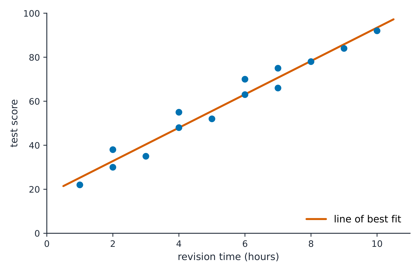
Here is one class on a scatterplot: hours of revision along the bottom, test score up the side. The line of best fit climbs. But this is only one class. Take a…
English narration · English + 中文 subtitles burned in
9.1
Do Those Points Align?
Syllabus
Source: College Board AP Course and Exam Description
Students who revise longer tend to score higher, on average, in one class's data. But a class is one sample. Would another class show the same upward slope, or could the trend be an accident of who happened to be in this one? Inference for a slope answers that, and it starts from the computer output you will be handed in the exam.
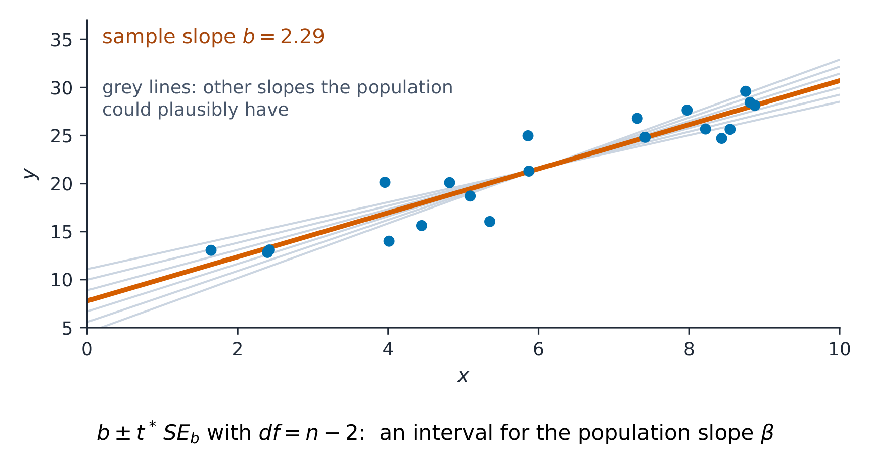
A sample scatterplot 散点图 gives a sample slope 样本斜率 $b$ for the least-squares regression line 最小二乘回归线 – but a different sample would give a slightly different slope. So $b$ is a statistic with sampling variability 抽样变异性, estimating the true (population) slope 总体斜率 $\beta$. This unit does inference 推断 for $\beta$: is there a real linear 线性 relationship, and how strong is it?
The model is $\mu_y=\alpha+\beta x$: for each $x$, the responses $y$ vary around a true line, normally and with the same standard deviation $\sigma$. Points scatter around the line partly at random. The question is whether the trend in the sample is larger than that random scatter could produce.
The sampling distribution of $b$. Over many random samples, $b$ is centred on $\beta$ (it is unbiased). Its standard deviation is estimated by
$$SE_b=\frac{s}{s_x\sqrt{n-1}},$$
where $s$ is the standard deviation of the residuals and $s_x$ the standard deviation of the $x$-values. The slope is estimated more precisely when the points sit close to the line (small $s$), when the $x$-values are spread out (large $s_x$), and when $n$ is large.
Explore
A fitted slope varies by sample
Each sample's least-squares line has a slightly different slope b.
Vocabulary
Train
| English |
|---|
| scatterplot/ˈskætəplɒt/ |
| sample slope/ˈsæmpl sləʊp/ |
| least-squares regression line/liːst skweəz rɪˈɡreʃn laɪn/ |
| sampling variability/ˈsæmplɪŋ ˌveərɪəˈbɪlɪti/ |
| true (population) slope/truː sləʊp/ |
| inference/ˈɪnfərəns/ |
| linear/ˈlɪnɪə/ |
9.2
Confidence Interval for a Slope
Syllabus
| Enduring Understanding | Learning Objective | Essential Knowledge |
|---|---|---|
UNC-4 | UNC-4.AC |
|
UNC-4.AD |
| |
UNC-4.AE |
| |
UNC-4.AF |
|
Source: College Board AP Course and Exam Description
A $t$ interval for the true slope $\beta$:
$$b\pm t^{*}\,SE_b,\qquad df=n-2,$$
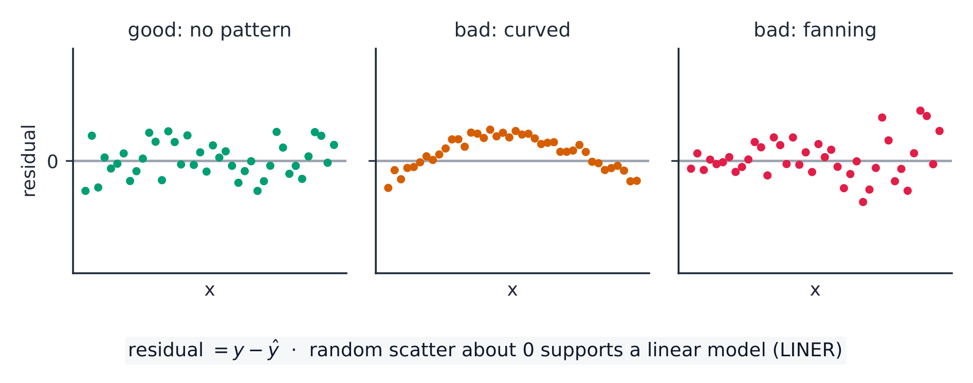
where $b$ is the sample slope and $SE_b$ its standard error 标准误 (read from computer output). Conditions 条件 (LINER): the true relationship is Linear, observations Independent, residuals 残差 Normal, and residuals have Equal spread (check the residual plot and a histogram 直方图 of residuals), from Random data. Interpret the interval for $\beta$ in context 结合情境, with units of $y$ per unit of $x$.
The residual plot 残差图 is where you check Linear and Equal-spread: you want a formless cloud around zero. A curve 曲线 means the relationship is not linear; a fan 扇形 (spread growing with $x$) means the residuals do not have equal spread – both break a condition.
Worked example. Regression output gives slope $b=2.5$ with $SE_b=0.8$ from $n=20$ points. For a $95\%$ interval, $df=18$ gives $t^*=2.101$:
$$2.5\pm2.101(0.8)=2.5\pm1.68=(0.82,\ 4.18).$$
Because $0$ is not in the interval, there is evidence of a positive linear relationship.

Explore
Inference for a regression slope
The sample slope varies from sample to sample; a confidence interval and t-test ask whether the true slope could be zero (no linear relationship).
Vocabulary
Train
| English |
|---|
| standard error/ˈstændəd ˈerə/ |
| Conditions/kənˈdɪʃnz/ |
| residuals/rɪˈsɪdʒuːəlz/ |
| histogram/ˈhɪstəɡræm/ |
| in context |
| residual plot/rɪˈsɪdʒuːəl plɒt/ |
| curve |
| fan |
9.3
Justifying a Claim About a Slope
Syllabus
| Enduring Understanding | Learning Objective | Essential Knowledge |
|---|---|---|
UNC-4 | UNC-4.AG |
|
UNC-4.AH |
| |
UNC-4.AI |
|
Source: College Board AP Course and Exam Description
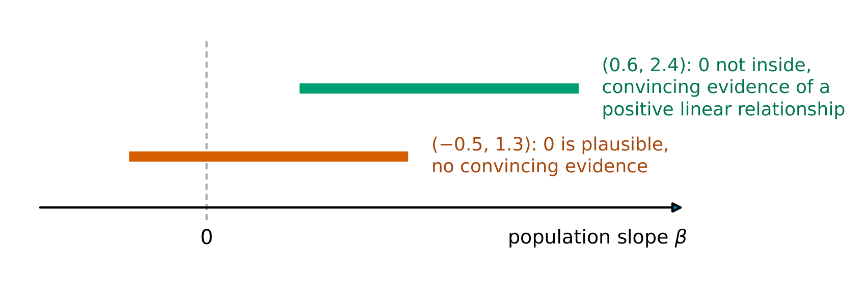
If the confidence interval 置信区间 for $\beta$ contains $0$, a slope of zero is plausible 可信 – no evidence of a linear relationship. If the interval is entirely positive or negative, there is evidence of a real (positive or negative) linear relationship. State the direction in context.
Interpreting the interval. "We are $95\%$ confident that the interval from $0.82$ to $4.18$ captures the slope of the population regression line: for each one-unit increase in $x$, the mean of $y$ increases by between $0.82$ and $4.18$ units." Larger samples give narrower intervals, other things equal.
Explore
Does the slope differ from zero?
A slope of 0 (flat line) means no linear relationship.
Vocabulary
Train
| English |
|---|
| confidence interval/ˈkɒnfɪdəns ˈɪntəvl/ |
| plausible/ˈplɔːzɪbl/ |
9.4
Setting Up a Test for a Slope
Syllabus
| Enduring Understanding | Learning Objective | Essential Knowledge |
|---|---|---|
VAR-7 | VAR-7.J |
|
VAR-7.K |
| |
VAR-7.L |
|
Source: College Board AP Course and Exam Description
The usual test asks whether there is any linear relationship:
$$H_0:\beta=0 \quad(\text{no linear relationship})\qquad H_a:\beta\neq 0 \ (\text{or } <,\,>).$$
Check the LINER conditions. This is a $t$-test on the slope.
9.5
Carrying Out a Test for a Slope
Syllabus
| Enduring Understanding | Learning Objective | Essential Knowledge |
|---|---|---|
VAR-7 | VAR-7.M |
|
DAT-3 | DAT-3.M |
|
DAT-3.N |
|
Source: College Board AP Course and Exam Description
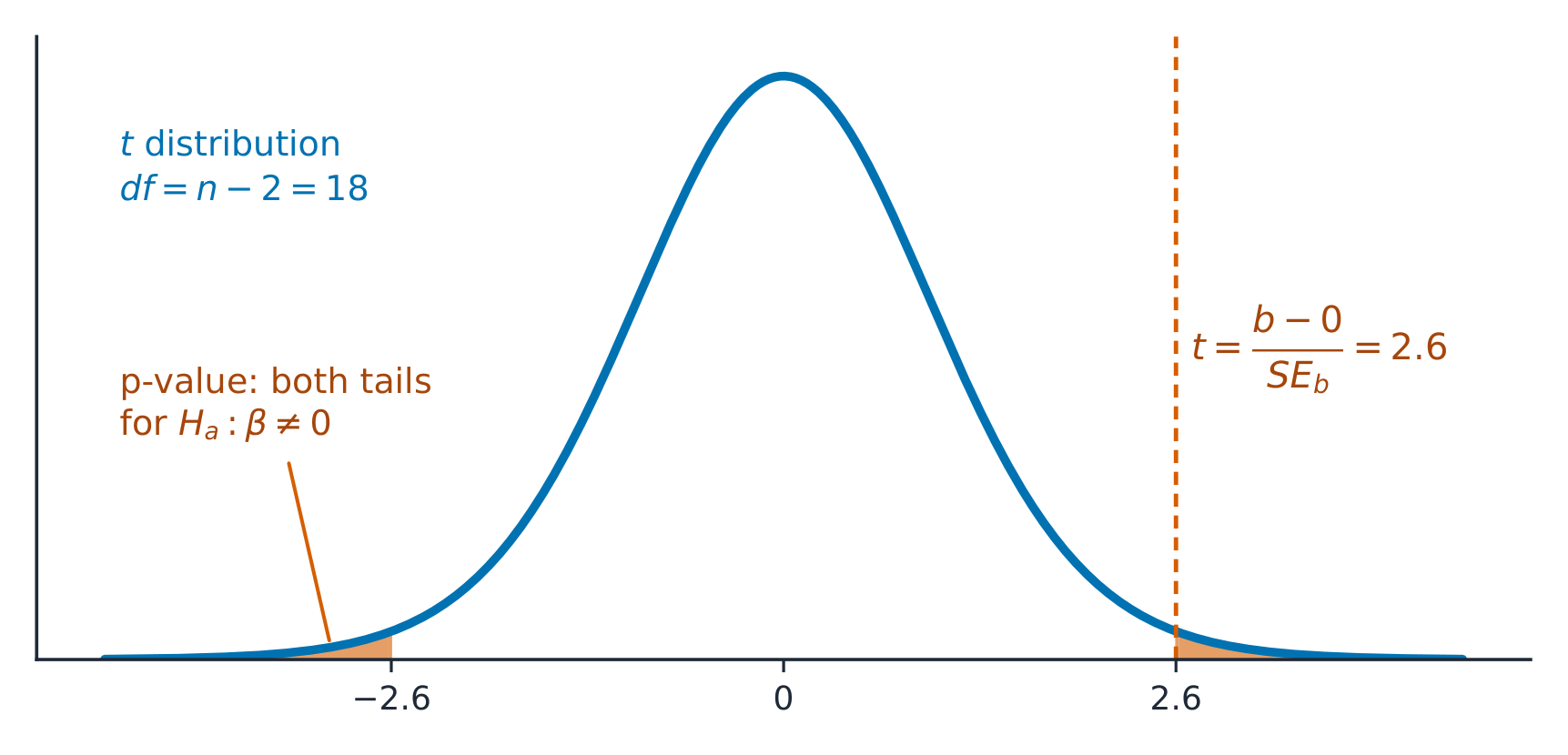
The slope $t$ statistic:
$$t=\frac{b-0}{SE_b},\qquad df=n-2.$$
Both $b$ and $SE_b$ come straight from the regression 回归 output. Find the $p$-value P值 from the $t$-distribution, compare to $\alpha$, and conclude in context – evidence (or not) of a linear relationship between the two variables.
Watch the tails. Regression output always prints the two-tailed $p$-value (for $H_a:\beta\neq 0$). If your $H_a$ is one-tailed, halve it – and first check the sample slope really points the way $H_a$ claims; if it points the other way, the one-tailed $p$-value is above $0.5$ and you cannot reject $H_0$.
Worked example. For the same output ($b=2.5$, $SE_b=0.8$, $n=20$), test $H_0:\beta=0$:
$$t=\frac{2.5-0}{0.8}=3.13,\qquad df=18,$$
a small $p$-value ($<0.01$), so reject $H_0$ – convincing evidence 有力证据 of a linear relationship. This matches the interval, which excluded $0$.
Testing a slope other than $0$. For all male sambar deer, the population slope of weight against chest circumference is $4.5\ \text{kg/cm}$. A biologist measures $20$ male tule elk and finds $b=5.4\ \text{kg/cm}$ with $SE_b=0.35$. Is the elk slope different from $4.5$? Test $H_0:\beta=4.5$ against $H_a:\beta\ne4.5$:
$$t=\frac{5.4-4.5}{0.35}=2.57,\qquad df=18,\qquad p\approx0.019.$$
Since $0.019<0.05$, reject $H_0$: there is convincing evidence that the slope for male tule elk differs from $4.5\ \text{kg/cm}$. Note that the printed $p$-value in computer output is for $\beta=0$ only; for any other value, compute $t$ yourself.
Interpreting the $p$-value. "Assuming the true slope is $4.5$, there is a $0.019$ probability of getting a sample slope at least as far from $4.5$ as $5.4$ in a random sample of $20$ elk."
Vocabulary
Train
| English |
|---|
| regression/rɪˈɡreʃn/ |
| convincing evidence |
| p-value/piː ˈvæljuː/ |
9.5
Reading regression output
Free-response questions print output like this, from a random sample of 24 students, with $x$ = hours of revision and $y$ = test score:
| Predictor | Coef | SE Coef | T | P |
|---|---|---|---|---|
| Constant | 48.2 | 4.10 | 11.76 | 0.000 |
| Hours | 3.05 | 0.92 | 3.32 | 0.003 |
$S=6.84$ and $R\text{-}Sq=33.3\%$.
- The line: predicted score $=48.2+3.05\,(\text{hours})$. The slope row, labelled with the $x$ variable, is the one that matters for inference.
- The interval: $df=24-2=22$ and $t^*=2.074$, so $3.05\pm2.074(0.92)=3.05\pm1.91$, giving $(1.14,\ 4.96)$. We are $95\%$ confident that, for each extra hour of revision, the predicted score rises by between $1.1$ and $5.0$ points, on average, for students like these.
- The test: $t=3.05/0.92=3.32$ and the printed $p=0.003$ (two-sided 双侧). That is convincing evidence of a linear relationship between revision hours and score.
- $S$ is the typical size of a residual: predictions miss by about $6.8$ points. (From $SE_b=\dfrac{s}{s_x\sqrt{n-1}}$, the revision hours had $s_x=\dfrac{6.84}{0.92\sqrt{23}}\approx1.55$ hours.) $R^2$: $33.3\%$ of the variation in scores is explained by the linear relationship with hours. The rest comes from everything else.
This was an observational 观察性的 sample, not an experiment 实验. The evidence shows an association 关联, not that revising causes higher scores: more motivated students might both revise longer and score higher.
Common mistakes. Reading the Constant row instead of the slope row; using $df=n-1$ instead of $n-2$; taking $S=6.84$ as the standard error of the slope (that is $SE_b=0.92$, in the SE Coef column); writing hypotheses about $b$ (the sample slope) instead of $\beta$; and halving the printed $p$-value when $H_a$ is two-sided.
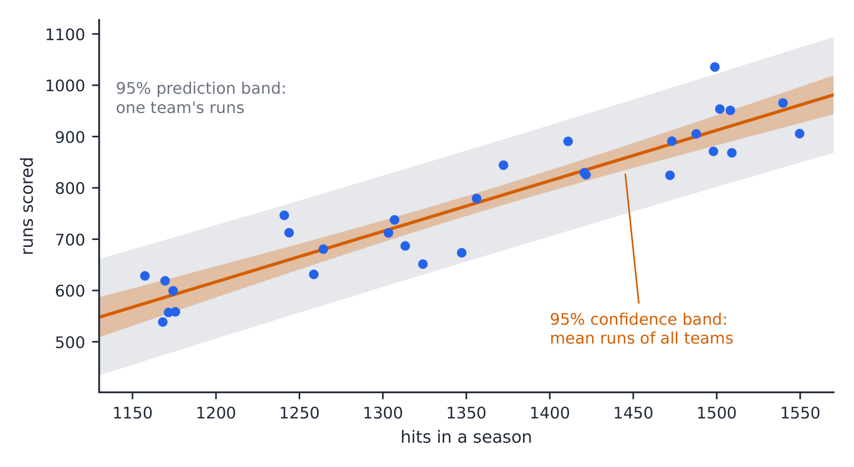
Two other intervals. Regression software can also give an interval for a predicted value. They answer different questions:
- a confidence interval for the mean response estimates the mean $y$ of all individuals with a given $x$;
- a prediction interval estimates the $y$ of one new individual with that $x$, so it must also allow for that individual's scatter about the line, and it is always wider.
Worked example. For $30$ teams, the line predicts $683$ runs for a team with $1250$ hits. Software gives $SE=17.48$ for the mean response and $SE=56.78$ for a single prediction; $df=28$ gives $t^*=2.048$.
- Mean runs for all teams with $1250$ hits: $683\pm2.048(17.48)=683\pm35.8$, so $(647,\ 719)$ runs.
- Runs for one team with $1250$ hits: $683\pm2.048(56.78)=683\pm116.3$, so $(567,\ 799)$ runs.
Vocabulary
Train
| English |
|---|
| two-sided |
| observational |
| experiment/ekˈsperɪmənt/ |
| association/əˌsəʊsɪˈeɪʃn/ |
9.6
Selecting the Right Procedure
Syllabus
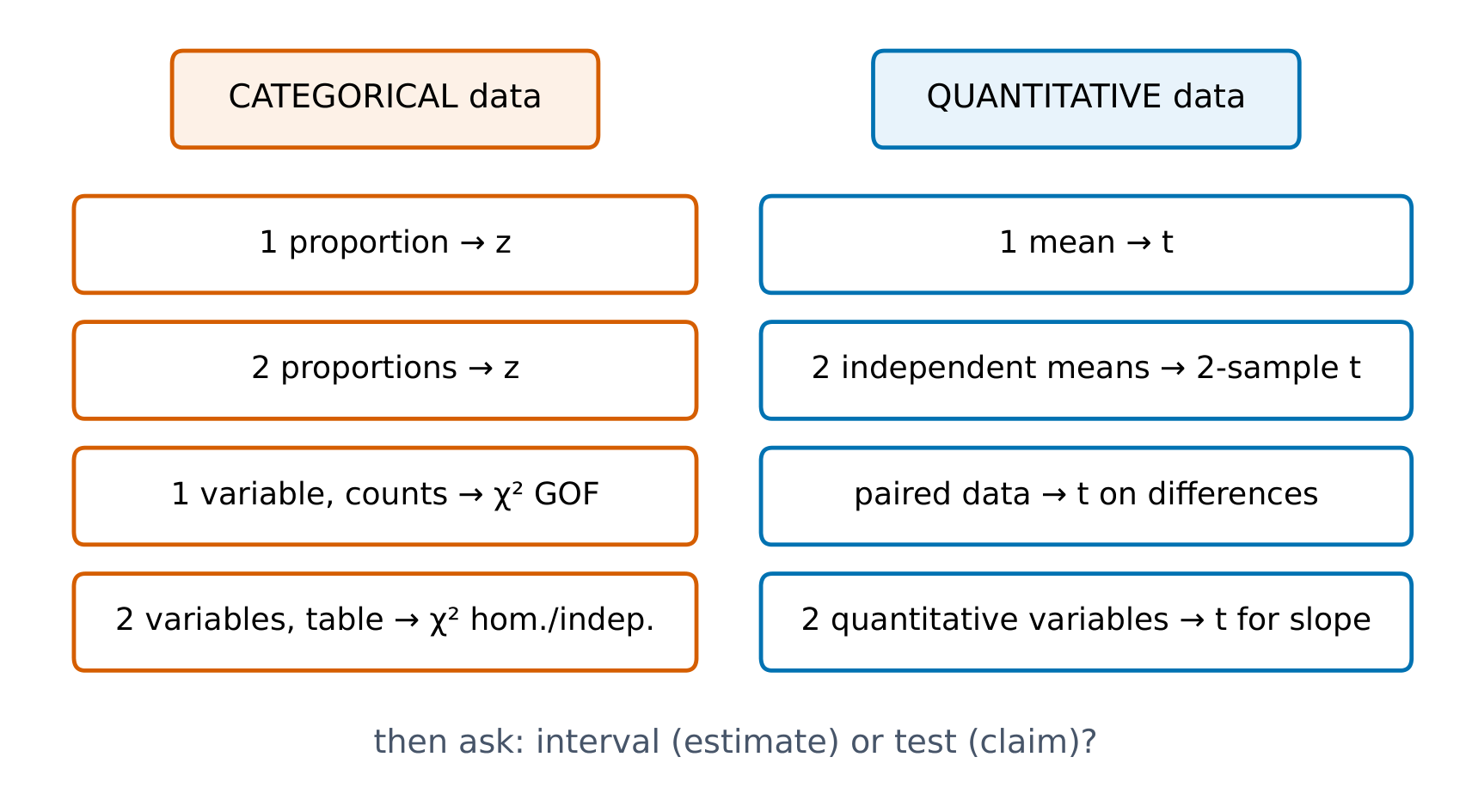
This topic is intended to focus on the skill of selecting an appropriate inference procedure now that students have a range of options. Students should be given opportunities to practice when and how to apply all learning objectives relating to inference.
Source: College Board AP Course and Exam Description
Across all of inference, identify: what is estimated or claimed (a proportion, a mean, a difference, a distribution of counts, or a slope), how many samples, and which design (independent or paired 配对; sample or experiment). Then name the procedure 检验方法, verify its conditions, carry it out, and communicate the conclusion with the statistic, the $p$-value or interval, and a plain-language answer in context. This selecting-and-communicating skill is what the investigative-task question rewards most.
Vocabulary
Train
| English |
|---|
| paired/peəd/ |
| procedure/prəˈsiːdʒə/ |
9.6
Practice
Answer each before reading the answers below. Use the output in "Reading regression output".
-
Write the equation of the least-squares line in context.
-
Predict the score of a student who revises for 6 hours.
-
Another sample of 15 points gives slope $b=-1.8$ with $SE_b=0.6$. Find the test statistic 检验统计量 and degrees of freedom 自由度 for $H_0:\beta=0$.
-
A residual plot shows a clear U-shaped curve. Which condition fails, and what does that mean for inference?
-
A student concludes from $p=0.003$: “Revising longer causes higher test scores.” Correct the student.
-
Output for $n=25$ gives $b=1.20$ with $SE_b=0.40$. Test $H_0:\beta=2$ against $H_a:\beta<2$.
-
A regression of house price on floor area is used to (a) estimate the mean price of all $120\ \text{m}^2$ houses and (b) predict the price of one particular $120\ \text{m}^2$ house. Which interval is wider, and why?
Vocabulary
Train
| English |
|---|
| test statistic/test stəˈtɪstɪk/ |
| degrees of freedom/dɪˈɡriːz ɒv ˈfriːdəm/ |
9.6
Answers
-
Predicted score $=48.2+3.05\,(\text{hours of revision})$.
-
$48.2+3.05(6)=66.5$ points.
-
$t=\dfrac{-1.8-0}{0.6}=-3.0$, with $df=15-2=13$.
-
The Linear condition fails: the true relationship is curved, so a slope interval or test for a straight line is not valid. A transformation or a different model is needed first.
-
The students were sampled, not randomly assigned to revise for different times, so this is observational data. The small $p$-value is convincing evidence of an association only. A confounding variable such as motivation could explain both.
-
$t=\dfrac{1.20-2}{0.40}=-2.0$ with $df=23$; one-sided $p\approx0.029$. At $\alpha=0.05$, reject $H_0$: convincing evidence that the true slope is less than $2$.
-
(b), the prediction interval. It must cover the price of one house, which varies around the line by about $s$, as well as the uncertainty in the line itself.
9.6
Exam tips
- Inference for a slope tests whether the true slope is $0$ (no linear relationship).
- If a slope's confidence interval includes 0, you cannot conclude a real linear relationship – the variables may still be related in a curved way.
- Read the slope, standard error, t-statistic, and p-value from the regression output. For a one-sided alternative, halve the usual two-sided p-value only when the observed slope points in the alternative's direction; otherwise use one minus half that p-value.
- Check the regression conditions (linearity, independence, roughly normal residuals, equal spread) via the residual plot.
- Interpret the interval and test in context, tied to the true slope.
- The printed $t$ and $p$ test $\beta=0$; to test another value $\beta_0$, compute $t=\dfrac{b-\beta_0}{SE_b}$ yourself.
- A prediction interval (one individual) is always wider than a confidence interval for the mean response at the same $x$.
Interactive lessons on this topic
Work through it step by step, with instant-check exercises.