Skip to content · ⁨דלג לתוכן⁩
Subjects · ⁨נושאים⁩

AP Statistics · ⁨סטטיסטיקה - AP⁩

Tips · ⁨טיפים⁩

סטטיסטיקה AP מכסה חקר נתונים, דגימה ועיצוב ניסויים, הסתברות ומשתנים מקריים, חלוקות דגימה, וסקירה – רווחי ביטחון ובדיקות מובהקות. יש מעט אלגברה; הקושי טמון באמירה הנכונה לגבי אי-ודאות.

כל תשובת סקירה מורכבת מארבעה חלקים: שמו את השיטה, בדקו את התנאים, חשבו, והסיקו בהקשר עם קישור להיפותזת החלופית. הקריטריון מדרג את הארבעה, ולכן p-value נכון לבדו מביא ציון נמוך.

השפה מוערכת. "אנו דוחים את H₀" אינו "אנו מוכיחים את H₁"; רווח ביטחון עוסק בהתנהגות ארוכת הטווח של השיטה, ולא בהסתברות שהרווח הספציפי מכיל את הפרמטר. הבחנות אלו קובעות את הנקודות.

ההערות עוברות על כל התשע היחידות כאשר כל שיטת סקירה מוצגת צעד אחר צעד. FRQs שפורסמו זמינים בספרייה. סטטיסטיקה מביאה נקודות על ניסוח התנאים ופרשנות בהקשר, ולכן כל תשובה מופרשת מוזכרת את התנאים לפני שהיא מבצעת את הבדיקה.

  • 1

    Exploring One-Variable Data · ⁨חקר נתוני משתנה אחד⁩

    Watch lesson · ⁨צפה בשיעור⁩
    1.1

    Introducing Statistics: What Can We Learn from Data?

    Syllabus · ⁨סיילבוס⁩
    English

    Enduring Understanding (VAR-1): Given that variation may be random or not, conclusions are uncertain.

    Learning Objective VAR-1.A: Identify questions to be answered, based on variation in one-variable data. [Skill 1.A]

    • VAR-1.A.1 Numbers may convey meaningful information, when placed in context.
    עברית

    הבנה מתמשכת (VAR-1): בשל כך ששינוי עשוי להיות אקראי או לא, המסקנות הן לא וודאות.

    מטרות למידה VAR-1.A: זיהוי שאלות לענות עליהן, על בסיס שינוי בנתוני משתנה אחד. [מיומנות 1.A]

    • VAR-1.A.1 מספרים עשויים להעביר מידע משמעותי, כאשר הם ממוקמים בהקשר.
    Source: College Board AP Course and Exam Description · ⁨מקור: תיאור הקורס והמבחן של College Board AP⁩

    Statistics 统计学 is the science of learning from data 数据 – numbers or labels collected from the real world. Data vary, so we describe patterns and account for the variation 变异 rather than expecting every value to match. A statistical question anticipates an answer based on data that vary.

    Two distinctions run through the whole course. A parameter 参数 is a numerical summary of a whole population; a statistic 统计量 is a numerical summary of a sample - we use the statistic to estimate the parameter we cannot measure directly. And descriptive statistics 描述统计 only summarise the data set in hand, while inferential statistics 推断统计 use a sample to make and test claims about the larger population.

    Vocabulary · ⁨מילון מונחים⁩ Train · ⁨אימון⁩
    English עברית
    Statistics/stəˈtɪstɪks/ סטטיסטיקה
    data/ˈdeɪtə/ נתונים
    variation/ˌveərɪˈeɪʃn/ וריאות
    parameter/pəˈræmɪtə/ פרמטר
    statistic/stəˈtɪstɪk/ סטטיסטיקה
    descriptive statistics/dɪˈskrɪptɪv stəˈtɪstɪks/ סטטיסתיים תיאוריים
    inferential statistics/ɪnfəˈrenʃl stəˈtɪstɪks/ סטטיסטיקה אינפראנציה (מסקנתית)
    1.2

    The Language of Variation: Variables

    Syllabus · ⁨סיילבוס⁩
    English

    Enduring Understanding (VAR-1): Given that variation may be random or not, conclusions are uncertain.

    Learning Objective VAR-1.B: Identify variables in a set of data. [Skill 2.A]

    • VAR-1.B.1 A variable is a characteristic that changes from one individual to another.

    Learning Objective VAR-1.C: Classify types of variables. [Skill 2.A]

    • VAR-1.C.1 A categorical variable takes on values that are category names or group labels.
    • VAR-1.C.2 A quantitative variable is one that takes on numerical values for a measured or counted quantity.
      • Illustrative examples for VAR-1.C:
        • Categorical variables:
          • Dominant hand
          • Age group (young or old)
          • Highest degree earned
        • Quantitative variables:
          • Age of a structure
          • Height of a child
          • Concentration of a sample
    עברית

    הבנה מתמשכת (VAR-1): בשל כך ששינוי עשוי להיות אקראי או לא, המסקנות הן לא וודאות.

    מטרת הלמידה VAR-1.B: זיהוי משתנים בקבוצת נתונים. [מיומנות 2.A]

    • VAR-1.B.1 משתנה הוא תכונה השונה מאדם אחד לאחר.

    מטרת הלמידה VAR-1.C: סיווג סוגי משתנים. [מיומנות 2.A]

    • VAR-1.C.1 משתנה קטגוריאלי מקבל ערכים שהם שמות קטגוריות או תוויות קבוצות.
    • VAR-1.C.2 משתנה כמותי הוא משתנה המקבל ערכים מספריים לכמות שנמדדה או נספרה.
      • דוגמאות מדגמות עבור VAR-1.C:
        • משתנים קטגוריאליים:
          • יד דומיננטית
          • קבוצת גיל (צעיר או זקן)
          • התואר הגבוה ביותר שהושג
        • משתנים כמותיים:
          • גיל מבנה
          • גובה ילד
          • ריכוז הדוגמה

    Source: College Board AP Course and Exam Description · ⁨מקור: תיאור הקורס והמבחן של College Board AP⁩

    A variable 变量 is a characteristic that can differ between individuals. Two kinds:

    • Categorical 分类 (qualitative): values are labels/groups (eye colour, brand).
    • Quantitative 定量: values are numbers you can do arithmetic on (height, age). Quantitative variables are discrete (countable) or continuous (measured).

    Choosing the right graph and summary depends on which kind you have.

    Explore · ⁨חקור⁩

    Categorical or quantitative?

    Every variable is either categorical (it labels each unit with a group) or quantitative (a measured number you can average). Which kind it is decides the graphs and summaries you are allowed to use.

    Vocabulary · ⁨מילון מונחים⁩ Train · ⁨אימון⁩
    English עברית
    variable/ˈveərɪəbl/ משתנה
    Categorical/ˌkætɪˈɡɒrɪkl/ קטגוריאלי
    Quantitative/ˈkwɒntɪteɪtɪv/ כמותי
    1.3

    Representing a Categorical Variable with Tables

    Syllabus · ⁨סיילבוס⁩
    English

    Enduring Understanding (UNC-1): Graphical representations and statistics allow us to identify and represent key features of data.

    Learning Objective UNC-1.A: Represent categorical data using frequency or relative frequency tables. [Skill 2.B]

    • UNC-1.A.1 A frequency table gives the number of cases falling into each category. A relative frequency table gives the proportion of cases falling into each category.

    Learning Objective UNC-1.B: Describe categorical data represented in frequency or relative tables. [Skill 2.A]

    • UNC-1.B.1 Percentages, relative frequencies, and rates all provide the same information as proportions.
    • UNC-1.B.2 Counts and relative frequencies of categorical data reveal information that can be used to justify claims about the data in context.
    עברית

    הבנה מתמשכת (UNC-1): ייצוגים גרפיים וסטטיסטיקה מאפשרים לזהות ולייצג תכונות מרכזיות של נתונים.

    מטרות למידה UNC-1.A: ייצוג נתונים קטגוריאליים באמצעות טבלאות תדירות או תדירות יחסית. [מיומנות 2.B]

    • UNC-1.A.1 טבלת תדירות מציגה את מספר המקרים הנופלים בכל קטגוריה. טבלת תדירות יחסית מציגה את הפרופורציה של המקרים הנופלים בכל קטגוריה.

    מטרות למידה UNC-1.B: תיאור נתונים קטגוריאליים המוצגים בטבלאות תדירות או תדירות יחסית. [מיומנות 2.A]

    • UNC-1.B.1 אחוזים, תדירויות יחסיות ומדדים מספקים את אותה מידע כמו פרופורציות.
    • UNC-1.B.2 ספירות ותדירויות יחסיות של נתונים קטגוריאליים חושפות מידע שיכול לשמש להנמנת טענות לגבי הנתונים בהקשר.
    Source: College Board AP Course and Exam Description · ⁨מקור: תיאור הקורס והמבחן של College Board AP⁩

    A frequency table 频数表 lists each category's count (frequency); a relative frequency 相对频率 table lists each category's proportion 比例 (count ÷ total). Relative frequencies let you compare groups of different sizes fairly.

    Vocabulary · ⁨מילון מונחים⁩ Train · ⁨אימון⁩
    English עברית
    frequency table/ˈfriːkwənsi ˈteɪbl/ טבלת תדירות
    relative frequency/ˈrelətɪv ˈfriːkwənsi/ תדירות יחסית
    proportion/prəˈpɔːʃn/ יחסים פרופורציונליים
    1.4

    Representing a Categorical Variable with Graphs

    Syllabus · ⁨סיילבוס⁩
    English

    Enduring Understanding (UNC-1): Graphical representations and statistics allow us to identify and represent key features of data.

    Learning Objective UNC-1.C: Represent categorical data graphically. [Skill 2.B]

    • UNC-1.C.1 Bar charts (or bar graphs) are used to display frequencies (counts) or relative frequencies (proportions) for categorical data.
    • UNC-1.C.2 The height or length of each bar in a bar graph corresponds to either the number or proportion of observations falling within each category.
    • UNC-1.C.3 There are many additional ways to represent frequencies (counts) or relative frequencies (proportions) for categorical data.

    Learning Objective UNC-1.D: Describe categorical data represented graphically. [Skill 2.A]

    • UNC-1.D.1 Graphical representations of a categorical variable reveal information that can be used to justify claims about the data in context.

    Learning Objective UNC-1.E: Compare multiple sets of categorical data. [Skill 2.D]

    • UNC-1.E.1 Frequency tables, bar graphs, or other representations can be used to compare two or more data sets in terms of the same categorical variable.
    עברית

    הבנה מתמשכת (UNC-1): ייצוגים גרפיים וסטטיסטיקה מאפשרים לזהות ולייצג תכונות מרכזיות של נתונים.

    מטרות למידה UNC-1.C: ייצוג נתונים קטגוריאליים גרפית. [מיומנות 2.B]

    • UNC-1.C.1 גרפי עמודות (או גרפי פס) משמשים להצגת תדירויות (ספירות) או תדירויות יחסיות (פרופורציות) עבור נתונים קטגוריאליים.
    • UNC-1.C.2 הגובה או האורך של כל עמודה בגרף עמודות מתאימים לספירה או לפרופורציה של הצפות הנופלות בתוך כל קטגוריה.
    • UNC-1.C.3 קיימות דרכים נוספות רבות לייצוג תדירויות (ספירות) או תדירויות יחסיות (פרופורציות) עבור נתונים קטגוריאליים.

    מטרות למידה UNC-1.D: תיאור נתונים קטגוריאליים המוצגים גרפית. [מיומנות 2.A]

    • UNC-1.D.1 ייצוגים גרפיים של משתנה קטגוריאלי חושפים מידע שיכול לשמש להנמנת טענות לגבי הנתונים בהקשר.
    מטרות למידה UNC-1.E: השוואת מספר קבוצות נתונים קטגוריאליים. [מיומנות 2.D]

    • UNC-1.E.1 טבלאות תדירות, גרפי עמודות או ייצוגים אחרים יכולים לשמש להשוואה בין שתי קבוצות נתונים או יותר על פי אותו משתנה קטגוריאלי.

    Source: College Board AP Course and Exam Description · ⁨מקור: תיאור הקורס והמבחן של College Board AP⁩

    Bar charts 条形图 show the count or proportion of each category as separated bars; a pie chart shows each category's share of the whole. The bar heights (or slices) let you compare categories at a glance. Bars may be ordered by size or by a natural category order.

    Explore · ⁨חקור⁩

    Show a categorical variable as a pie chart

    A pie chart turns each category's share of the whole into a slice: a bigger share is a bigger slice, and every slice together makes 100%. It is a picture of a relative-frequency table.

    Vocabulary · ⁨מילון מונחים⁩ Train · ⁨אימון⁩
    English עברית
    Bar charts/bɑː tʃɑːts/ גרפים עמודתיים
    1.5

    Representing a Quantitative Variable with Graphs

    Syllabus · ⁨סיילבוס⁩
    English

    Enduring Understanding (UNC-1): Graphical representations and statistics allow us to identify and represent key features of data.

    Learning Objective UNC-1.F: Classify types of quantitative variables. [Skill 2.A]

    • UNC-1.F.1 A discrete variable can take on a countable number of values. The number of values may be finite or countably infinite, as with the counting numbers.
    • UNC-1.F.2 A continuous variable can take on infinitely many values, but those values cannot be counted. No matter how small the interval between two values of a continuous variable, it is always possible to determine another value between them.
      • Illustrative examples for UNC-1.F:
        • A discrete variable:
          • Number of students in a class
        • A continuous variable:
          • Height of a child

    Learning Objective UNC-1.G: Represent quantitative data graphically. [Skill 2.B]

    • UNC-1.G.1 In a histogram, the height of each bar shows the number or proportion of observations that fall within the interval corresponding to that bar. Altering the interval widths can change the appearance of the histogram.
    • UNC-1.G.2 In a stem and leaf plot, each data value is split into a "stem" (the first digit or digits) and a "leaf" (usually the last digit).
    • UNC-1.G.3 A dotplot represents each observation by a dot, with the position on the horizontal axis corresponding to the data value of that observation, with nearly identical values stacked on top of each other.
    • UNC-1.G.4 A cumulative graph represents the number or proportion of a data set less than or equal to a given number.
    • UNC-1.G.5 There are many additional ways to graphically represent distributions of quantitative data.
    עברית

    הבנה מתמשכת (UNC-1): ייצוגים גרפיים וסטטיסטיקה מאפשרים לזהות ולייצג תכונות מרכזיות של נתונים.

    מטרות למידה UNC-1.F: סיווג סוגי משתנים כמותיים. [מיומנות 2.A]

    • UNC-1.F.1 משתנה דיסקרטי יכול לקבל מספר ספיר של ערכים. מספר הערכים עשוי להיות סופי או אינסופי ספיר, כמו במספרי הספירה.
    • UNC-1.F.2 משתנה רציף יכול לקבל ערכים אינסופיים, אך ערכים אלו אינם ספריים. ללא תלות בגודל המרווח בין שני ערכים של משתנה רציף, תמיד ניתן למצוא ערך נוסף ביניהם.
      • דוגמאות להמחשה עבור UNC-1.F:
        • משתנה בדיד:
          • מספר תלמידים בכיתה
        • משתנה רציף:
          • גובה ילד

    מטרת הלמידה UNC-1.G: ייצוג נתונים כמותיים גרפית. [מיומנות 2.B]

    • UNC-1.G.1 בהיסטוגרמה, גובהו של כל עמודה מייצג את מספר או את היחס של הנתונים הנופלים בתוך המרווח המתאים לעמודה זו. שינוי רוחב המרווחים עלול לשנות את מראה ההיסטוגרמה.
    • UNC-1.G.2 במסדרת גבעות ועלים, כל ערך נתון מחולק ל"גבעה" (הספרה הראשונה או הספרות הראשונות) ול"עלה" (בדרך כלל הספרה האחרונה).
    • UNC-1.G.3 דיאגרמת נקודות מייצגת כל תצפית באמצעות נקודה, כאשר המיקום על הציר האופקי מתאים לערך הנתון של התצפית זו, כאשר ערכים זהים כמעט ערוכים אחד מעל השני.
    • UNC-1.G.4 גרף מצטבר מייצג את מספר או את היחס של נתונים קטניםים או שווים לערך נתון.
    • UNC-1.G.5 קיימים עוד דרכים רבות ליצוג גרפי של חלוקות נתונים כמותיים.

    Source: College Board AP Course and Exam Description · ⁨מקור: תיאור הקורס והמבחן של College Board AP⁩

    For numbers, use a dotplot 点图, stem-and-leaf plot 茎叶图, or histogram 直方图 (bars over value intervals called bins). These show the distribution 分布 – how the values spread out. A histogram's bin width changes the picture, so choose it to reveal the shape.

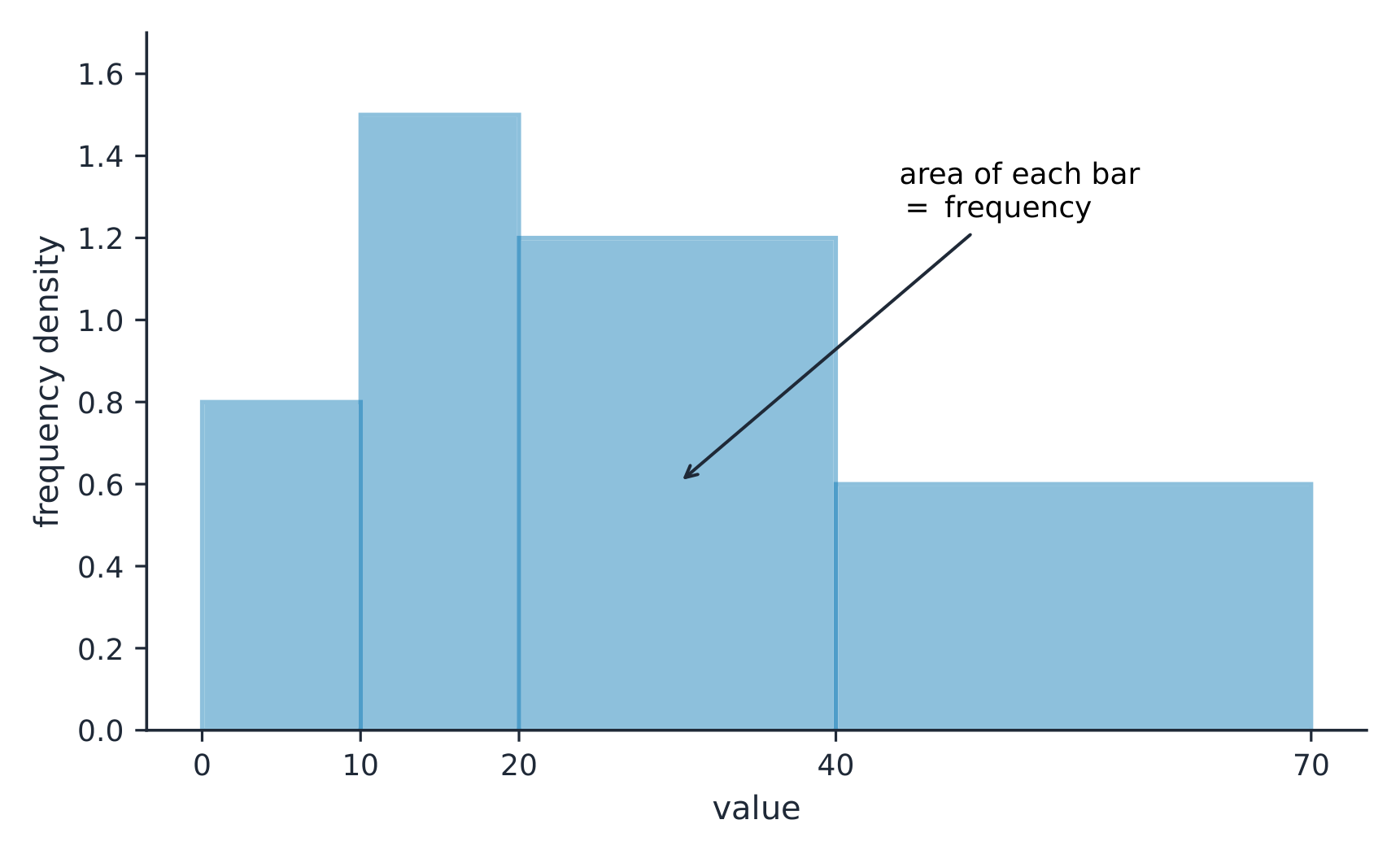
    On a histogram with unequal class widths the bar area is the frequency
    On a histogram with unequal class widths the bar area is the frequency
    Explore · ⁨חקור⁩

    Explore how bin width shapes a histogram

    A histogram groups data into equal-width bins and draws a bar over each. Change the bins and notice how the same data can look jagged (too narrow) or smooth (too wide) — the shape is a choice.

    Vocabulary · ⁨מילון מונחים⁩ Train · ⁨אימון⁩
    English עברית
    dotplot/ˈdɒtplɒt/ תרשים נקודות
    stem-and-leaf plot/stem ænd liːf plɒt/ תרשימת גבעה ועלים
    histogram/ˈhɪstəɡræm/ היסטוגרמה
    distribution/ˌdɪstrɪˈbjuːʃn/ חלוקה
    1.6

    Describing the Distribution of a Quantitative Variable

    Syllabus · ⁨סיילבוס⁩
    English

    Enduring Understanding (UNC-1): Graphical representations and statistics allow us to identify and represent key features of data.

    Learning Objective UNC-1.H: Describe the characteristics of quantitative data distributions. [Skill 2.A]

    • UNC-1.H.1 Descriptions of the distribution of quantitative data include shape, center, and variability (spread), as well as any unusual features such as outliers, gaps, clusters, or multiple peaks.
    • UNC-1.H.2 Outliers for one-variable data are data points that are unusually small or large relative to the rest of the data.
    • UNC-1.H.3 A distribution is skewed to the right (positive skew) if the right tail is longer than the left. A distribution is skewed to the left (negative skew) if the left tail is longer than the right. A distribution is symmetric if the left half is the mirror image of the right half.
    • UNC-1.H.4 Univariate graphs with one main peak are known as unimodal. Graphs with two prominent peaks are bimodal. A graph where each bar height is approximately the same (no prominent peaks) is approximately uniform.
    • UNC-1.H.5 A gap is a region of a distribution between two data values where there are no observed data.
    • UNC-1.H.6 Clusters are concentrations of data usually separated by gaps.
    • UNC-1.H.7 Descriptive statistics does not attribute properties of a data set to a larger population, but may provide the basis for conjectures for subsequent testing.
    עברית

    הבנה מתמשכת (UNC-1): ייצוגים גרפיים וסטטיסטיקה מאפשרים לזהות ולייצג תכונות מרכזיות של נתונים.

    מטרת הלמידה UNC-1.H: תיאור מאפייני חלוקות נתונים כמותיים. [מיומנות 2.A]

    • UNC-1.H.1 תיאורים של חלוקת נתונים כמותיים כוללים צורה, מרכזיות ושיבוש (פיזור), כמו גם מאפיינים בולטים כלשהם כגון ערכים קיצוניים, רווחים, צבירים או פסגות מרובות.
    • UNC-1.H.2 ערכים קיצוניים לנתוני משתנה אחד הם נקודות נתונים שהן קטנות או גדולות בצורה בולטת ביחס לשאר הנתונים.
    • UNC-1.H.3 חלוקה היא אלכסונית ימינה (אלכסון חיובי) אם הזנב הימני ארוך מהשמאלי. חלוקה היא אלכסונית שמאלה (אלכסון שלילי) אם הזנב השמאלי ארוך מימני. חלוקה היא סימטרית אם החלק השמאלי הוא תמונת ראי של החלק הימני.
    • UNC-1.H.4 גרפים חד-משתניים עם פסגה אחת ראשית נקראים חד-פסגתיים. גרפים עם שתי פסגות בולטות הם דו-פסגתיים. גרף בו גובה העמודות הוא בערך זהה (ללא פסגות בולטות) הוא בערך אחיד.
    • UNC-1.H.5 רווח הוא אזור בחלוקה בין שני ערכי נתונים שאין בו נתונים שנצפו.
    • UNC-1.H.6 צבירים הם ריכוזי נתונים המופרדים בדרך כלל על ידי רווחים.
    • UNC-1.H.7 סטטיסטיקה תיאורית אינה יחסה מאפיינים של קבוצת נתונים לאוכלוסייה רחבה יותר, אך עשויה לספק בסיס לניחוחות לבדיקות בעתיד.

    Source: College Board AP Course and Exam Description · ⁨מקור: תיאור הקורס והמבחן של College Board AP⁩

    Describe four things (remember SOCS):

    • Shape 形状: symmetric, or skewed 偏斜 left/right (a long tail on that side), and how many peaks - one main peak is unimodal 单峰, two prominent peaks bimodal 双峰, and roughly equal bars uniform 均匀.
    • Outliers 离群值: unusual values far from the rest.
    • Center: a typical value (mean or median).
    • Spread: how much the values vary (range, IQR, standard deviation).

    Always describe shape/center/spread in context, with units.

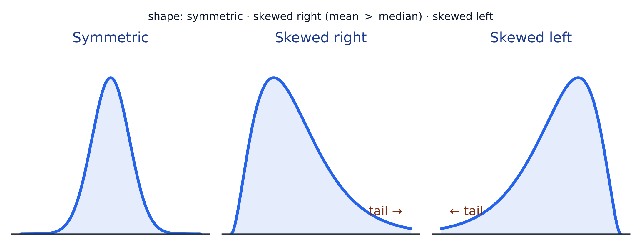
    The shape of a distribution: symmetric, skewed right (long right tail), or skewed left
    The shape of a distribution: symmetric, skewed right (long right tail), or skewed left
    Vocabulary · ⁨מילון מונחים⁩ Train · ⁨אימון⁩
    English עברית
    Shape/ʃeɪp/ צורה
    skewed/skjuːd/ עיוות (שיפוע)
    unimodal/ˌʌnɪˈmɒdl/ חד-שיא
    bimodal/baɪˈmɒdl/ דו-שיאי
    uniform/ˈjuːnɪfɔːm/ אחיד
    Outliers/ˈaʊtlaɪəz/ ערכים קיצוניים
    1.7

    Summary Statistics for a Quantitative Variable

    Syllabus · ⁨סיילבוס⁩
    English

    Enduring Understanding (UNC-1): Graphical representations and statistics allow us to identify and represent key features of data.

    Learning Objective UNC-1.I: Calculate measures of center and position for quantitative data. [Skill 2.C]

    • UNC-1.I.1 A statistic is a numerical summary of sample data.
    • UNC-1.I.2 The mean is the sum of all the data values divided by the number of values. For a sample, the mean is denoted by $x$-bar: $\bar{x} = \dfrac{1}{n}\sum_{i=1}^{n} x_i$, where $x_i$ represents the $i^{\text{th}}$ data point in the sample and $n$ represents the number of data values in the sample.
    • UNC-1.I.3 The median of a data set is the middle value when data are ordered. When the number of data points is even, the median can take on any value between the two middle values. In AP Statistics, the most commonly used value for the median of a data set with an even number of values is the average of the two middle values.
    • UNC-1.I.4 The first quartile, Q1, is the median of the half of the ordered data set from the minimum to the position of the median. The third quartile, Q3, is the median of the half of the ordered data set from the position of the median to the maximum. Q1 and Q3 form the boundaries for the middle 50% of values in an ordered data set.
    • UNC-1.I.5 The $p^{\text{th}}$ percentile is interpreted as the value that has $p\%$ of the data less than or equal to it.

    Learning Objective UNC-1.J: Calculate measures of variability for quantitative data. [Skill 2.C]

    • UNC-1.J.1 Three commonly used measures of variability (or spread) in a distribution are the range, interquartile range, and standard deviation.
    • UNC-1.J.2 The range is defined as the difference between the maximum data value and the minimum data value. The interquartile range (IQR) is defined as the difference between the third and first quartiles: $Q3 - Q1$. Both the range and the interquartile range are possible ways of measuring variability of the distribution of a quantitative variable.
    • UNC-1.J.3 Standard deviation is a way to measure variability of the distribution of a quantitative variable. For a sample, the standard deviation is denoted by $s$: $s_x = \sqrt{\dfrac{1}{n-1}\sum(x_i - \bar{x})^2}$. The square of the sample standard deviation, $s^2$, is called the sample variance.
    • UNC-1.J.4 Changing units of measurement affects the values of the calculated statistics.

    Learning Objective UNC-1.K: Explain the selection of a particular measure of center and/or variability for describing a set of quantitative data. [Skill 4.B]

    • UNC-1.K.1 There are many methods for determining outliers. Two methods frequently used in this course are:
      • UNC-1.K.1.i An outlier is a value greater than $1.5 \times \text{IQR}$ above the third quartile or more than $1.5 \times \text{IQR}$ below the first quartile.
      • UNC-1.K.1.ii An outlier is a value located 2 or more standard deviations above, or below, the mean.
    • UNC-1.K.2 The mean, standard deviation, and range are considered nonresistant (or non-robust) because they are influenced by outliers. The median and IQR are considered resistant (or robust), because outliers do not greatly (if at all) affect their value.
    עברית

    הבנה מתמשכת (UNC-1): ייצוגים גרפיים וסטטיסטיקה מאפשרים לזהות ולייצג תכונות מרכזיות של נתונים.

    מטרות לימוד UNC-1.I: חשב מידות מרכז ומיקום לנתונים כמותיים. [מיומנות 2.C]

    • UNC-1.I.1 סטטיסטיקה היא סיכום מספרי של נתוני דוגמה.
    • UNC-1.I.2 הממוצע הוא סכום כל ערכי הנתונים מחולק במספר הערכים. לדוגמה, הממוצע מסומן על ידי $x$: $\bar{x} = \dfrac{1}{n}\sum_{i=1}^{n} x_i$, כאשר $x_i$ מייצג את ה$i^{\text{th}}$ נקודת הנתון בדוגמה ו$n$ מייצג את מספר ערכי הנתונים בדוגמה.
    • UNC-1.I.3 הניצב (המחצית) של מערך נתונים הוא הערך האמצעי כאשר הנתונים מסודרים. כאשר מספר נקודות הנתונים הוא זוגי, הניצב יכול לקבל כל ערך בין שני הערכים האמצעיים. בתרומיות AP, הערך הנפוץ ביותר עבור הניצב של מערך נתונים עם מספר זוגי של ערכים הוא הממוצע של שני הערכים האמצעיים.
    • UNC-1.I.4 הרביע הראשון, Q1, הוא הניצב של החצי ממערך הנתונים המסודר מהמינימום ועד למיקום הניצב. הרביע השלישי, Q3, הוא הניצב של החצי ממערך הנתונים המסודר ממיקום הניצב עד למקסימום. Q1 ו-Q3 יוצרים את הגבולות עבור 50% המרכזיים של ערכים במערך נתונים מסודר.
    • UNC-1.I.5 ה$p^{\text{th}}$ פרצנטיל מתורגם כערך שעבורו $p\%$ מהנתונים קטנים או שווים לו.

    מטרות לימוד UNC-1.J: חשב מידות התפלגות לנתונים כמותיים. [מיומנות 2.C]

    • UNC-1.J.1 שלושה מידות התפלגות (או פיזור) נפוצות בהתפלגות הן טווח, טווח רביעי ואי-סטינדרט.
    • UNC-1.J.2 הטווח מוגדר כהפרש בין הערך המקסימלי לערך המינימלי של הנתונים. טווח הרביעים (IQR) מוגדר כהפרש בין הרביע השלישי לרביע הראשון: $Q3 - Q1$. גם הטווח וגם טווח הרביעים הם דרכים אפשריות למדוד את ההתפלגות של משתנה כמותי.
    • UNC-1.J.3 אי-סטינדרט הוא דרך למדוד את ההתפלגות של משתנה כמותי. לדוגמה, האי-סטינדרט מסומן על ידי $s$: $s_x = \sqrt{\dfrac{1}{n-1}\sum(x_i - \bar{x})^2}$. ריבוע האי-סטינדרט של הדוגמה, $s^2$, נקרא וاریאנס הדוגמה.
    • UNC-1.J.4 שינוי יחידות המדידה משפיע על ערכי הסטטיסטיקות המחושבות.

    מטרות לימוד UNC-1.K: הסבר הבחירה במידת מרכז ו/או התפלגות ספציפית לתיאור מערך נתונים כמותי. [מיומנות 4.B]

    • UNC-1.K.1 קיימות שיטות רבות לזיהוי ערכים קיצוניים. שתי שיטות הנפוצות בקורס זה הן:
      • UNC-1.K.1.i ערך קיצוני הוא ערך גדול ב-$1.5 \times \text{IQR}$ מעל הרביע השלישי או יותר מ-$1.5 \times \text{IQR}$ מתחת לרביע הראשון.
      • UNC-1.K.1.ii ערך קיצוני הוא ערך הנמצא 2 או יותר אי-סטינדרטים מעל או מתחת לממוצע.
    • UNC-1.K.2 הממוצע, האי-סטינדרט והטווח נחשבים ללא-עמידים (או לא-רובסטיים) משום שהם מושפעים מערכים קיצוניים. הניצב וה-IQR נחשבים לעמידים (או רובסטיים), משום שערכים קיצוניים אינם משפיעים עליהם באופן משמעותי (אם בכלל על ערכם).

    Source: College Board AP Course and Exam Description · ⁨מקור: תיאור הקורס והמבחן של College Board AP⁩

    Standard deviation: spread about the mean
    • Center: the mean 均值 $\bar{x}=\dfrac{\sum x_i}{n}$ (average) and the median 中位数 (middle value). The median resists outliers; the mean is pulled toward a skew.
    • Spread: the range, the interquartile range 四分位距 $\text{IQR}=Q_3-Q_1$ (middle 50%), and the standard deviation 标准差 $s_x=\sqrt{\dfrac{\sum(x_i-\bar{x})^2}{n-1}}$ (typical distance from the mean; its square is the variance 方差).
    • The five-number summary 五数概括: min, $Q_1$, median, $Q_3$, max.

    Use resistant measures (median, IQR) for skewed data; mean and standard deviation for roughly symmetric data.

    The percentile 百分位数 of a value is the percent of the data at or below it – so the median is the 50th percentile and $Q_1$ the 25th. A cumulative relative frequency graph 累积相对频率图 makes percentiles easy to read: for each value it plots the proportion of the data at or below it, rising from 0 to 1. Go up from a value to the curve and across to its percentile, or reverse the steps to find the value at a given percentile (the same reading works from a cumulative-frequency table).

    Worked example. For the data $4, 8, 6, 10, 7$: the mean is $\bar{x}=\dfrac{4+8+6+10+7}{5}=\dfrac{35}{5}=7$. Sorting to $4,6,7,8,10$, the median is the middle value, $7$. The mean and median agree here because the data are roughly symmetric.

    Vocabulary · ⁨מילון מונחים⁩ Train · ⁨אימון⁩
    English עברית
    mean/miːn/ ממוצע
    median/ˈmiːdiːən/ חציון
    interquartile range/ˌɪntəˈkwɔːtaɪl reɪndʒ/ טווח רביעי
    standard deviation/ˈstændəd ˌdiːvɪˈeɪʃn/ סטיית תקן
    variance/ˈveərɪəns/ סטייה
    five-number summary/faɪv ˈnʌmbə ˈsʌməri/ סיכום חמישה מספרים
    percentile/pəˈsentaɪl/ אחוזון
    cumulative relative frequency graph/ˈkjuːmjʊlətɪv ˈrelətɪv ˈfriːkwənsi ɡræf/ גרף תדירות יחסית מצטברת
    1.8

    Graphical Representations of Summary Statistics

    Syllabus · ⁨סיילבוס⁩
    English

    Enduring Understanding (UNC-1): Graphical representations and statistics allow us to identify and represent key features of data.

    Learning Objective UNC-1.L: Represent summary statistics for quantitative data graphically. [Skill 2.B]

    • UNC-1.L.1 Taken together, the minimum data value, the first quartile (Q1), the median, the third quartile (Q3), and the maximum data value make up the five-number summary.
    • UNC-1.L.2 A boxplot is a graphical representation of the five-number summary (minimum, first quartile, median, third quartile, maximum). The box represents the middle 50% of data, with a line at the median and the ends of the box corresponding to the quartiles. Lines ("whiskers") extend from the quartiles to the most extreme point that is not an outlier, and outliers are indicated by their own symbol beyond this.

    Learning Objective UNC-1.M: Describe summary statistics of quantitative data represented graphically. [Skill 2.A]

    • UNC-1.M.1 Summary statistics of quantitative data, or of sets of quantitative data, can be used to justify claims about the data in context.
    • UNC-1.M.2 If a distribution is relatively symmetric, then the mean and median are relatively close to one another. If a distribution is skewed right, then the mean is usually to the right of the median. If the distribution is skewed left, then the mean is usually to the left of the median.
    עברית

    הבנה מתמשכת (UNC-1): ייצוגים גרפיים וסטטיסטיקה מאפשרים לזהות ולייצג תכונות מרכזיות של נתונים.

    מטרות לימוד UNC-1.L: ייצג סיכום סטטיסטי לנתונים כמותיים בגרפים. [מיומנות 2.B]

    • UNC-1.L.1 יחד, ערך הנתונים המינימלי, הרביע הראשון (Q1), הניצב, הרביע השלישי (Q3) וערך הנתונים המקסימלי מרכיבים את סיכום חמש המספרים.
    • UNC-1.L.2 גרף קופסה הוא ייצוג גרפי של סיכום חמישה מספרים (ערך מינימלי, רביע ראשון, מוסיף, רביע שלישי, ערך מקסימלי). הקופסה מייצגת את 50% האמצעיים של הנתונים, עם קו במוסיף וקצוות הקופסה המתאימים לרבעים. קווים ("זנבות") נמתחים מהרבעים הנקודה הקיצונית ביותר שאינה אנומליה, ואנומליות מצוין על ידי סממן משלום מעבר לכך.

    מטרות למידה UNC-1.M: לתאר סטטיסטיקות סיכום של נתונים כמותיים המיוצגים גרפית. [מיומנות 2.A]

    • UNC-1.M.1 סטטיסטיקות סיכום של נתונים כמותיים, או של קבוצות נתונים כמותיים, יכולות לשמש להנמק טענות לגבי הנתונים בהקשר.
    • UNC-1.M.2 אם ההתפלגות היא סימטרית יחסית, אזי הממוצע והמוסיף נמצאים קרוב אחד לשני. אם ההתפלגות נוטה ימינה, אזי הממוצע בדרך כלל נמצא מימין למוסיף. אם ההתפלגות נוטה שמאלה, אזי הממוצע בדרך כלל נמצא משמאל למוסיף.

    Source: College Board AP Course and Exam Description · ⁨מקור: תיאור הקורס והמבחן של College Board AP⁩

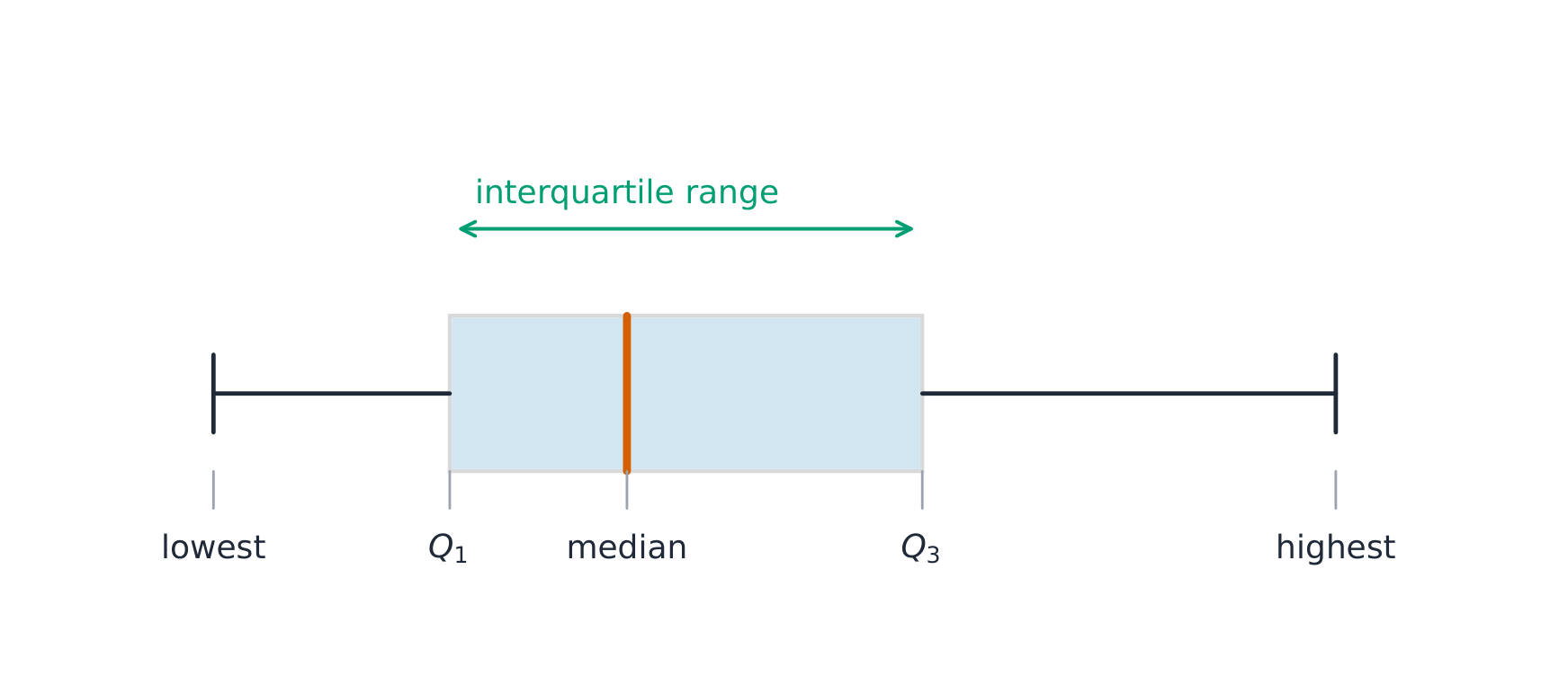
    A boxplot 箱线图 draws the five-number summary: a box from $Q_1$ to $Q_3$ with the median inside, and whiskers to the most extreme non-outlier values. A point is an outlier if it lies more than $1.5\times\text{IQR}$ beyond a quartile – a rule you may be asked to apply. Boxplots are ideal for comparing several groups side by side.

    Worked example. A dataset has $Q_1=20$ and $Q_3=32$, so $\text{IQR}=12$. The outlier fences are $Q_1-1.5(12)=2$ and $Q_3+1.5(12)=50$. Any value below $2$ or above $50$ is flagged as an outlier.

    A box-and-whisker plot shows the quartiles and the range
    A box-and-whisker plot shows the quartiles and the range
    A boxplot draws the five-number summary; the box spans the IQR
    A boxplot draws the five-number summary; the box spans the IQR
    Explore · ⁨חקור⁩

    Explore the five-number summary as a boxplot

    Drag $Q_1$, the median, and $Q_3$ to see the box (its length is the IQR) and how the median's position inside the box reveals skew — a median close to $Q_1$ signals a right-skewed distribution.

    Vocabulary · ⁨מילון מונחים⁩ Train · ⁨אימון⁩
    English עברית
    boxplot/ˈbɒksplɒt/ תרשימת קופסה
    1.9

    Comparing Distributions of a Quantitative Variable

    Syllabus · ⁨סיילבוס⁩
    English

    Enduring Understanding (UNC-1): Graphical representations and statistics allow us to identify and represent key features of data.

    Learning Objective UNC-1.N: Compare graphical representations for multiple sets of quantitative data. [Skill 2.D]

    • UNC-1.N.1 Any of the graphical representations, e.g., histograms, side-by-side boxplots, etc., can be used to compare two or more independent samples on center, variability, clusters, gaps, outliers, and other features.

    Learning Objective UNC-1.O: Compare summary statistics for multiple sets of quantitative data. [Skill 2.D]

    • UNC-1.O.1 Any of the numerical summaries (e.g., mean, standard deviation, relative frequency, etc.) can be used to compare two or more independent samples.
    עברית

    הבנה מתמשכת (UNC-1): ייצוגים גרפיים וסטטיסטיקה מאפשרים לזהות ולייצג תכונות מרכזיות של נתונים.

    מטרות למידה UNC-1.N: להשוות ייצוגים גרפיים עבור מספר קבוצות נתונים כמותיים. [מיומנות 2.D]

    • UNC-1.N.1 כל אחד מהייצוגים הגרפיים, למשל היסטוגרמות, גרפי קופסה בצדדים זה לזה וכו', יכול לשמש להשוואה בין שתי דגימות עצמאיות או יותר בתחומי מרכז, פיזור, אשכולות, רווחים, אנומליות ומאפיינים אחרים.

    מטרות למידה UNC-1.O: להשוות סטטיסטיקות סיכום עבור מספר קבוצות נתונים כמותיים. [מיומנות 2.D]

    • UNC-1.O.1 כל אחד מהסיכומים המספריים (למשל ממוצע, סטיית תקן, תדירות יחסית ועוד) יכול לשמש להשוואה בין שתי דגימות עצמאיות או יותר.

    Source: College Board AP Course and Exam Description · ⁨מקור: תיאור הקורס והמבחן של College Board AP⁩

    To compare two or more groups, compare shape, center, and spread, and mention outliers – always with comparative words ("Group A has a higher median than Group B") and in context. Do not just describe each group separately; make the comparison explicit.

    Explore · ⁨חקור⁩

    Compare distributions with box plots

    A box plot draws the five-number summary. Placing two box plots on the same scale compares their centre (median), spread (IQR = box width) and skew at a glance — the fair way to compare groups.

    1.10

    The Normal Distribution

    Syllabus · ⁨סיילבוס⁩
    Enduring UnderstandingLearning ObjectiveEssential Knowledge

    VAR-2
    The normal distribution can be used to represent some population distributions.

    VAR-2.A
    Compare a data distribution to the normal distribution model. [Skill 2.D]

    • VAR-2.A.1 A parameter is a numerical summary of a population.
    • VAR-2.A.2 Some sets of data may be described as approximately normally distributed. A normal curve is mound-shaped and symmetric. The parameters of a normal distribution are the population mean, $\mu$, and the population standard deviation, $\sigma$.
    • VAR-2.A.3 For a normal distribution, approximately 68% of the observations are within 1 standard deviation of the mean, approximately 95% of observations are within 2 standard deviations of the mean, and approximately 99.7% of observations are within 3 standard deviations of the mean. This is called the empirical rule.
    • VAR-2.A.4 Many variables can be modeled by a normal distribution.
      • Illustrative examples for VAR-2.A:
        • Variables that can be modeled by a normal distribution:
          • Body temperature
          • Weight of a loaf of bread

    VAR-2.B
    Determine proportions and percentiles from a normal distribution. [Skill 3.A]

    • VAR-2.B.1 A standardized score for a particular data value is calculated as (data value − mean)/(standard deviation), and measures the number of standard deviations a data value falls above or below the mean.
    • VAR-2.B.2 One example of a standardized score is a $z$-score, which is calculated as $z\text{-score} = \left(\dfrac{x_i - \mu}{\sigma}\right)$. A $z$-score measures how many standard deviations a data value is from the mean.
    • VAR-2.B.3 Technology, such as a calculator, a standard normal table, or computer-generated output, can be used to find the proportion of data values located on a given interval of a normally distributed random variable.
    • VAR-2.B.4 Given the area of a region under the graph of the normal distribution curve, it is possible to use technology, such as a calculator, a standard normal table, or computer-generated output, to estimate parameters for some populations.

    VAR-2.C
    Compare measures of relative position in data sets. [Skill 2.D]

    • VAR-2.C.1 Percentiles and $z$-scores may be used to compare relative positions of points within a data set or between data sets.

    Source: College Board AP Course and Exam Description · ⁨מקור: תיאור הקורס והמבחן של College Board AP⁩

    A normal distribution 正态分布 is a symmetric, bell-shaped model described by its mean $\mu$ and standard deviation $\sigma$. The empirical rule 经验法则 (68–95–99.7): about 68% of values lie within $1\sigma$ of the mean, 95% within $2\sigma$, and 99.7% within $3\sigma$.

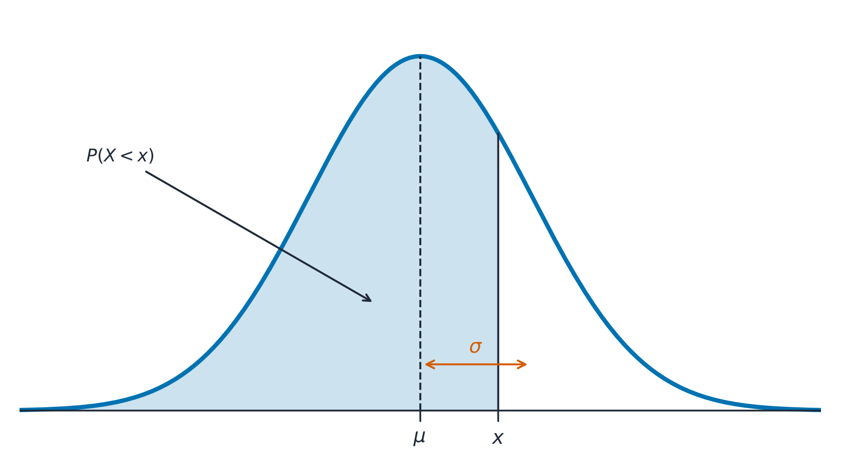
    The normal curve: a probability is the area under it, centred on the mean
    The normal curve: a probability is the area under it, centred on the mean

    A $z$-score 标准分数 measures how many standard deviations a value is from the mean:

    $$z=\frac{x-\mu}{\sigma}.$$
    Convert to a $z$-score, then use the normal table or technology to find the proportion (area) below, above, or between values – and reverse the process to find a value from a given percentile.

    Worked example. Test scores are normal with $\mu=500$ and $\sigma=100$. A score of $700$ has $z=\dfrac{700-500}{100}=2$. By the empirical rule, $95\%$ of scores lie within $2\sigma$, so $2.5\%$ lie above $700$ – meaning a $700$ is at about the $97.5$th percentile.

    The normal curve and the 68-95-99.7 empirical rule
    The normal curve and the 68-95-99.7 empirical rule
    Explore · ⁨חקור⁩

    Explore area under the normal curve

    The proportion of data below a value equals the area under the curve to its left. Shade a tail or a central band to see the 68–95–99.7 empirical rule and read a $z$-score as an area.

    Vocabulary · ⁨מילון מונחים⁩ Train · ⁨אימון⁩
    English עברית
    normal distribution/ˈnɔːml ˌdɪstrɪˈbjuːʃn/ התפלגות נורמלית
    empirical rule/emˈpɪrɪkl ruːl/ כלל ניסויי
    $z$-score/ˈzed skɔː/ מבחן $z$-סקור
    1.10

    Exam tips

    • Describe a distribution by shape, center, spread, and outliers (SOCS) — always in context.
    • The mean is pulled by outliers; the median resists them, so prefer the median for skewed data.
    • For a normal distribution use the 68–95–99.7 rule and z-scores $z=\tfrac{x-\mu}{\sigma}$.
    • Compare distributions with side-by-side boxplots and comment on center, spread, and shape.
    • Standard deviation measures a typical distance from the mean; the IQR pairs with the median.
  • 2

    Exploring Two-Variable Data · ⁨חקר נתוני שני משתנים⁩

    Watch lesson · ⁨צפה בשיעור⁩
    2.1

    Are Two Variables Related? · ⁨האם שני משתנים קשורים?⁩

    Syllabus · ⁨סיילבוס⁩
    English

    Enduring Understanding (VAR-1): Given that variation may be random or not, conclusions are uncertain.

    Learning Objective VAR-1.D: Identify questions to be answered about possible relationships in data. [Skill 1.A]

    • VAR-1.D.1 Apparent patterns and associations in data may be random or not.
    עברית

    הבנה מתמשכת (VAR-1): בשל כך ששינוי עשוי להיות אקראי או לא, המסקנות הן לא וודאות.

    מטרות למידה VAR-1.D: לזהות שאלות יש לענות על קשרים אפשריים בנתונים. [מיומנות 1.A]

    • VAR-1.D.1 דפוסים וקשרים נראים בנתונים עשויים להיות מקריים או לא.

    Source: College Board AP Course and Exam Description · ⁨מקור: תיאור הקורס והמבחן של College Board AP⁩

    English

    Two-variable data let us ask whether two characteristics are associated 关联 – whether knowing one tells you something about the other. An explanatory variable 解释变量 (the "input") may help predict a response variable 响应变量 (the "output"). Association is not the same as causation.

    עברית

    נתונים דו-משתניים מאפשרים לשאול האם שתי מאפיינים קשורים – האם ידע אחד מספק מידע על השני. משתנה הסבר (ה"קלט") עשוי לסייע בחיזוי משתנה תגובה (ה"יציאה"). קשר אינו זהה לחיבור סיבתי.

    2.2

    Two Categorical Variables · ⁨שני משתנים קטגוריאליים⁩

    Syllabus · ⁨סיילבוס⁩
    English

    Enduring Understanding (UNC-1): Graphical representations and statistics allow us to identify and represent key features of data.

    Learning Objective UNC-1.P: Compare numerical and graphical representations for two categorical variables. [Skill 2.D]

    • UNC-1.P.1 Side-by-side bar graphs, segmented bar graphs, and mosaic plots are examples of bar graphs for one categorical variable, broken down by categories of another categorical variable.
    • UNC-1.P.2 Graphical representations of two categorical variables can be used to compare distributions and/or determine if variables are associated.
    • UNC-1.P.3 A two-way table, also called a contingency table, is used to summarize two categorical variables. The entries in the cells can be frequency counts or relative frequencies.
    • UNC-1.P.4 A joint relative frequency is a cell frequency divided by the total for the entire table.
    עברית

    הבנה מתמשכת (UNC-1): ייצוגים גרפיים וסטטיסטיקה מאפשרים לזהות ולייצג תכונות מרכזיות של נתונים.

    מטרות למידה UNC-1.P: להשוות ייצוגים מספריים וגרפיים לשני משתנים קטגוריאליים. [מיומנות 2.D]

    • UNC-1.P.1 גרפי עמודות בצדדים זה לזה, גרפי עמודות מחולקים (segmented bar graphs) ותמונות מוזאיק הם דוגמאות לגרפי עמודות למשתנה קטגוריאלי אחד, המפורקים לפי קטגוריות של משתנה קטגוריאלי אחר.
    • UNC-1.P.2 ייצוגים גרפיים של שני משתנים קטגוריאליים יכולים לשמש להשוואת התפלגויות ו/או לקבוע האם משתנים קשורים.
    • UNC-1.P.3 טבלה דו-כיוונית, הנקראת גם טבלת תלות, משמשת לסיכום שני משתנים קטגוריאליים. הכניסות בתאים יכולות להיות ספירות תדירות או תדירויות יחסיות.
    • UNC-1.P.4 תדירות יחסית משותפת היא תדירות תא המחולקת בסך הכל של הטבלה כולה.

    Source: College Board AP Course and Exam Description · ⁨מקור: תיאור הקורס והמבחן של College Board AP⁩

    English

    A two-way table 双向表 (contingency table) counts individuals by two categorical variables at once. A marginal distribution 边缘分布 is a row or column total written as a fraction of the grand total (the totals themselves are just counts). Comparing the inside cells shows whether the variables are related.

    עברית

    טבלה דו-כיוונית (טבלת תלות) סופרת פרטים לפי שני משתנים קטגוריאליים בו-זמנית. התפלגות שוליים היא סכום שורה או עמודה המוצג כשבר מהסך הכללי (הסכומים עצמם הם פשוט ספירות). השוואת התאים הפנימיים מראה האם המשתנים קשורים.

    2.3

    Comparing Groups with Conditional Distributions · ⁨השוואת קבוצות באמצעות התפלגויות תנאי⁩

    Syllabus · ⁨סיילבוס⁩
    English

    Enduring Understanding (UNC-1): Graphical representations and statistics allow us to identify and represent key features of data.

    Learning Objective UNC-1.Q: Calculate statistics for two categorical variables. [Skill 2.C]

    • UNC-1.Q.1 The marginal relative frequencies are the row and column totals in a two-way table divided by the total for the entire table.
    • UNC-1.Q.2 A conditional relative frequency is a relative frequency for a specific part of the contingency table (e.g., cell frequencies in a row divided by the total for that row).

    Learning Objective UNC-1.R: Compare statistics for two categorical variables. [Skill 2.D]

    • UNC-1.R.1 Summary statistics for two categorical variables can be used to compare distributions and/or determine if variables are associated.
    עברית

    הבנה מתמשכת (UNC-1): ייצוגים גרפיים וסטטיסטיקה מאפשרים לזהות ולייצג תכונות מרכזיות של נתונים.

    מטרות למידה UNC-1.Q: לחשב סטטיסטיקות לשני משתנים קטגוריאליים. [מיומנות 2.C]

    • UNC-1.Q.1 התדירויות היחסיות השוליות הן סכומי שורות ועמודות בטבלה דו-צירית מחולקים בסך הכל של הטבלה כולה.
    • UNC-1.Q.2 תדירות יחסית מותנית היא תדירות יחסית עבור חלק ספציפי בטבלת העלילה (למשל, תדירויות תאים בשורה מחולפות בסך הכל של אותה שורה).

    מטרת למידה UNC-1.R: השוואת סטטיסטיקה לשני משתנים קטגוריאליים. [Skill 2.D]

    • UNC-1.R.1 סטטיסטיקת סיכום לשני משתנים קטגוריאליים יכולה לשמש להשוואת ההתפלגויות ו/או לקבוע האם המשתנים קשורים זה לזה.

    Source: College Board AP Course and Exam Description · ⁨מקור: תיאור הקורס והמבחן של College Board AP⁩

    English

    A conditional distribution 条件分布 is the distribution of one variable within a fixed category of the other (found by dividing each cell by its row or column total). If the conditional distributions differ across groups, the two variables are associated; if they are the same, there is no association. Segmented bar charts 分段条形图 or mosaic plots display them.

    עברית

    התפלגות תנאית היא ההתפלגות של משתנה אחד בתוך קטגוריה קבועה של המשתנה השני (נמצאת על ידי חלוקת כל תא בסכום השורה או העמודה שלו). אם ההתפלגויות התנאיות שונות בין קבוצות, שני המשתנים קשורים; אם הן זהות, אין קשר. גרפי עמודות מקוטעים או גרפי פיסות מציגים אותן.

    2.4

    Scatterplots for Two Quantitative Variables · ⁨גרפי פיזור לשני משתנים כמותיים⁩

    Syllabus · ⁨סיילבוס⁩
    English

    Enduring Understanding (UNC-1): Graphical representations and statistics allow us to identify and represent key features of data.

    Learning Objective UNC-1.S: Represent bivariate quantitative data using scatterplots. [Skill 2.B]

    • UNC-1.S.1 A bivariate quantitative data set consists of observations of two different quantitative variables made on individuals in a sample or population.
    • UNC-1.S.2 A scatterplot shows two numeric values for each observation, one corresponding to the value on the $x$-axis and one corresponding to the value on the $y$-axis.
    • UNC-1.S.3 An explanatory variable is a variable whose values are used to explain or predict corresponding values for the response variable.

    Enduring Understanding (DAT-1): Regression models may allow us to predict responses to changes in an explanatory variable.

    Learning Objective DAT-1.A: Describe the characteristics of a scatter plot. [Skill 2.A]

    • DAT-1.A.1 A description of a scatter plot includes form, direction, strength, and unusual features.
    • DAT-1.A.2 The direction of the association shown in a scatterplot, if any, can be described as positive or negative.
    • DAT-1.A.3 A positive association means that as values of one variable increase, the values of the other variable tend to increase. A negative association means that as values of one variable increase, values of the other variable tend to decrease.
    • DAT-1.A.4 The form of the association shown in a scatterplot, if any, can be described as linear or non-linear to varying degrees.
    • DAT-1.A.5 The strength of the association is how closely the individual points follow a specific pattern, e.g., linear, and can be shown in a scatterplot. Strength can be described as strong, moderate, or weak.
    • DAT-1.A.6 Unusual features of a scatter plot include clusters of points or points with relatively large discrepancies between the value of the response variable and a predicted value for the response variable.
    עברית

    הבנה מתמשכת (UNC-1): ייצוגים גרפיים וסטטיסטיקה מאפשרים לזהות ולייצג תכונות מרכזיות של נתונים.

    מטרת למידה UNC-1.S: נייגון נתונים כמותיים בי-משתניים באמצעות גרפי פיזור. [Skill 2.B]

    • UNC-1.S.1 ערכת נתונים כמותיים בי-משתניים מורכבת מצפייה על שני משתנים כותיים שונים שנערכו על פרטים בדגימה או באוכלוסייה.
    • UNC-1.S.2 גרף פיזור מראה שני ערכים מספריים לכל צפייה, אחד המתאים לערך על ציר ה $x$ ואחד המתאים לערך על ציר ה $y$.
    • UNC-1.S.3 משתנה הסבר הוא משתנה whose ערכיו משמשים להסביר או לחזות ערכים תואמים במשתנה התגובה.

    הבנה מתמשכת (DAT-1): מודלים רגרסיה עשויים לאפשר לנו לחזות תגובות לשינויים במשתנה הסבר.

    מטרת למידה DAT-1.A: לתאר את מאפייני גרף פיזור. [Skill 2.A]

    • DAT-1.A.1 תיאור גרף פיזור כולל צורה, כיוון, חוזק ותכונות בלתי רגילות.
    • DAT-1.A.2 הכיוון של ההקשר המוצג בגרף פיזור, אם קיים, ניתן לתאר כחיובי או שלילי.
    • DAT-1.A.3 הקשר חיובי פירושו שככל שערכי משתנה אחד עולים, ערכי המשתנה השני נוטים לעלות. הקשר שלילי פירושו שככל שערכי משתנה אחד עולים, ערכי המשתנה השני נוטים לרדת.
    • DAT-1.A.4 הצורה של ההקשר המוצג בגרף פיזור, אם קיים, ניתן לתאר כליניארי או לא-ליניארי ברמת התייחסות שונות.
    • DAT-1.A.5 חוזק ההקשר הוא עד כמה הנקודות הבודדות עוקבות אחר דפוס ספציפי, לדוגמה ליניארי, והוא יכול להיות מוצג בגרף פיזור. חוזק יכול להתאפיין בחזק, בינוני או חלש.
    • DAT-1.A.6 תכונות בלתי רגילות בגרף פיזור כוללות אשכולות של נקודות או נקודות עם אי-התאמות גדולות יחסית בין ערך משתנה התגובה לערך החזוי עבור משתנה התגובה.

    Source: College Board AP Course and Exam Description · ⁨מקור: תיאור הקורס והמבחן של College Board AP⁩

    English

    A scatterplot 散点图 plots each individual as a point, explanatory variable on the $x$-axis and response on the $y$-axis. Describe it with DUFS: Direction (positive/negative), Unusual features (outliers, clusters), Form (linear or curved), and Strength (how tightly the points follow the pattern) – always in context.

    עברית

    תרפיס פיזור מצייר כל פרט כנקודה, משתנה הסבר על ציר ה-$x$ ומשתנה התגובה על ציר ה-$y$. מתארים אותו באמצעות DUFS: כיוון (חיובי/שלילי), מאפיינים בלתי רגילים (חריגים, אשכולות), צורה (ליניארית או מעוקלת), וחוזק (כמה הנקודות עוקבות אחרי הדפוס) – תמיד בהקשר.

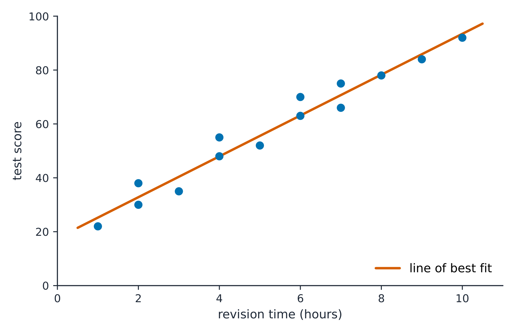
    קו התאמה מיטבית עובר באמצע הנקודות המפוזרות
    קו התאמה מיטבית עובר באמצע הנקודות המפוזרות
    2.5

    Correlation · ⁨קורלציה⁩

    Syllabus · ⁨סיילבוס⁩
    English

    Enduring Understanding (DAT-1): Regression models may allow us to predict responses to changes in an explanatory variable.

    Learning Objective DAT-1.B: Determine the correlation for a linear relationship. [Skill 2.C]

    • DAT-1.B.1 The correlation, $r$, gives the direction and quantifies the strength of the linear association between two quantitative variables.
    • DAT-1.B.2 The correlation coefficient can be calculated by: $r = \dfrac{1}{n-1} \sum \left( \dfrac{x_i - \bar{x}}{s_x} \right) \left( \dfrac{y_i - \bar{y}}{s_y} \right)$. However, the most common way to determine $r$ is by using technology.
    • DAT-1.B.3 A correlation coefficient close to 1 or $-1$ does not necessarily mean that a linear model is appropriate.

    Learning Objective DAT-1.C: Interpret the correlation for a linear relationship. [Skill 4.B]

    • DAT-1.C.1 The correlation, $r$, is unit-free, and always between $-1$ and 1, inclusive. A value of $r = 0$ indicates that there is no linear association. A value of $r = 1$ or $r = -1$ indicates that there is a perfect linear association.
    • DAT-1.C.2 A perceived or real relationship between two variables does not mean that changes in one variable cause changes in the other. That is, correlation does not necessarily imply causation.
    עברית

    הבנה מתמשכת (DAT-1): מודלים רגרסיה עשויים לאפשר לנו לחזות תגובות לשינויים במשתנה הסבר.

    מטרת למידה DAT-1.B: לקבוע את הקורלציה לקשר ליניארי. [Skill 2.C]

    • DAT-1.B.1 המקדם, $r$, מספק את הכיוון ומכמת את חוזק ההקשר הליניארי בין שני משתנים כותיים.
    • DAT-1.B.2 מקדם המתאם ניתן לחישוב על ידי: $r = \dfrac{1}{n-1} \sum \left( \dfrac{x_i - \bar{x}}{s_x} \right) \left( \dfrac{y_i - \bar{y}}{s_y} \right)$. עם זאת, הדרך הנפוצה ביותר לקבוע $r$ היא באמצעות שימוש בטכנולוגיה.
    • DAT-1.B.3 מקדם מתאם הקרוב ל-1 או ל$-1$ אינו בהכרח מצביע על כך שדגם ליניארי הוא מתאים.

    מטרת למידה DAT-1.C: פרשן את המקדם במתאם ליניארי. [מיומנות 4.B]

    • DAT-1.C.1 המקדם, $r$, חסר יחידות, תמיד נמצא בין $-1$ ל-1, כולל קצוות. ערך של $r = 0$ מעיד על כך שאין מתאם ליניארי. ערך של $r = 1$ או $r = -1$ מעיד על כך שקיים מתאם ליניארי מושלם.
    • DAT-1.C.2 קשר נתפס או אמיתי בין משתנים שניים אינו אומר שהשינויים במשתנה אחד גורמים לשינויים במשתנה השני. כלומר, מתאם אינו implies בהכרח סיבתיות.

    Source: College Board AP Course and Exam Description · ⁨מקור: תיאור הקורס והמבחן של College Board AP⁩

    English
    What r actually measures

    The correlation coefficient 相关系数 $r$ measures the strength and direction of a linear relationship. It runs from $-1$ to $1$: near $\pm 1$ is strong linear, near $0$ is weak linear. $r$ has no units and does not change if you swap the variables. Warnings: $r$ only measures linear strength, it is not resistant to outliers, and a strong $r$ does not prove causation.

    עברית
    מה r מודד בפועל

    המקדם הקורלציה $r$ מדד את חוזק וכיוון הקשר הליניארי. הוא נע בין $-1$ ל$1$: קרוב ל$\pm 1$ הוא ליניארי חזק, וקרוב ל$0$ הוא ליניארי חלש. $r$ אין לו יחידות מידה ואינו משתנה אם מחליפים את המשתנים. אזהרות: $r$ מדד רק חוזק ליניארי, הוא אינו עמיד בפני ערכים קיצוניים, וחוזק גבוה ב$r$ לא מוכיח סיבתיות.

    קורלציה חיובית עולה יחד; קורלציה שלילית זזה בכיוונים הפוכים
    קורלציה חיובית עולה יחד; קורלציה שלילית זזה בכיוונים הפוכים
    Explore · ⁨חקור⁩

    Strength of a linear relationship · ⁨חוזק הקשר הליניארי⁩

    Correlation $r$ runs from $-1$ to $1$: near $\pm1$ the points hug a line, near 0 they scatter. Change it and watch the cloud tighten or spread. · ⁨קורלציה $r$ נעה בין $-1$ ל$1$: קרוב ל$\pm1$ הנקודות צמודות לקו, קרוב ל-0 הן מפוזרות. שנה אותו והרה את הענן מתכווץ או מתפשט.⁩

    2.6

    Linear Regression Models · ⁨דגמי רגרסיה ליניארית⁩

    Syllabus · ⁨סיילבוס⁩
    Enduring UnderstandingLearning ObjectiveEssential Knowledge

    DAT-1
    Regression models may allow us to predict responses to changes in an explanatory variable.

    DAT-1.D
    Calculate a predicted response value using a linear regression model. [Skill 2.C]

    • DAT-1.D.1 A simple linear regression model is an equation that uses an explanatory variable, $x$, to predict the response variable, $y$.
    • DAT-1.D.2 The predicted response value, denoted by $\hat{y}$, is calculated as $\hat{y} = a + bx$, where $a$ is the $y$-intercept and $b$ is the slope of the regression line, and $x$ is the value of the explanatory variable.
    • DAT-1.D.3 Extrapolation is predicting a response value using a value for the explanatory variable that is beyond the interval of $x$-values used to determine the regression line. The predicted value is less reliable as an estimate the further we extrapolate.

    Source: College Board AP Course and Exam Description · ⁨מקור: תיאור הקורס והמבחן של College Board AP⁩

    English

    The least-squares regression line 最小二乘回归线 predicts the response: $\hat{y}=a+bx$, where $\hat{y}$ is the predicted response. The slope 斜率 $b$ is the predicted change in $y$ per one-unit increase in $x$; the $y$-intercept 截距 $a$ is the predicted $y$ when $x=0$. Interpret both in context and with units – a graded skill. Avoid extrapolation 外推 (predicting far outside the data).

    Worked example. A study of hours studied ($x$) and test score ($y$) gives $\hat{y}=20+3x$. The slope means each extra hour of study is associated with a predicted $3$-point increase. A student who studies $5$ hours is predicted to score $\hat{y}=20+3(5)=35$.

    עברית

    קו הרגרסיה לפחות-הריבועים מנבא את התגובה: $\hat{y}=a+bx$, כאשר $\hat{y}$ היא התגובה המוכחת. שיפוע $b$ הוא השינוי המוכחת ב$y$ לכל עלייה של יחידה אחת ב$x$; ה$y$-חתך $a$ הוא ה$y$ המוכחת כשה$x=0$. יש לפרש שניהם בהקשר ובכלליות עם יחידות מידה – מיומנות מוערכת. יש להימנע מאקסטרפולציה (הכרת תחזית הרחוקה מאוד מהנתונים).

    דוגמה מופרדת. מחקר על שעות לימוד ($x$) ותוצאת מבחן ($y$) נתנו $\hat{y}=20+3x$. השיפוע אומר שכל שעת לימוד נוספת קשורה לעלייה מוכחת של $3$ נקודות. סטודנט שלימד $5$ שעות מוכתב שתציין $\hat{y}=20+3(5)=35$.

    Explore · ⁨חקור⁩

    Fit a least-squares line · ⁨התאמת קו פחות-הריבועים⁩

    A regression line is the best straight-line fit, minimising the squared vertical distances. Its slope predicts how $y$ changes per unit of $x$. · ⁨קו רגרסיה הוא ההתאמה הישרה הטובה ביותר, המזערת את הריבועים של המרחקים האנכיים. שיפועו מתنبא כיצד $y$ משתנה ליחידה אחת של $x$.⁩

    2.7

    Residuals · ⁨שאריות⁩

    Syllabus · ⁨סיילבוס⁩
    English

    Enduring Understanding (DAT-1): Regression models may allow us to predict responses to changes in an explanatory variable.

    Learning Objective DAT-1.E: Represent differences between measured and predicted responses using residual plots. [Skill 2.B]

    • DAT-1.E.1 The residual is the difference between the actual value and the predicted value: $\text{residual} = y - \hat{y}$.
    • DAT-1.E.2 A residual plot is a plot of residuals versus explanatory variable values or predicted response values.

    Learning Objective DAT-1.F: Describe the form of association of bivariate data using residual plots. [Skill 2.A]

    • DAT-1.F.1 Apparent randomness in a residual plot for a linear model is evidence of a linear form to the association between the variables.
    • DAT-1.F.2 Residual plots can be used to investigate the appropriateness of a selected model.
    עברית

    הבנה מתמשכת (DAT-1): מודלים רגרסיה עשויים לאפשר לנו לחזות תגובות לשינויים במשתנה הסבר.

    מטרת למידה DAT-1.E: נציג הבדלים בין תגובות נמדדות לתגובות צפויות באמצעות גרפי שאריות. [מיומנות 2.B]

    • DAT-1.E.1 השארית היא ההפרש בין הערך בפועל לערך הצפוי: $\text{residual} = y - \hat{y}$.
    • DAT-1.E.2 גרף שאריות הוא גרף של שאריות נגד ערכי משתנה ההסבר או ערכי התגובה הצפויים.

    מטרת למידה DAT-1.F: תאר את צורת המתאם של נתונים דו-משתנים באמצעות גרפי שאריות. [מיומנות 2.A]

    • DAT-1.F.1 אקראיות apparent בגרף שאריות לדגם ליניארי היא עדות לצורה ליניארית במתאם בין המשתנים.
    • DAT-1.F.2 גרפי שאריות יכולים לשמש לבדיקת ההתאמה של דגם שנבחר.

    Source: College Board AP Course and Exam Description · ⁨מקור: תיאור הקורס והמבחן של College Board AP⁩

    English
    Least-squares regression

    A residual 残差 is actual minus predicted, $y-\hat{y}$: how far a point sits above (+) or below (−) the line. A residual plot 残差图 graphs residuals against $x$. If it shows no pattern (random scatter), a linear model is appropriate; a curved or fanning pattern means the linear model is a poor fit.

    Worked example. Continuing the study above, a student who studied $5$ hours actually scored $40$. The residual is $y-\hat{y}=40-35=+5$: the line under-predicted by $5$ points, so this point sits above the line.

    עברית
    רגרסיה פחותים מרבעים

    שארית היא האמת פחות הכרעה, $y-\hat{y}$: כמה נקודה נמצאת מעל (+) או מתחת (−) לקו. גרף שאריות מצייר שאריות מול $x$. אם הוא מראה אין דפוס (פיזור אקראי), דגם ליניארי מתאים; דפוס מעוגל או מתפשט מסמן שהדגם הליניארי הוא התאמה גרועה.

    דוגמה מופרדת. בהמשך למחקר לעיל, סטודנט שלימד $5$ שעות ציין בפועל $40$. השארית היא $y-\hat{y}=40-35=+5$: הקו הכרה נמוכה ב$5$ נקודות, ולכן הנקודה הזו נמצאת מעל הקו.

    ארבעה מאגרים נתונים עם r זהה וקו רגרסיה זהה אך ארבעה צורות שונות
    אזהרה לגבי ⟨$r$⟩ והקו: כל ארבעת מאגרי הנתונים הם אותו ⟨$r=0.82$⟩ ואותו ⟨$\hat{y}=3.0+0.5x$⟩, אך רק הראשון הוא ליניארי אמיתי. הגרפים מפוזרים קשה להבחין ביניהם — גרף השאריות בתחתית כל אחד הוא מה חושף את העיקום, הערך הקיצוני ונקודת ההשפעה הגבוהה.
    2.8

    Least-Squares Regression and Its Fit · ⁨רגרסיה לפחות-הריבועים והתאמתה⁩

    Syllabus · ⁨סיילבוס⁩
    English

    Enduring Understanding (DAT-1): Regression models may allow us to predict responses to changes in an explanatory variable.

    Learning Objective DAT-1.G: Estimate parameters for the least-squares regression line model. [Skill 2.C]

    • DAT-1.G.1 The least-squares regression model minimizes the sum of the squares of the residuals and contains the point $(\bar{x}, \bar{y})$.
    • DAT-1.G.2 The slope, $b$, of the regression line can be calculated as $b = r \left( \dfrac{s_y}{s_x} \right)$ where $r$ is the correlation between $x$ and $y$, $s_y$ is the sample standard deviation of the response variable, $y$, and $s_x$ is the sample standard deviation of the explanatory variable, $x$.
    • DAT-1.G.3 Sometimes, the $y$-intercept of the line does not have a logical interpretation in context.
    • DAT-1.G.4 In simple linear regression, $r^2$ is the square of the correlation, $r$. It is also called the coefficient of determination. $r^2$ is the proportion of variation in the response variable that is explained by the explanatory variable in the model.

    Learning Objective DAT-1.H: Interpret coefficients for the least-squares regression line model. [Skill 4.B]

    • DAT-1.H.1 The coefficients of the least-squares regression model are the estimated slope and $y$-intercept.
    • DAT-1.H.2 The slope is the amount that the predicted $y$-value changes for every unit increase in $x$.
    • DAT-1.H.3 The $y$-intercept value is the predicted value of the response variable when the explanatory variable is equal to $0$. The formula for the $y$-intercept, $a$, is $a = \bar{y} - b\bar{x}$.
    עברית

    הבנה מתמשכת (DAT-1): מודלים רגרסיה עשויים לאפשר לנו לחזות תגובות לשינויים במשתנה הסבר.

    מטרת למידה DAT-1.G: העריך פרמטרים עבור דגם קו הרגרסיה של סכומי רבועים מינימליים. [מיומנות 2.C]

    • DAT-1.G.1 דגם הרגרסיה של סכומי רבועים מינימליים ממזער את סכום רבועות השאריות ומכיל את הנקודה $(\bar{x}, \bar{y})$.
    • DAT-1.G.2 השיפוע, $b$, של קו הרגרסיה ניתן לחישוב כ $b = r \left( \dfrac{s_y}{s_x} \right)$ כאשר $r$ הוא הקורלציה בין $x$ ל $y$, $s_y$ היא סטיית התקן המדגמית של משתנה התגובה, $y$, ו $s_x$ היא סטיית התקן המדגמית של משתנה ההסבר, $x$.
    • DAT-1.G.3 לעיתים, החיתוך עם ציר ה $y$ של הקו אינו בעל פרשנות לוגית בהקשר נתון.
    • DAT-1.G.4 ברגרסיה ליניארית פשוטה, $r^2$ הוא ריבוע הקורלציה, $r$. הוא מכונה גם מקדם הקביעה. $r^2$ הוא היחס שבהתאם אליו השונות במשתנה התגובה מוסברת על ידי משתנה ההסבר במודל.

    מטרת למידה DAT-1.H: פרש מקדמים במודל קו הרגרסיה לפחות ריבועים. [מיומנות 4.B]

    • DAT-1.H.1 המקדמים במודל הרגרסיה לפחות ריבועים הם השיפוע המוערך וחיתוך ציר ה $y$.
    • DAT-1.H.2 השיפוע הוא הכמות שבה ישתנה הערך המוצף של $y$ עבור כל עלייה של יחידה אחת ב $x$.
    • DAT-1.H.3 ערך חיתוך ציר ה $y$ הוא הערך המוצף של משתנה התגובה כאשר משתנה ההסבר שווה ל $0$. הנוסחה לחיתוך ציר ה $y$, $a$, היא $a = \bar{y} - b\bar{x}$.

    Source: College Board AP Course and Exam Description · ⁨מקור: תיאור הקורס והמבחן של College Board AP⁩

    English

    The line minimizes the sum of squared residuals. Its fit is measured by:

    • $s$, the standard deviation of the residuals – the typical prediction error, in the response's units.
    • $r^2$, the coefficient of determination 决定系数 – the proportion of the variation in $y$ that the linear model explains (a value between $0$ and $1$; multiply by $100$ to state it as a percent). Report it in context: "$r^2 = 0.81$ means 81% of the variation in $y$ is explained by the linear relationship with $x$."
    עברית
    הקו לפחות-הריבועים ממזער את סכום השאריות המרובעות
    הקו לפחות-הריבועים ממזער את סכום השאריות המרובעות

    הקו ממזער את סכום השאריות המרובעות. ההתאמה שלו נמדדת על ידי:

    • ⟨$s$⟩, סטיית התקן של השאריות – טעות הכרעה טיפוסית, ביחידות התגובה.
    • $r^2$, מקדם הקביעה – החלק מהשינוי ב$y$ שהמודל הליניארי מסביר (ערך בין $0$ ל$1$; כפול ב-$100$ כדי לבטאו באחוזים). דווח במרחב: "$r^2 = 0.81$ פירושו ש-81% מהשינוי ב$y$ מוסבר על ידי הקשר הליניארי עם $x$."
    Vocabulary · ⁨מילון מונחים⁩ Train · ⁨אימון⁩
    English עברית
    associated/əˈsəʊsɪeɪtɪd/ קשור
    explanatory variable/ekˈsplænətəri ˈveərɪəbl/ משתנה הסבר
    response variable/rɪˈspɒns ˈveərɪəbl/ משתנה תגובה
    two-way table/tuː weɪ ˈteɪbl/ טבלה דו-כיוונית
    marginal distributions/ˈmɑːdʒɪnl ˌdɪstrɪˈbjuːʃnz/ התפלגויות שוליים
    conditional distribution/kənˈdɪʃənl ˌdɪstrɪˈbjuːʃn/ התפלגות תנאיית
    Segmented bar charts/seɡˈmentɪd bɑː tʃɑːts/ גרפי עמודות מחולקים
    scatterplot/ˈskætəplɒt/ תרשים פיזור
    correlation coefficient/ˌkɒrɪˈleɪʃn ˌkəʊɪˈfɪʃənt/ מקדם קורלציה
    least-squares regression line/liːst skweəz rɪˈɡreʃn laɪn/ ישר רגרסיה של פחותים מרובעים
    slope/sləʊp/ שיפוע
    y-intercept/waɪ ˌɪntəˈsept/ נקודת חיתוך עם ציר ה-y
    extrapolation/ekˈstræpəleɪʃn/ אקסטרפולציה
    residual/rɪˈsɪdʒuːəl/ שארית
    residual plot/rɪˈsɪdʒuːəl plɒt/ גרף שאריות
    coefficient of determination/ˌkəʊɪˈfɪʃənt ɒv dɪˌtɜːmɪˈneɪʃn/ מקדם הקביעה
    high-leverage/haɪ ˈliːvərɪdʒ/ בעל השפעה גבוהה
    influential/ˌɪnfluːˈenʃl/ משפיע
    2.9

    Departures from Linearity · ⁨סטייה מליניאריות⁩

    Syllabus · ⁨סיילבוס⁩
    English

    Enduring Understanding (DAT-1): Regression models may allow us to predict responses to changes in an explanatory variable.

    Learning Objective DAT-1.I: Identify influential points in regression. [Skill 2.A]

    • DAT-1.I.1 An outlier in regression is a point that does not follow the general trend shown in the rest of the data and has a large residual when the Least Squares Regression Line (LSRL) is calculated.
    • DAT-1.I.2 A high-leverage point in regression has a substantially larger or smaller $x$-value than the other observations have.
    • DAT-1.I.3 An influential point in regression is any point that, if removed, changes the relationship substantially. Examples include much different slope, $y$-intercept, and/or correlation. Outliers and high leverage points are often influential.

    Learning Objective DAT-1.J: Calculate a predicted response using a least-squares regression line for a transformed data set. [Skill 2.C]

    • DAT-1.J.1 Transformations of variables, such as evaluating the natural logarithm of each value of the response variable or squaring each value of the explanatory variable, can be used to create transformed data sets, which may be more linear in form than the untransformed data.
    • DAT-1.J.2 Increased randomness in residual plots after transformation of data and/or movement of $r^2$ to a value closer to 1 offers evidence that the least-squares regression line for the transformed data is a more appropriate model to use to predict responses to the explanatory variable than the regression line for the untransformed data.
    עברית

    הבנה מתמשכת (DAT-1): מודלים רגרסיה עשויים לאפשר לנו לחזות תגובות לשינויים במשתנה הסבר.

    מטרת למידה DAT-1.I: זיהוי נקודות השפעתיות ברגרסיה. [מיומנות 2.A]

    • DAT-1.I.1 נקודת חריגה ברגרסיה היא נקודה שלא עוקבת אחר מגמה כללית המוצגת בשאר הנתונים ולها שארית גדולה כאשר מחושב קו הרגרסיה לפחות ריבועים (LSRL).
    • DAT-1.I.2 נקודת שילוב גבוהה ברגרסיה היא נקודה שערכה ב $x$ גדול או קטן משמעותית מערכיה של שאר התצפיות.
    • DAT-1.I.3 נקודה השפעתית ברגרסיה היא כל נקודה שהסרתה משנה את הקשר באופן משמעותי. דוגמאות כוללות שיפוע שונה מאוד, חיתוך ציר ה $y$ ו/או קורלציה שונים. נקודות חריגה ונקודות שילוב גבוהות הן לעיתים נקודות השפעתיות.

    מטרת למידה DAT-1.J: לחשב תגובה מוצפת באמצעות קו רגרסיה לפחות ריבועים עבור קבץ נתונים מופעל. [מיומנות 2.C]

    • DAT-1.J.1 הפעלות של משתנים, כמו חישוב הלוגריתם הטבעי של כל ערך במשתנה התגובה או הריבוע של כל ערך במשתנה ההסבר, יכולות לשמש ליצירת קבצי נתונים מופעלים, שעשויים להיות יותר ליניאריים בצורתם מאשר הנתונים לא מופעלים.
    • DAT-1.J.2 הגדלת האקראיות בגרפי שאריות לאחר הפעלת נתונים ו/או תנועת $r^2$ לערך הקרוב יותר ל-1 מספקת ראיה לכך שקו הרגרסיה לפחות ריבועים עבור הנתונים המופעלים הוא מודל מתאים יותר לשימוש כדי לחזות תגובות למשתנה ההסבר מאשר קו הרגרסיה עבור הנתונים לא מופעלים.

    Source: College Board AP Course and Exam Description · ⁨מקור: תיאור הקורס והמבחן של College Board AP⁩

    English

    Some points strongly affect the line. A high-leverage 高杠杆 point has an extreme $x$-value; an influential 有影响的 point noticeably changes the slope or $r$ when removed; an outlier here is a point with a large residual. When the pattern is curved, transform a variable (e.g. take a log) to straighten it, then fit a line to the transformed data.

    עברית

    חלק מהנקודות משפיעות חזק על הקו. נקודה בעלת שקל גבוה היא בעלת ערך קיצוני ב$x$; נקודה משפיעה משנה משמעותית את השיפוע או את ה$r$ כאשר נשלפת; נקודת אנומליה כאן היא נקודה עם שארית גדולה. כאשר הדפוס מעוקם, עבור משתנה (למשל, לקחת לוגaritmo) כדי להחליק אותו, ולאחר מכן התאם ישר לנתונים המעובים.

    2.9

    Exam tips · ⁨טיפים לבחינות⁩

    English
    • On a scatterplot describe direction, form, strength, and outliers; $r$ ranges $-1$ to $1$.
    • Correlation is not causation — a lurking variable can drive both.
    • Interpret the slope of the least-squares line in context ("per one unit of $x$, predicted $y$ changes by $b$").
    • Check a residual plot: no pattern means a line fits; a curve means it does not. Avoid extrapolation.
    • $r^2$ is the fraction of variation in $y$ explained by the model.
    עברית
    • בגרף פיזור תאר כיוון, צורה, חוזקה ואנומליות; $r$ נע בין $-1$ ל$1$.
    • קורלציה אינה סיבתיות – משתנה נסתר עשוי להיות הגורם בשניהם.
    • פרש את השיפוע של הישר פחות הריבועים במרחב ("כל שינוי של יחידה אחת ב$x$, השינוי הנבוא ב$y$ הוא $b$")."
    • בדוק גרף שאריות: העדר דפוס מצביע על התאמה טובה לישר; עיקום מצביע שלא. הימנע מהתנבאות מחוץ לטווח.
    • $r^2$ הוא השבר של השינוי ב$y$ שמוסבר על ידי המודל.
  • 3

    Collecting Data · ⁨איסוף נתונים⁩

    Watch lesson · ⁨צפה בשיעור⁩
    3.1

    Can We Trust the Data We Collected? · ⁨האם ניתן לסמוך על הנתונים שאספנו?⁩

    Syllabus · ⁨סיילבוס⁩
    English

    Enduring Understanding (VAR-1): Given that variation may be random or not, conclusions are uncertain.

    Learning Objective VAR-1.E: Identify questions to be answered about data collection methods. [Skill 1.A]

    • VAR-1.E.1 Methods for data collection that do not rely on chance result in untrustworthy conclusions.
    עברית

    הבנה מתמשכת (VAR-1): בשל כך ששינוי עשוי להיות אקראי או לא, המסקנות הן לא וודאות.

    מטרת למידה VAR-1.E: זיהוי שאלות להשקפה על שיטות איסוף נתונים. [מיומנות 1.A]

    • VAR-1.E.1 שיטות לאיסוף נתונים שאינן מבוססות על chance מובילות למסקנות שאינן אמינות.

    Source: College Board AP Course and Exam Description · ⁨מקור: תיאור הקורס והמבחן של College Board AP⁩

    English

    A conclusion is only as good as the data behind it. How data are collected decides what you may conclude – whether you can generalize to a population 总体, and whether you can claim cause and effect. Poorly collected data can be worse than none.

    עברית

    המסקנה טובה רק בהתאם לנתונים העומדים מאחוריה. איך הנתונים אספו קובע מה ניתן להסיק – האם ניתן לגנרליזציה לאוכלוסייה, והאם ניתן לטעון סיבה והשפעה. נתונים שנאספו בצורה לקויה יכולים להיות גרועים יותר מאין כלל.

    3.2

    Observational Studies and Experiments · ⁨מחקרים צופים וניסויים⁩

    Syllabus · ⁨סיילבוס⁩
    English

    Enduring Understanding (DAT-2): The way we collect data influences what we can and cannot say about a population.

    Learning Objective DAT-2.A: Identify the type of a study. [Skill 1.C]

    • DAT-2.A.1 A population consists of all items or subjects of interest.
    • DAT-2.A.2 A sample selected for study is a subset of the population.
    • DAT-2.A.3 In an observational study, treatments are not imposed. Investigators examine data for a sample of individuals (retrospective) or follow a sample of individuals into the future collecting data (prospective) in order to investigate a topic of interest about the population. A sample survey is a type of observational study that collects data from a sample in an attempt to learn about the population from which the sample was taken.
    • DAT-2.A.4 In an experiment, different conditions (treatments) are assigned to experimental units (participants or subjects).

    Learning Objective DAT-2.B: Identify appropriate generalizations and determinations based on observational studies. [Skill 4.A]

    • DAT-2.B.1 It is only appropriate to make generalizations about a population based on samples that are randomly selected or otherwise representative of that population.
    • DAT-2.B.2 A sample is only generalizable to the population from which the sample was selected.
    • DAT-2.B.3 It is not possible to determine causal relationships between variables using data collected in an observational study.
    עברית

    הבנה מתמשכת (DAT-2): הדרך שבה אנו אוספים נתונים משפיעה על מה שאנו יכולים ולא יכולים לומר לגבי אוכלוסייה.

    מטרת למידה DAT-2.A: זיהוי סוג המחקר. [מיומנות 1.C]

    • DAT-2.A.1 אוכלוסייה כוללת את כל הפריטים או הנושאים הרלוונטיים.
    • DAT-2.A.2 דגימה שנבחרה למחקר היא תת-קבוצה של האוכלוסייה.
    • DAT-2.A.3 במחקר תצפיתי, טיפולים אינם מוטלים על ידי החוקרים. החוקרים בוחנים נתונים מדגימת פרטים (תצפית רטרוספקטיבית) או עוקבים אחרי דגימת פרטים לעתיד ואוספים נתונים (תצפית פרוספקטיבית) כדי לחקור נושא רלוונטי לגבי האוכלוסייה. סקר דגימה הוא סוג של מחקר תצפיתי שאוסף נתונים מדגימה בניסיון ללמוד על האוכלוסייה שבה נלקחה הדגימה.
    • DAT-2.A.4 בניסוי, תנאים שונים (טיפולים) מיועדים ליחידות ניסוי (משתתפים או נבדקים).

    מטרת למידה DAT-2.B: זיהוי הכללות והסקות מתאימות מבוססות על מחקרי תצפית. [מיומנות 4.A]

    • DAT-2.B.1 קבלת הכללות לגבי אוכלוסייה היא מתאימה רק אם הדגימות נבחרו באופן אקראי או כייפות אחרת לאוכלוסייה זו.
    • DAT-2.B.2 לדגימה יש יכולת הכללה רק לאוכלוסייה ממנה נבחרה.
    • DAT-2.B.3 אין אפשרות לקבוע קשרים סיבתיים בין משתנים באמצעות נתונים שנאספו במחקר תצפיתי.

    Source: College Board AP Course and Exam Description · ⁨מקור: תיאור הקורס והמבחן של College Board AP⁩

    English
    • In an observational study 观察性研究 you measure individuals without trying to influence them. It can show association, but not causation, because lurking variables may explain the link.
    • In an experiment 实验 you deliberately impose a treatment 处理 and compare responses. A well-designed experiment can establish cause and effect.
    עברית
    • במחקר צופה אתה מדד אינדיבידואלים מבלי לנסות לשפוע עליהם. הוא יכול להראות קשר, אך לא סיבתיות, מכיוון שמשתנים נסתרים עשויים להסביר את הקשר.
    • בניסוי אתה מטיל בכוונה טיפול ומשווה תגובות. ניסוי מתוכנן היטב יכול לקיים סיבה והשפעה.
    Explore · ⁨חקור⁩

    Observational study or experiment? · ⁨מחקר תצפית או ניסוי?⁩

    In an experiment the researcher imposes a treatment (and can show cause); an observational study only records what already happens (and can show association, not cause). · ⁨בניסוי החוקר מטיל טיפול (וכל להראות סיבה); במחקר תצפית נרשמים רק מה שכבר קורה (וכל להראות קשר, אך לא סיבה).⁩

    3.3

    Random Sampling · ⁨דגימה אקראית⁩

    Syllabus · ⁨סיילבוס⁩
    English

    Enduring Understanding (DAT-2): The way we collect data influences what we can and cannot say about a population.

    Learning Objective DAT-2.C: Identify a sampling method, given a description of a study. [Skill 1.C]

    • DAT-2.C.1 When an item from a population can be selected only once, this is called sampling without replacement. When an item from the population can be selected more than once, this is called sampling with replacement.
    • DAT-2.C.2 A simple random sample (SRS) is a sample in which every group of a given size has an equal chance of being chosen. This method is the basis for many types of sampling mechanisms. A few examples of mechanisms used to obtain SRSs include numbering individuals and using a random number generator to select which ones to include in the sample, ignoring repeats, using a table of random numbers, or drawing a card from a deck without replacement.
    • DAT-2.C.3 A stratified random sample involves the division of a population into separate groups, called strata, based on shared attributes or characteristics (homogeneous grouping). Within each stratum a simple random sample is selected, and the selected units are combined to form the sample.
    • DAT-2.C.4 A cluster sample involves the division of a population into smaller groups, called clusters. Ideally, there is heterogeneity within each cluster, and clusters are similar to one another in their composition. A simple random sample of clusters is selected from the population to form the sample of clusters. Data are collected from all observations in the selected clusters.
    • DAT-2.C.5 A systematic random sample is a method in which sample members from a population are selected according to a random starting point and a fixed, periodic interval.
    • DAT-2.C.6 A census selects all items/subjects in a population.

    Learning Objective DAT-2.D: Explain why a particular sampling method is or is not appropriate for a given situation. [Skill 1.C]

    • DAT-2.D.1 There are advantages and disadvantages for each sampling method depending upon the question that is to be answered and the population from which the sample will be drawn.
    עברית

    הבנה מתמשכת (DAT-2): הדרך שבה אנו אוספים נתונים משפיעה על מה שאנו יכולים ולא יכולים לומר לגבי אוכלוסייה.

    מטרת למידה DAT-2.C: זיהוי שיטת דגימה בהתבסס על תיאור של מחקר. [מיומנות 1.C]

    • DAT-2.C.1 כאשר פריט מאוכלוסייה ניתן לבחירה פעם אחת בלבד, זה נקרא דגימה ללא החזרה. כאשר פריט מאוכלוסייה ניתן לבחירה יותר מפעם אחת, זה נקרא דגימה עם החזרה.
    • DAT-2.C.2 דגימה אקראית פשוטה (SRS) היא דגימה שבה לכל קבוצה בגודל נתון יש סיכוי שווה להיבחר. שיטה זו מהווה בסיס לסוגים רבים של מנגנוני דגימה. מספר דוגמאות למנגנונים המשמשים להשגת SRSs כוללים מספר פרטים השימוש במחשב יוצר מספרים אקראיים בחירת אלו שייכללו בדגימה, התעלמות ממספרים חוזרים, השימוש בטבלת מספרים אקראיים, או גרירת כרטיס מארסה ללא החזרה.
    • DAT-2.C.3 דגימה אקראית שכבתית מעורבת בחלוקת אוכלוסייה לקבוצות נפרדות הנקראות שכבות, בהתבסס על מאפיינים או תכונות משותפות (קבוצות הומוגניות). בתוך כל שכבה נבחרת דגימה אקראית פשוטה, והיחידות הנבחרות משולבות כדי ליצור את הדגימה.
    • DAT-2.C.4 דגימת אשכולות מעורבת בחלוקת אוכלוסייה לקבוצות קטנות הנקראות אשכולות. אידיאלית, קיים הבדליות בתוך כל אשכול, והאשכולות דומים זה לזה במרכיביהם. נבחרת דגימה אקראית פשוטה של אשכולות מהאוכלוסייה כדי ליצור את דגימת האשכולות. נתונים נאספו מכל התצפיות באשכולות הנבחרים.
    • DAT-2.C.5 דגימה אקראית מערכתית היא שיטה שבה חברי הדגימה מהאוכלוסייה נבחרים לפי נקודת התחלה אקראית ומרווח תקופתי קבוע.
    • DAT-2.C.6 מפקד אוכלוסין בוחר את כל הפריטים/הנושאים באוכלוסייה.

    מטרת למידה DAT-2.D: הסבר מדוע שיטת דגימה מסוימת היא או אינה מתאימה למצב נתון. [מיומנות 1.C]

    • DAT-2.D.1 לכל שיטת דגימה יש יתרונות וחסרונות תלויים בשאלה שעומדת להיענות ובאוכלוסייה ממנה תובחר הדגימה.

    Source: College Board AP Course and Exam Description · ⁨מקור: תיאור הקורס והמבחן של College Board AP⁩

    English

    To learn about a population you take a sample 样本. Random sampling 随机抽样 protects against selection bias 偏差 and lets you generalize (it cannot fix undercoverage, nonresponse, or response bias — see below). Common designs:

    • Simple random sample (SRS) 简单随机样本: every group of the chosen size is equally likely.
    • Stratified 分层: split the population into similar strata, then sample within each.
    • Cluster 整群: split into clusters, randomly choose whole clusters.
    • Systematic 系统: pick every $k$th individual from a random start.

    A convenience sample 方便样本 or voluntary response sample is not random and is biased.

    Worked example. To survey a school, an administrator lists all students by grade and randomly selects $20$ from each grade. This is a stratified sample – the grades are the strata – which guarantees every grade is represented, unlike an SRS that might by chance draw few from one grade.

    עברית

    כדי ללמוד על אוכלוסייה לוקחים דגימה. דגימה אקראית מגנה על הטיות בחירה ומאפשרת גנרליזציה (היא אינה יכולה לתקן כיסוי חסר, אי-תגובה או הטיות תשובה – ראה למטה). עיצובים נפוצים:

    • דגימה אקראית פשוטה (SRS): כל קבוצה בגודל הנבחר היא באותו הסבירות.
    • שכבות: לחלק את האוכלוסייה לשכבות דומות, ולאחר מכן לדגום בתוך כל שכבה.
    • אשכולות: לחלק לאשכולות, לבחור אשכולות שלמים באקראיות.
    • מערכתית: לבחור כל $k$-אייחיד מאתחל אקראי.
    ארבע עיצובי דגימה אקראית: מי נבחר, וכיצד
    ארבע עיצובי דגימה אקראיים: מי נבחר, וכיצד

    דוגמה נוחה או דוגמת תגובה התנדבותית אינה אקראית ומוטה.

    דוגמא פתורה. כדי לבצע סקר בבית ספר, מנהל רשימה של כל התלמידים לפי כיתה ובוחר אקראית $20$ מתוך כל כיתה. זוהי דוגמה שכבתית – הכיתות הן השכבות – שזה מבטיח שכל כיתה תיוצג, בניגוד לדוגמה אקראית פשוטה (SRS) שעלולה להוציא באופן מקרי מספר קטן מאוד מתלמידי כיתה אחת.

    תוצאות אקראיות: בנרות גרעין כל צד באופן שווה בתנאים הוגנים
    תוצאות אקראיות: בנרות גרעין כל צד באופן שווה בתנאים הוגנים
    3.4

    When Sampling Goes Wrong · ⁨כשדגימה יורעת⁩

    Syllabus · ⁨סיילבוס⁩
    English

    Enduring Understanding (DAT-2): The way we collect data influences what we can and cannot say about a population.

    Learning Objective DAT-2.E: Identify potential sources of bias in sampling methods. [Skill 1.C]

    • DAT-2.E.1 Bias occurs when certain responses are systematically favored over others.
    • DAT-2.E.2 When a sample is comprised entirely of volunteers or people who choose to participate, the sample will typically not be representative of the population (voluntary response bias).
    • DAT-2.E.3 When part of the population has a reduced chance of being included in the sample, the sample will typically not be representative of the population (undercoverage bias).
    • DAT-2.E.4 Individuals chosen for the sample for whom data cannot be obtained (or who refuse to respond) may differ from those for whom data can be obtained (nonresponse bias).
    • DAT-2.E.5 Problems in the data gathering instrument or process result in response bias. Examples include questions that are confusing or leading (question wording bias) and self-reported responses.
    • DAT-2.E.6 Non-random sampling methods (for example, samples chosen by convenience or voluntary response) introduce potential for bias because they do not use chance to select the individuals.
    עברית

    הבנה מתמשכת (DAT-2): הדרך שבה אנו אוספים נתונים משפיעה על מה שאנו יכולים ולא יכולים לומר לגבי אוכלוסייה.

    מטרת הלמידה DAT-2.E: זיהוי מקורות פוטנציאליים לעיוות במתודולוגיית דגימה. [מיומנות 1.C]

    • DAT-2.E.1 עיוות מתרחש כאשר תגובות מסוימות מועדפות באופן מערכתיות על פני אחרות.
    • DAT-2.E.2 כאשר הדגימה מורכבת כולה ממתנדבים או מאנשים בחרו להשתתף, הדגימה לרוב אינה מייצגת את האוכלוסייה (עיוות תגובה התנדבותית).
    • DAT-2.E.3 כאשר חלק מהאוכלוסייה יש לו סיכוי מופחת להיכלל בדגימה, הדגימה לרוב אינה מייצגת את האוכלוסייה (עיוות כיסוי חסר).
    • DAT-2.E.4 פרטים שנבחרו לדגימה עבורם לא ניתן לקבל נתונים (או הם סירבו לתגובה) עשויים להיות שונים מאלו שעבורם ניתן לקבל נתונים (עיוות היעדר תגובה).
    • DAT-2.E.5 בעיות בכלי או בתהליך איסוף הנתונים גורמות לעיוות תגובה. דוגמאות כוללות שאלות המבלבלות או מכוונות (עיוות ניחוח שאלה) ותגובות המדווחות עצמית.
    • DAT-2.E.6 מתודולוגיות דגימה שאינן אקראיות (למשל, דגימות הנבחרות לפי נוחות או תגובה התנדבותית) מביאות יחד עם זאת אפשרות לעיוות מכיוון שהן אינן משתמשות בה chance לבחירת הפרטים.

    Source: College Board AP Course and Exam Description · ⁨מקור: תיאור הקורס והמבחן של College Board AP⁩

    English

    Bias makes estimates systematically miss the truth:

    • Undercoverage 覆盖不足: some groups are left out of the sampling frame.
    • Nonresponse 无回应: selected people do not answer.
    • Response bias 回应偏差: people answer inaccurately (bad wording, sensitive topics).

    Bias is about a consistent error in one direction – increasing the sample size does not fix it.

    עברית

    הטיה גורמת להערכות לחסות את האמת באופן שיטתי:

    • כיסוי חסר: קבוצות מסוימות נותרות מחוץ למסגרת הדגימה.
    • תגובה לא-תגובה: אנשים שנבחרו אינם עונים.
    • הטיית תשובה: אנשים עונים בצורה לא מדויקת (ניסוח לקוי, נושאים רגישים).

    הטיה היא שגיאה קבועה בכיוון אחד – הגדלת גודל הדגימה לא פותרת אותה.

    דוגמאות נוחות מפספסות את האוכלוסייה: הטיה נשפת כאשר הבחירה אינה אקראית
    דוגמאות נוחות מפספסות את האוכלוסייה: הטיה נשפת כאשר הבחירה אינה אקראית
    Vocabulary · ⁨מילון מונחים⁩ Train · ⁨אימון⁩
    English עברית
    bias/ˈbaɪəs/ שיפוטיות
    Simple random sample (SRS)/ˈsɪmpl ˈrændəm ˈsæmpl/ דגימה אקראית פשוטה (SRS)
    Stratified/ˈstrætɪfaɪd/ שכבתית
    Cluster/ˈklʌstə/ אשכולית
    Systematic/ˌsɪstəˈmætɪk/ מערכתית
    convenience sample/kənˈviːnɪəns ˈsæmpl/ דוגמה נוחות
    Undercoverage/ˌʌndəˈkʌvərɪdʒ/ כיסוי לא מלא
    Nonresponse/ˌnɒnrɪˈspɒns/ עדר תגובה
    Response bias/rɪˈspɒns ˈbaɪəs/ שיבוע תגובה
    control group/kənˈtrəʊl ɡruːp/ קבוצת ביקורת
    placebo/pləˈsiːbəʊ/ פלאסבו
    Random assignment/ˈrændəm əˈsaɪnmənt/ הקצה אקראי
    Replication/ˌreplɪˈkeɪʃn/ חזרות
    Confounding/kənˈfaʊndɪŋ/ בלבול
    Blinding/ˈblaɪndɪŋ/ עיוורון
    single-blind/ˈsɪŋɡl blaɪnd/ עיוורון יחיד
    double-blind/ˈdʌbl blaɪnd/ עיוורון כפול
    Blocking/ˈblɒkɪŋ/ חסימה
    3.5

    Designing an Experiment · ⁨עיצוב ניסוי⁩

    Syllabus · ⁨סיילבוס⁩
    English

    Enduring Understanding (VAR-3): Well-designed experiments can establish evidence of causal relationships.

    Learning Objective VAR-3.A: Identify the components of an experiment. [Skill 1.C]

    • VAR-3.A.1 The experimental units are the individuals (which may be people or other objects of study) that are assigned treatments. When experimental units consist of people, they are sometimes referred to as participants or subjects.
    • VAR-3.A.2 An explanatory variable (or factor) in an experiment is a variable whose levels are manipulated intentionally. The levels or combination of levels of the explanatory variable(s) are called treatments.
    • VAR-3.A.3 A response variable in an experiment is an outcome from the experimental units that is measured after the treatments have been administered.
    • VAR-3.A.4 A confounding variable in an experiment is a variable that is related to the explanatory variable and influences the response variable and may create a false perception of association between the two.

    Learning Objective VAR-3.B: Describe elements of a well-designed experiment. [Skill 1.B]

    • VAR-3.B.1 A well-designed experiment should include the following:
      • a. Comparisons of at least two treatment groups, one of which could be a control group.
      • b. Random assignment/allocation of treatments to experimental units.
      • c. Replication (more than one experimental unit in each treatment group).
      • d. Control of potential confounding variables where appropriate.

    Learning Objective VAR-3.C: Compare experimental designs and methods. [Skill 1.C]

    • VAR-3.C.1 In a completely randomized design, treatments are assigned to experimental units completely at random. Random assignment tends to balance the effects of uncontrolled (confounding) variables so that differences in responses can be attributed to the treatments.
    • VAR-3.C.2 Methods for randomly assigning treatments to experimental units in a completely randomized design include using a random number generator, a table of random values, drawing chips without replacement, etc.
    • VAR-3.C.3 In a single-blind experiment, subjects do not know which treatment they are receiving, but members of the research team do, or vice versa.
    • VAR-3.C.4 In a double-blind experiment neither the subjects nor the members of the research team who interact with them know which treatment a subject is receiving.
    • VAR-3.C.5 A control group is a collection of experimental units either not given a treatment of interest or given a treatment with an inactive substance (placebo) in order to determine if the treatment of interest has an effect.
    • VAR-3.C.6 The placebo effect occurs when experimental units have a response to a placebo.
    • VAR-3.C.7 For randomized complete block designs, treatments are assigned completely at random within each block.
    • VAR-3.C.8 Blocking ensures that at the beginning of the experiment the units within each block are similar to each other with respect to at least one blocking variable. A randomized block design helps to separate natural variability from differences due to the blocking variable.
    • VAR-3.C.9 A matched pairs design is a special case of a randomized block design. Using a blocking variable, subjects (whether they are people or not) are arranged in pairs matched on relevant factors. Matched pairs may be formed naturally or by the experimenter. Every pair receives both treatments by randomly assigning one treatment to one member of the pair and subsequently assigning the remaining treatment to the second member of the pair. Alternately, each subject may get both treatments.
    עברית

    הבנה מתמשכת (VAR-3): ניסויים מעוצבים היטב יכולים לקבוע ראיות ליחסים סיבתיים.

    מטרת הלמידה VAR-3.A: זיהוי רכיבי הניסוי. [מיומנות 1.C]

    • VAR-3.A.1 היחידות הניסוי הן הפרטים (שהם עשויים להיות אנשים או אובייקטי למחקר אחרים) שמקבלים טיפולים. כאשר היחידות הניסוי מורכבות מאנשים, הן מכונות לעיתים קרובות משתתפים או נבדקים.
    • VAR-3.A.2 משתנה הסבר (או גורם) בניסוי הוא משתנה whose levels are manipulated intentionally. The levels or combination of levels of the explanatory variable(s) are called treatments.
    • VAR-3.A.3 משתנה תגובה בניסוי הוא תוצאה מהיחידות הניסוי שנמדדת לאחר שניתנו הטיפולים.
    • VAR-3.A.4 משתנה מבולבל בניסוי הוא משתנה הקשור למשתנה ההסבר ומשפיע על משתנה התגובה ועשוי ליצור תפיסה שגויה של קשר בין השניים.

    מטרת הלמידה VAR-3.B: תיאור אלמנטים של ניסוי מעוצב היטב. [מיומנות 1.B]

    • VAR-3.B.1 ניסוי מעוצב היטב צריך לכלול את הבא:
      • א. השוואות של לפחות שתי קבוצות טיפול, אחת מהן עשויה להיות קבוצת בקרה.
      • ב. הקצאה/הקצה אקראית של טיפולים ליחידות הניסוי.
      • ג. שכפול (יותר מיניה יחידה ניסויית אחת בקבוצת הטיפול).
      • ד. שליטה במשתנים מבולבלים פוטנציאליים כאשר מתאים.

    מטרות למידה VAR-3.C: השוואת עיצובים ושיטות ניסוי. [מיומנות 1.C]

    • VAR-3.C.1 בעיצוב אקראי מלא, טיפולים מיועדים ליחידות הניסוי באופן חלוטין אקראי. הצבת טיפולים אקראית נוטה לאזן את השפעותיהם של משתנים שאינם נשלטים (משתנים מפריעים) כך שההבדלים בתגובות ייחסו לטיפולים.
    • VAR-3.C.2 שיטות להצבת טיפולים אקראית ביחידות הניסוי בעיצוב אקראי מלא כוללות שימוש במחולל מספרים אקראיים, טבלת ערכים אקראיים, גרירת פיסות ללא החזרה ועוד.
    • VAR-3.C.3 בניסוי סמוי בודד, הנבדקים אינם יודעים אילו טיפול הם מקבלים, אך חברי צוות המחקר יודעים זאת, או להפך.
    • VAR-3.C.4 בניסוי סמוי כפול, גם הנבדקים וגם חברי צוות המחקר שמגישים איתם אינם יודעים אילו טיפול נבדק קיבל.
    • VAR-3.C.5 קבוצת בקרה היא קבוצה של יחידות ניסוי שלא קיבלו טיפול מעניין או קיבלו טיפול עם חומר לא פעיל (פלסיבו) כדי לקבוע אם לטיפול המעניין יש השפעה.
    • VAR-3.C.6 אפקט הפלסיבו מתרחש כאשר ליחידות ניסוי יש תגובה לפלסיבו.
    • VAR-3.C.7 בעיצובי בלוקים אקראיים מלאים, טיפולים מיועדים באופן חלוטין אקראי בתוך כל בלוק.
    • VAR-3.C.8 בלוקינג מבטיח שבתחילת הניסוי היחידות בתוך כל בלוק דומות זו לזו בכל הקשור לפחות למשתן בלוקי אחד. עיצוב בלוקים אקראי עוזר להפריד בין תנודתיות טבעית לבין הבדלים הנובעים ממשתן הבלוקינג.
    • VAR-3.C.9 עיצוב זוגות מותאמים הוא מקרה פרטי של עיצוב בלוקים אקראי. באמצעות משתנה בלוקינג, נבדקים (בין אם מדובר באנשים או לא) מסודרים בזוגות המותאמים על פי גורמים רלוונטיים. זוגות מותאמים יכולים להתהוות באופן טבעי או על ידי המנסה. לכל זוג מתקבלים שני הטיפולים על ידי הצבה אקראית של טיפול אחד לחבר אחד מהזוג והצבה מאוחרת יותר של הטיפול שנותר לחבר השני. בחלופה, כל נבדק עשוי לקבל את שני הטיפולים.

    Source: College Board AP Course and Exam Description · ⁨מקור: תיאור הקורס והמבחן של College Board AP⁩

    English

    Good experiments follow three principles:

    • Comparison with a control group 对照组 (often a placebo 安慰剂).
    • Random assignment 随机分配 of subjects to treatments, to balance out other variables.
    • Replication 重复: enough subjects per treatment to see a real effect.

    Confounding 混杂 occurs when another variable is tied to the treatment so their effects cannot be separated; random assignment guards against it. Blinding 盲法 hides who is getting which treatment to prevent expectation effects: in a single-blind 单盲 study only one side is kept unaware (usually the subjects, or only the people assessing the result), while in a double-blind 双盲 study neither the subjects nor the researchers who interact with them know, blocking both the placebo effect and biased assessment. Blocking 区组 groups similar subjects and randomizes within each block to reduce variability.

    עברית

    ניסויים טובים עוקבים אחר שלושה עקרונות:

    • השוואה עם קבוצת ביקורת ( לעיתים קרובות פלייבוס).
    • הטלה אקראית של נבדקים לטיפולים, כדי לאזן משתנים אחרים.
    • שחזור: מספיק נבדקים בכל טיפול כדי לראות אפקט אמיתי.
    ניסוי אקראי לחלוטין משווה בין קבוצת טיפול לקבוצת ביקורת
    ניסוי אקראי לחלוטין משווה בין קבוצת טיפול לקבוצת ביקורת

    הבלגה מתרחשת כאשר משתנה אחר קשור לטיפול כך שלא ניתן להפריד בין השפעותיהן; הקצאה אקראית מגנה על כך. עיוורון מסתיר מי מקבל איזה טיפול כדי למנוע השפעות ציפיות: במחקר עיוור אחד-צדדי רק צד אחד נשאר בלתי מודע (בדרך כלל המשתתפים, או רק אנשי הערכת התוצאות), בעוד שמחקר עיוור כפול אינו כולו את המשתתפים וגם החוקרים המקיימים עמם אינטראקציה, וכתוצאה מכך חוסם גם אפקט פלאסבו וגם הערכה מעוותת. חסימה מקבוצות נושאים דומים ומקצה אקראית בתוך כל חסימה כדי להפחית את השונות.

    ניסוי קליני: הקצאה אקראית מפרידה בין טיפול לבין בקרה
    ניסוי קליני: הקצאה אקראית מפרידה בין טיפול לבין בקרה
    Vocabulary · ⁨מילון מונחים⁩ Train · ⁨אימון⁩
    English עברית
    population/ˌpɒpjʊˈleɪʃn/ אוכלוסייה
    observational study/ɒbzəˈveɪʃənl ˈstʌdi/ מחקר תצפיתי
    experiment/ekˈsperɪmənt/ ניסוי
    treatment/ˈtriːtmənt/ טיפול
    sample/ˈsæmpl/ דוגמה
    Random sampling/ˈrændəm ˈsæmplɪŋ/ דגימה אקראית
    3.6

    Choosing the Right Design · ⁨בחירת העיצוב המתאים⁩

    Syllabus · ⁨סיילבוס⁩
    English

    Enduring Understanding (VAR-3): Well-designed experiments can establish evidence of causal relationships.

    Learning Objective VAR-3.D: Explain why a particular experimental design is appropriate. [Skill 1.C]

    • VAR-3.D.1 There are advantages and disadvantages for each experimental design depending on the question of interest, the resources available, and the nature of the experimental units.
    עברית

    הבנה מתמשכת (VAR-3): ניסויים מעוצבים היטב יכולים לקבוע ראיות ליחסים סיבתיים.

    מטרות למידה VAR-3.D: הסבר מדוע עיצוב ניסוי מסוים מתאים. [מיומנות 1.C]

    • VAR-3.D.1 לעיצוב ניסוי כלשהו יש יתרונות וחסרונות בהתאם לשאלה המעניינת, המשאבים הזמינים ואופי יחידות הניסוי.

    Source: College Board AP Course and Exam Description · ⁨מקור: תיאור הקורס והמבחן של College Board AP⁩

    English

    Match the design to the goal: use a completely randomized design for uniform subjects; a randomized block design when a known variable (sex, age) affects the response; a matched-pairs design when each subject can serve as its own control. State how you would carry out the randomization.

    עברית

    התאם את העיצוב למטרה: השתמש בעיצוב אקראי לחלוטין עבור נושאים אחידים; בעיצוב אקראי חסום כאשר משתנה ידוע (מין, גיל) משפיע על התגובה; בעיצוב זוגות תואמים כאשר כל נושא יכול לשמש כבקרה עצמו. ציין כיצד תבצע את ההקצאה האקראית.

    3.7

    What an Experiment Lets You Conclude · ⁨מה ניסוי מאפשר לך להסיק⁩

    Syllabus · ⁨סיילבוס⁩
    English

    Enduring Understanding (VAR-3): Well-designed experiments can establish evidence of causal relationships.

    Learning Objective VAR-3.E: Interpret the results of a well-designed experiment. [Skill 4.B]

    • VAR-3.E.1 Statistical inference attributes conclusions based on data to the distribution from which the data were collected.
    • VAR-3.E.2 Random assignment of treatments to experimental units allows researchers to conclude that some observed changes are so large as to be unlikely to have occurred by chance. Such changes are said to be statistically significant.
    • VAR-3.E.3 Statistically significant differences between or among experimental treatment groups are evidence that the treatments caused the effect.
    • VAR-3.E.4 If the experimental units used in an experiment are representative of some larger group of units, the results of an experiment can be generalized to the larger group. Random selection of experimental units gives a better chance that the units will be representative.
    עברית

    הבנה מתמשכת (VAR-3): ניסויים מעוצבים היטב יכולים לקבוע ראיות ליחסים סיבתיים.

    מטרות למידה VAR-3.E: פרשנות תוצאות ניסוי מתוכנן היטב. [מיומנות 4.B]

    • VAR-3.E.1 היסק סטטיסטי מייחס מסקנות המבוססות על נתונים למחלקה ממנה נאספו הנתונים.
    • VAR-3.E.2 הצבת טיפולים אקראית ביחידות הניסוי מאפשרת לחוקרים להסיק שחלק מהשינויים הנצפים גדולים מדי כדי להתרחש chance. שינויים כאלה נקראים משמעותיים סטטיסטית.
    • VAR-3.E.3 הבדלים משמעותיים סטטיסטית בין או בתוך קבוצות הטיפול בניסוי הם עדות לכך שהטיפולים גרמו לתוצאה.
    • VAR-3.E.4 אם יחידות הניסוי המשמשות בניסוי הן נציגות של קבוצה גדולה יותר של יחידות, ניתן לגנרליזציה את תוצאות הניסוי לקבוצה הגדולה יותר. בחירה אקראית של יחידות הניסוי מעלה את הסיכוי שיהיו נציגות.

    Source: College Board AP Course and Exam Description · ⁨מקור: תיאור הקורס והמבחן של College Board AP⁩

    English

    Two questions decide the scope of a conclusion:

    • Random assignment used? Then a significant difference can be attributed to the treatment (causation) – for these subjects.
    • Random sampling from a population? Then results generalize to that population.

    Only an experiment with random assignment supports a cause-and-effect claim; only random sampling supports generalization. Say exactly which you have.

    Worked example. Researchers randomly assign $100$ volunteers to a new drug or a placebo, and the drug group improves significantly more. Because of the random assignment, the improvement can be attributed to the drug (causation) – but because the subjects were not randomly sampled, the conclusion applies only to these volunteers and does not automatically generalize to everyone.

    עברית

    שתי שאלות קובעות את היקף ההסקה:

    • הופעלה הקצאה אקראית? אז הבדל משמעותי ניתן יחס לטיפול (סיבתיות) – עבור נושאים אלו.
    • נעשתה דגימה אקראית מאוכלוסייה? אז התוצאות מתפשטות לאוכלוסייה זו.

    רק ניסוי עם הקצאה אקראית תומך בטענת סיבה-תוצאה; רק דגימה אקראית תומכת בהתפשטות. אמור בדיוק איזה מהם יש לך.

    דוגמה מפורטת. חוקרים מקצים אקראית $100$ מתנדבים לקבל תרופה חדשה או פלאסבו, והקבוצה שקיבלה את התרופה שיפרה משמעותית יותר. בשל ההקצאה האקראית, השיפור ניתן ליחס לתרופה (סיבתיות) – אך בשל כך שהנושאים לא נדגמו אקראית, ההסקה חלה רק על מתנדבים אלו ואינה מתפשטת באופן אוטומטי לכל אדם.

    3.7

    Exam tips · ⁨טיפים לבחינות⁩

    English
    • Distinguish an observational study (finds association) from an experiment (can show causation).
    • Good sampling is random (SRS, stratified, cluster) — beware bias (voluntary response, undercoverage, nonresponse).
    • Good experiments use control, randomization, and replication; blocking handles a known nuisance variable.
    • Only a randomized experiment supports a cause-and-effect conclusion.
    • Name the population, sample, and any confounding clearly.
    עברית
    • הבדל בין מחקר תצפיתי (מוצא קשר) לבין ניסוי (יכול להוכיח סיבתיות).
    • דגימה טובה היא אקראית (SRS, שכבתית, אשכולית) – זהרו ממוטיות (תגובה וולונטרית, כיסוי חסר, אי-תגובה).
    • ניסויים טובים משתמשים ב-בקרה, הקצאה ואחזור; חסימה מטפלת במשתנה מטרד ידוע.
    • רק ניסוי אקראי תומך בהסקת סיבה-תוצאה.
    • ציין את האוכלוסייה, הדגימה וכל משתנה מבלה בבירור.
  • 4

    Probability, Random Variables, and Probability Distributions · ⁨הסתברות, משתנים אקראיים והתפלגויות הסתברות⁩

    Watch lesson · ⁨צפה בשיעור⁩
    4.1

    Random and Non-Random Patterns · ⁨דפוסים אקראיים ולא-אקראיים⁩

    Syllabus · ⁨סיילבוס⁩
    English

    Enduring Understanding (VAR-1): Given that variation may be random or not, conclusions are uncertain.

    Learning Objective VAR-1.F: Identify questions suggested by patterns in data. [Skill 1.A]

    • VAR-1.F.1 Patterns in data do not necessarily mean that variation is not random.
    עברית

    הבנה מתמשכת (VAR-1): בשל כך ששינוי עשוי להיות אקראי או לא, המסקנות הן לא וודאות.

    מטרת למידה VAR-1.F: זיהוי שאלות הנובעות מתבניות בנתונים. [מיומנות 1.A]

    • VAR-1.F.1 תבניות בנתונים אינן בהכרח מעידות על כך שההתפלגות היא לא אקראית.

    Source: College Board AP Course and Exam Description · ⁨מקור: תיאור הקורס והמבחן של College Board AP⁩

    English

    Something is random 随机 if individual outcomes are uncertain but a regular pattern emerges over many repetitions. Short-run results look erratic; long-run relative frequencies settle down. This long-run stability is what makes probability useful.

    עברית

    משהו הוא אקראי אם תוצאות פרטיות הן לא ודאות אך דפוס קבוע מופיע לאורך רבות חזרות. תוצאות קצרות טווח נראות ספוטניות; תדירויות יחסיות ארוכות טווח יציבותות. יציבות ארוכת הטווח הזו היא מה שהופכת את ההסתברות לשימושית.

    4.2

    Estimating Probabilities Using Simulation · ⁨הערכת הסתברויות באמצעות סימולציה⁩

    Syllabus · ⁨סיילבוס⁩
    English

    Enduring Understanding (UNC-2): Simulation allows us to anticipate patterns in data.

    Learning Objective UNC-2.A: Estimate probabilities using simulation. [Skill 3.A]

    • UNC-2.A.1 A random process generates results that are determined by chance.
    • UNC-2.A.2 An outcome is the result of a trial of a random process.
    • UNC-2.A.3 An event is a collection of outcomes.
    • UNC-2.A.4 Simulation is a way to model random events, such that simulated outcomes closely match real-world outcomes. All possible outcomes are associated with a value to be determined by chance. Record the counts of simulated outcomes and the count total.
    • UNC-2.A.5 The relative frequency of an outcome or event in simulated or empirical data can be used to estimate the probability of that outcome or event.
    • UNC-2.A.6 The law of large numbers states that simulated (empirical) probabilities tend to get closer to the true probability as the number of trials increases.
      • Illustrative examples for UNC-2.A:
        • An outcome: Rolling a particular value on a six-sided number cube is one of six possible outcomes.
        • An event: When rolling two six-sided number cubes, an event would be a sum of seven. The corresponding collection of outcomes would be $(1, 6)$, $(2, 5)$, $(3, 4)$, $(4, 3)$, $(5, 2)$, and $(6, 1)$, where the ordered pairs indicate (face value on one cube, face value on the other cube).
    עברית

    הבנה מתמשכת (UNC-2): סימולציה מאפשרת לנו לחזות דפוסים בנתונים.

    מטרת למידה UNC-2.A: הערך התאומים באמצעות סימולציה. [כישור 3.A]

    • UNC-2.A.1 תהליך אקראי מייצר תוצאות הנקבעות על ידי מזל.
    • UNC-2.A.2 תוצאה היא תוצאה ניסוי של תהליך אקראי.
    • UNC-2.A.3 אירוע הוא קבוצה של תוצאות.
    • UNC-2.A.4 סימולציה היא דרך לדגם אירועים אקראיים, כך שתוצאות הסימולציה יתאימו בצורה טובה לתוצאות בעולם האמיתי. לכל התוצאות האפשריות משוימת ערך שיקבע על ידי המזל. רשום את מספרי התוצאות של הסימולציה ואת הסך הכל.
    • UNC-2.A.5 התדירות היחסית של תוצאה או אירוע בנתוני סימולציה או אמפיריים יכולה לשמש להערכת ההסתברות של תוצאה או אירוע אלו.
    • UNC-2.A.6 חוק המספרים הגדולים קובע שהתאומים (אמפיריים) של הסימולציה נוטים להתקרבות להסתברות האמיתית ככל שמספר הניסויים גדל.
      • דוגמאות להמחשה עבור UNC-2.A:
        • תוצאה: השלכת ערך מסוים על קוביית משחק בעלת שישה צדדים היא אחת מתוך שישה תוצאות אפשריות.
        • אירוע: בהשלכת שתי קוביות משחק בעלות שישה צדדים, אירוע יהיה סכום של שבע. קבוצת התוצאות המקבילה תהיה $(1, 6)$, $(2, 5)$, $(3, 4)$, $(4, 3)$, $(5, 2)$, ו$(6, 1)$, כאשר הזוגות המסודרים מייצגים (ערך פנים בקובייה אחת, ערך פנים בקובייה השנייה).

    Source: College Board AP Course and Exam Description · ⁨מקור: תיאור הקורס והמבחן של College Board AP⁩

    English

    A simulation 模拟 imitates a chance process using random digits or technology. Steps: state the model, assign digits to outcomes, run many trials, and record the proportion of trials meeting the condition. The resulting proportion estimates the probability – more trials give a better estimate.

    עברית

    סימולציה מחקה תהליך chance באמצעות ספרות אקראיות או טכנולוגיה. שלבים: הגדר את המודל, הצמד ספרות לתוצאות, הפעל רבות ניסויים, ורשום את היחס של הניסויים העונים לתנאי. היחס שנוצר מערך את ההסתברות – רבות ניסויים נותנות הערכה טובה יותר.

    4.3

    Introduction to Probability · ⁨מבוא להסתברות⁩

    Syllabus · ⁨סיילבוס⁩
    English

    Enduring Understanding (VAR-4): The likelihood of a random event can be quantified.

    Learning Objective VAR-4.A: Calculate probabilities for events and their complements. [Skill 3.A]

    • VAR-4.A.1 The sample space of a random process is the set of all possible non-overlapping outcomes.
    • VAR-4.A.2 If all outcomes in the sample space are equally likely, then the probability an event E will occur is defined as the fraction: $\dfrac{\text{number of outcomes in event E}}{\text{total number of outcomes in sample space}}$
    • VAR-4.A.3 The probability of an event is a number between 0 and 1, inclusive.
    • VAR-4.A.4 The probability of the complement of an event E, $E'$ or $E^{C}$, (i.e., not E) is equal to $1 - P(E)$.

    Learning Objective VAR-4.B: Interpret probabilities for events. [Skill 4.B]

    • VAR-4.B.1 Probabilities of events in repeatable situations can be interpreted as the relative frequency with which the event will occur in the long run.
    עברית

    הבנה מתמשכת (VAR-4): ניתן לכמת את הסיכון לאירוע אקראי.

    מטרת למידה VAR-4.A: חשב התאומים עבור אירועים והשלכותיהם. [כישור 3.A]

    • VAR-4.A.1 מרחב הדוגמה של תהליך אקראי הוא קבוצת כל התוצאות האפשריות שאינן חופפות.
    • VAR-4.A.2 אם כל התוצאות במרחב הדוגמה הן שוות-הסתברות, אזי ההסתברות לאירוע E יתרחש מוגדרת כיחס: $\dfrac{\text{number of outcomes in event E}}{\text{total number of outcomes in sample space}}$
    • VAR-4.A.3 ההסתברות לאירוע היא מספר בין 0 ל-1, כולל.
    • VAR-4.A.4 ההסתברות למשלים של אירוע E, $E'$ או $E^{C}$ (כלומר, לא E) שווה ל-$1 - P(E)$.

    מטרות לימוד VAR-4.B: פרש הסתברויות עבור אירועים. [מיומנות 4.B]

    • VAR-4.B.1 הסתברויות של אירועים במצבים חוזרים ניתנות לפרש כהיכחול היחסי שבו האירוע יתרחש בטווח הארוך.

    Source: College Board AP Course and Exam Description · ⁨מקור: תיאור הקורס והמבחן של College Board AP⁩

    English

    The probability 概率 of an event is a number from $0$ to $1$ giving its long-run relative frequency. The sample space 样本空间 is the set of all outcomes. For an event $A$, the complement 补 rule: $P(A^c)=1-P(A)$. Probabilities of all outcomes sum to $1$.

    עברית

    הסתברות של אירוע היא מספר מ$0$ עד $1$ המבטא את התדירות היחסית שלו לטווח ארוך. מרחב הדוגמה הוא קבוצת כל האפשרויות. עבור אירוע $A$, חוק המשלימה: $P(A^c)=1-P(A)$. סכום ההסתברויות של כל האפשרויות שווה ל$1$.

    ההסתברות נעה מ-0 (בלתי אפשרי) עד 1 (מוודא)
    ההסתברות נעה מ-0 (בלתי אפשרי) עד 1 (מוודא)
    ארבעת האספים מקלף משחקים
    קלף משחקים הוא מקור קלאסי להסתברות: 52 תוצאות בעלות סיכוי שווה הופכות את החישוב לקל
    Explore · ⁨חקור⁩

    Explore probability with dice · ⁨חקירת הסתברות עם קוביות⁩

    Probability is the long-run fraction of times an outcome happens. Roll the dice many times and watch the experimental proportions settle toward the theoretical values. · ⁨הסתברות היא המינוח הארוך-טווח של פעמים שתרומץ מתרחש. גלגלו את הקוביות פעמים רבות וצפו איך היחסים הניסויים משתכנעים לערך התאורטי.⁩

    Vocabulary · ⁨מילון מונחים⁩ Train · ⁨אימון⁩
    English עברית
    random/ˈrændəm/ אקראי
    simulation/ˌsɪmjʊˈleɪʃn/ סימולציה
    probability/ˌprɒbəˈbɪlɪti/ סבירות
    4.4

    Mutually Exclusive Events · ⁨אירועים בלתי תואמים⁩

    Syllabus · ⁨סיילבוס⁩
    English

    Enduring Understanding (VAR-4): The likelihood of a random event can be quantified.

    Learning Objective VAR-4.C: Explain why two events are (or are not) mutually exclusive. [Skill 4.B]

    • VAR-4.C.1 The probability that events $A$ and $B$ both will occur, sometimes called the joint probability, is the probability of the intersection of $A$ and $B$, denoted $P(A \cap B)$.
    • VAR-4.C.2 Two events are mutually exclusive or disjoint if they cannot occur at the same time. So $P(A \cap B) = 0$.
    עברית

    הבנה מתמשכת (VAR-4): ניתן לכמת את הסיכון לאירוע אקראי.

    מטרות לימוד VAR-4.C: הסבר מדוע שני אירועים הם (או אינם) בלתי תואמים. [מיומנות 4.B]

    • VAR-4.C.1 ההסתברות שאירועים $A$ ו-$B$ יתרחשו גם יחד, לעיתים מכונה ההסתברות המשותפת, היא ההסתברות לחצייה של $A$ ו-$B$, שמסומנת ב-$P(A \cap B)$.
    • VAR-4.C.2 שני אירועים הם בלתי תואמים או נפרדים אם הם אינם יכולים להתרחש בו זמנית. לכן $P(A \cap B) = 0$.

    Source: College Board AP Course and Exam Description · ⁨מקור: תיאור הקורס והמבחן של College Board AP⁩

    English

    Two events are mutually exclusive 互斥 (disjoint) if they cannot both happen. Then the addition rule simplifies:

    $$P(A\text{ or }B)=P(A)+P(B)\quad(\text{if mutually exclusive}).$$
    In general, $P(A\text{ or }B)=P(A)+P(B)-P(A\text{ and }B)$ – subtract the overlap so it is not counted twice.

    עברית

    שני אירועים הם בלתי תואמים (בדיסקונט) אם לא ניתן להם להתרחש יחד. אזי חוק הסכום מתפשט:

    $$P(A\text{ or }B)=P(A)+P(B)\quad(\text{if mutually exclusive}).$$
    כללית, $P(A\text{ or }B)=P(A)+P(B)-P(A\text{ and }B)$ – נפח את החפיפה כדי שלא תספור פעמיים.

    תרשים ון: ההתאפה היא חיתוך של שני אירועים
    תרשים ון: ההתאפה היא חיתוך של שני אירועים
    Vocabulary · ⁨מילון מונחים⁩ Train · ⁨אימון⁩
    English עברית
    mutually exclusive/ˈmjuːtʃuːəli eksˈkluːsɪv/ בלתי תלויים הדדית
    4.5

    Conditional Probability · ⁨הסתברות תנאייתית⁩

    Syllabus · ⁨סיילבוס⁩
    English

    Enduring Understanding (VAR-4): The likelihood of a random event can be quantified.

    Learning Objective VAR-4.D: Calculate conditional probabilities. [Skill 3.A]

    • VAR-4.D.1 The probability that event $A$ will occur given that event $B$ has occurred is called a conditional probability and denoted $P(A \mid B) = \dfrac{P(A \cap B)}{P(B)}$.
    • VAR-4.D.2 The multiplication rule states that the probability that events $A$ and $B$ both will occur is equal to the probability that event $A$ will occur multiplied by the probability that event $B$ will occur, given that $A$ has occurred. This is denoted $P(A \cap B) = P(A) \cdot P(B \mid A)$.
    עברית

    הבנה מתמשכת (VAR-4): ניתן לכמת את הסיכון לאירוע אקראי.

    מטרות לימוד VAR-4.D: חשבון הסתברויות מותנעות. [מיומנות 3.A]

    • VAR-4.D.1 ההסתברות שאירוע $A$ יתרחש בהינתן שאירוע $B$ התרחש קוראת להסתברות מותנעת ומסומנת ב-$P(A \mid B) = \dfrac{P(A \cap B)}{P(B)}$.
    • VAR-4.D.2 כלל הכפלה קובע שההסתברות שאירועים $A$ ו-$B$ יתרחשו גם יחד שווה להסתברות שאירוע $A$ יתרחש כפול ההסתברות שאירוע $B$ יתרחש, בהינתן שהאירוע $A$ התרחש. דבר זה מסומן ב-$P(A \cap B) = P(A) \cdot P(B \mid A)$.

    Source: College Board AP Course and Exam Description · ⁨מקור: תיאור הקורס והמבחן של College Board AP⁩

    English
    Conditional probability

    The conditional probability 条件概率 of $A$ given $B$ is

    $$P(A\mid B)=\frac{P(A\text{ and }B)}{P(B)}.$$
    It is the chance of $A$ once you know $B$ happened. Two-way tables make these easy: restrict to the row/column for $B$, then find $A$'s share.

    עברית
    הסתברות תנאייתית

    ההסתברות התנאייתית של $A$ בתנאי $B$ היא

    $$P(A\mid B)=\frac{P(A\text{ and }B)}{P(B)}.$$
    זו הה chances של $A$ ברגע שידעת שהתרחש $B$. טבלאות דו-כיווניות מקלות על זה: הגבל את עצמך לשורה/עמודה של $B$, ואז מצא את חלקו של $A$.

    בתרשים עץ, כופלים את ההסתברויות לאורך הענפים
    בתרשים עץ, כופלים את ההסתברויות לאורך הענפים
    Explore · ⁨חקור⁩

    Update a probability on new information · ⁨עדכון הסתברות על בסיס מידע חדש⁩

    Conditional probability $P(B\mid A)$ is the chance of $B$ once you know $A$ happened. Change the branch probabilities and watch how conditioning reshapes the outcome. · ⁨הסתברות מותנעת $P(B\mid A)$ היא ההסתברות ל$B$ לאחר שידוע שהתרחש $A$. שינוי הסתברות הענפים וצפה כיצד התנאי מעצב את התוצאה.⁩

    Vocabulary · ⁨מילון מונחים⁩ Train · ⁨אימון⁩
    English עברית
    conditional probability/kənˈdɪʃənl ˌprɒbəˈbɪlɪti/ הסתברות מותנית
    4.6

    Independent Events and Unions of Events · ⁨אירועים עצמאיים ואיחויים של אירועים⁩

    Syllabus · ⁨סיילבוס⁩
    English

    Enduring Understanding (VAR-4): The likelihood of a random event can be quantified.

    Learning Objective VAR-4.E: Calculate probabilities for independent events and for the union of two events. [Skill 3.A]

    • VAR-4.E.1 Events $A$ and $B$ are independent if, and only if, knowing whether event $A$ has occurred (or will occur) does not change the probability that event $B$ will occur.
    • VAR-4.E.2 If, and only if, events $A$ and $B$ are independent, then $P(A \mid B) = P(A)$, $P(B \mid A) = P(B)$, and $P(A \cap B) = P(A) \cdot P(B)$.
    • VAR-4.E.3 The probability that event $A$ or event $B$ (or both) will occur is the probability of the union of $A$ and $B$, denoted $P(A \cup B)$.
    • VAR-4.E.4 The addition rule states that the probability that event $A$ or event $B$ or both will occur is equal to the probability that event $A$ will occur plus the probability that event $B$ will occur minus the probability that both events $A$ and $B$ will occur. This is denoted $P(A \cup B) = P(A) + P(B) - P(A \cap B)$.
    עברית

    הבנה מתמשכת (VAR-4): ניתן לכמת את הסיכון לאירוע אקראי.

    מטרות לימוד VAR-4.E: חשבון הסתברויות עבור אירועים עצמאיים ועבור האיחוד של שני אירועים. [מיומנות 3.A]

    • VAR-4.E.1 אירועים $A$ ו-$B$ הם עצמאיים אם ובמקרה שידענו האם אירוע $A$ התרחש (או יתרחש), ההסתברות שאירוע $B$ יתרחש לא משתנה.
    • VAR-4.E.2 אם ובמקרה שאירועים $A$ ו-$B$ הם עצמאיים, אזי $P(A \mid B) = P(A)$, $P(B \mid A) = P(B)$ ו-$P(A \cap B) = P(A) \cdot P(B)$.
    • VAR-4.E.3 ההסתברות שאירוע $A$ או אירוע $B$ (או שניהם) יתרחשו היא ההסתברות לאיחוד של $A$ ו-$B$, שמסומנת ב-$P(A \cup B)$.
    • VAR-4.E.4 כלל החיבור קובע שההסתברות שאירוע $A$ או אירוע $B$ או שניהם יתרחשו שווה להסתברות שאירוע $A$ יתרחש פלוס ההסתברות שאירוע $B$ יתרחש מינוס ההסתברות שארועים $A$ ו-$B$ יתרחשו גם יחד. דבר זה מסומן ב-$P(A \cup B) = P(A) + P(B) - P(A \cap B)$.

    Source: College Board AP Course and Exam Description · ⁨מקור: תיאור הקורס והמבחן של College Board AP⁩

    English

    Events are independent 独立 if knowing one does not change the other's probability: $P(A\mid B)=P(A)$. Then the multiplication rule simplifies:

    $$P(A\text{ and }B)=P(A)\,P(B)\quad(\text{if independent}).$$
    Independent is not the same as mutually exclusive – mutually exclusive events with nonzero probability are actually dependent (if one happens, the other cannot).

    עברית

    אירועים הם עצמאיים אם ידע על אחד אינו משנה את ההסתברות של השני: $P(A\mid B)=P(A)$. אזי חוק הכפל מתפשט:

    $$P(A\text{ and }B)=P(A)\,P(B)\quad(\text{if independent}).$$
    עצמאות אינה אותו דבר כמו בלתי תאימות – אירועים בלתי תואמים עם הסתברות שאינה אפס הם למעשה תלויים (אם אחד מתרחש, השני לא יכול).

    תרשים מרחב הדוגמה מפרט כל תוצאה בעלת סיכוי שווה
    תרשים חלל דוגמא מפרט כל תוצאה שוויתכונה
    Explore · ⁨חקור⁩

    Combine events with a Venn diagram · ⁨שלב אירועים עם דיאגרמת ון⁩

    For a union $P(A\cup B)=P(A)+P(B)-P(A\cap B)$ — you subtract the overlap so it isn't counted twice. Switch the operation to see each region light up. · ⁨עבור איחוד $P(A\cup B)=P(A)+P(B)-P(A\cap B)$ — מחסרים את החפיפה כדי שלא תיספר פעמיים. החלף את הפעולה כדי לראות כל אזור מדליק.⁩

    Vocabulary · ⁨מילון מונחים⁩ Train · ⁨אימון⁩
    English עברית
    sample space/ˈsæmpl speɪs/ מרחב הדגימה
    complement/ˈkɒmplɪmənt/ משלים
    independent/ˌɪndɪˈpendənt/ בין-תלוי
    random variable/ˈrændəm ˈveərɪəbl/ משתנה אקראי
    probability distribution/ˌprɒbəˈbɪlɪti ˌdɪstrɪˈbjuːʃn/ חלוקת הסתברות
    mean (expected value)/miːn/ ממוצע (ערך צפוי)
    4.7

    Random Variables and Probability Distributions · ⁨משתנים אקראיים והתפלגויות הסתברות⁩

    Syllabus · ⁨סיילבוס⁩
    English

    Enduring Understanding (VAR-5): Probability distributions may be used to model variation in populations.

    Learning Objective VAR-5.A: Represent the probability distribution for a discrete random variable. [Skill 2.B]

    • VAR-5.A.1 The values of a random variable are the numerical outcomes of random behavior.
    • VAR-5.A.2 A discrete random variable is a variable that can only take a countable number of values. Each value has a probability associated with it. The sum of the probabilities over all of the possible values must be 1.
    • VAR-5.A.3 A probability distribution can be represented as a graph, table, or function showing the probabilities associated with values of a random variable.
    • VAR-5.A.4 A cumulative probability distribution can be represented as a table or function showing the probability of being less than or equal to each value of the random variable.
      • Illustrative examples for VAR-5.A: Outcomes of trials of a random process:
        • The sum of the outcomes for rolling two dice
        • The number of puppies in a randomly selected litter for a certain breed of dog

    Learning Objective VAR-5.B: Interpret a probability distribution. [Skill 4.B]

    • VAR-5.B.1 An interpretation of a probability distribution provides information about the shape, center, and spread of a population and allows one to make conclusions about the population of interest.
    עברית

    הבנה מתמשכת (VAR-5): ניתן להשתמש בחלוקות הסתברות כדי לדגמן שינויים באוכלוסיות.

    מטרות לימוד VAR-5.A: לייצג את חלוקת ההסתברות עבור משתנה אקראי בדיד. [מיומנות 2.B]

    • VAR-5.A.1 ערכיו של משתנה אקראי הם תוצאות מספריות של התנהגות אקראית.
    • VAR-5.A.2 משתנה אקראי בדיד הוא משתנה שיכול לקבל רק מספר ספיר של ערכים. לכל ערך קשורה הסברתת כזו. סכום ההסתברותות עבור כל הערכים האפשריים חייב להיות 1.
    • VAR-5.A.3 חלוקת הסברתת יכולה להצג בגרף, בטבלה או בפונקציה המציגות את ההסתברויות הקשורות לערכיו של משתנה אקראי.
    • VAR-5.A.4 חלוקת הסברתת מצטברת יכולה להצג בטבלה או בפונקציה המציגות את ההסתברות להיות קטן או שווה לכל ערך של המשתנה האקראי.
      • דוגמאות מדגמות ל-VAR-5.A: תוצאות ניסויים של תהליך אקראי:
        • הסכום של התוצאות בהשלכת שני קוביות
        • מספר הגורים במערכת הולדת שנבחרה באופן אקראי לגזע כלבים מסוים

    מטרת למידה VAR-5.B: פרש חלוקת הסברתת. [מיומנות 4.B]

    • VAR-5.B.1 פרשנות לחלוקת הסברתת מספקת מידע על הצורה, המרכז והפיזור של אוכלוסייה ומאפשרת להסיק מסקנות לגבי האוכלוסייה הרלוונטית.

    Source: College Board AP Course and Exam Description · ⁨מקור: תיאור הקורס והמבחן של College Board AP⁩

    English

    A random variable 随机变量 assigns a number to each outcome of a chance process. A probability distribution 概率分布 lists each possible value with its probability (they sum to $1$). A distribution can be discrete (a table of values) or continuous (an area-under-a-curve model like the normal).

    עברית

    משתנה אקראי מקדיש מספר לכל תוצאה של תהליך אקראי. התפלגות הסתברות מפרטת כל ערך אפשרי יחד עם ההסתברות שלו (הסכום שלהם הוא $1$). התפלגות יכולה להיות דיסקרטית (טבלת ערכים) או רציפה (מודל שטח מתחת לעקומה כמו הנורמלית).

    4.8

    Mean and Standard Deviation of Random Variables · ⁨הממוצע והסטייה התקנית של משתנים אקראיים⁩

    Syllabus · ⁨סיילבוס⁩
    English

    Enduring Understanding (VAR-5): Probability distributions may be used to model variation in populations.

    Learning Objective VAR-5.C: Calculate parameters for a discrete random variable. [Skill 3.B]

    • VAR-5.C.1 A numerical value measuring a characteristic of a population or the distribution of a random variable is known as a parameter, which is a single, fixed value.
    • VAR-5.C.2 The mean, or expected value, for a discrete random variable $X$ is $\mu_X = \sum x_i \cdot P(x_i)$.
    • VAR-5.C.3 The standard deviation for a discrete random variable $X$ is $\sigma_X = \sqrt{\sum (x_i - \mu_x)^2 \cdot P(x_i)}$.

    Learning Objective VAR-5.D: Interpret parameters for a discrete random variable. [Skill 4.B]

    • VAR-5.D.1 Parameters for a discrete random variable should be interpreted using appropriate units and within the context of a specific population.
    עברית

    הבנה מתמשכת (VAR-5): ניתן להשתמש בחלוקות הסתברות כדי לדגמן שינויים באוכלוסיות.

    מטרת למידה VAR-5.C: חשב פרמטרים למשתנה אקראי בדיד. [מיומנות 3.B]

    • VAR-5.C.1 ערך מספרי הנמדד מאפיין של אוכלוסייה או של חלוקת משתנה אקראי נקרא פרמטר, שהוא ערך יחיד וקבוע.
    • VAR-5.C.2 הממוצע, או הערך המצופה, עבור משתנה אקראי בדיד $X$ הוא $\mu_X = \sum x_i \cdot P(x_i)$.
    • VAR-5.C.3 סטיית התקן עבור משתנה אקראי בדיד $X$ היא $\sigma_X = \sqrt{\sum (x_i - \mu_x)^2 \cdot P(x_i)}$.

    מטרת למידה VAR-5.D: פרש פרמטרים למשתנה אקראי בדיד. [מיומנות 4.B]

    • VAR-5.D.1 פרמטרים למשתנה אקראי בדיד יש לפרש באמצעות יחידות מתאימות ובתוך הקשר של אוכלוסייה ספציפית.

    Source: College Board AP Course and Exam Description · ⁨מקור: תיאור הקורס והמבחן של College Board AP⁩

    English

    The mean (expected value) 期望值 of a discrete random variable is the probability-weighted average:

    $$\mu_X=E(X)=\sum x_i\,P(x_i).$$
    The standard deviation $\sigma_X=\sqrt{\sum (x_i-\mu_X)^2\,P(x_i)}$ measures typical spread from the mean. The expected value is the long-run average outcome, not a value you expect on any single trial.

    Worked example. A game pays $\$5$ with probability $0.2$ and costs you $\$1$ (a $-1$ outcome) with probability $0.8$. The expected value is

    $$E(X)=5(0.2)+(-1)(0.8)=1-0.8=\$0.20,$$
    so over many plays you gain about $20$ cents per play on average, even though no single play gives exactly that.

    עברית

    ה-ממוצע (ערך צפוי) של משתנה אקראי דיסקרטי הוא הממוצע המשוקלל בהסתברות:

    $$\mu_X=E(X)=\sum x_i\,P(x_i).$$
    ה-סטייה התקנית $\sigma_X=\sqrt{\sum (x_i-\mu_X)^2\,P(x_i)}$ מדדה את התפזרות האופיינית מהממוצע. הערך הצפוי הוא הממוצע לטווח ארוך, ולא ערך שתצפו לקבל בניסוי בודד.

    דוגמה מפורטת. משחק משלם $\$5$ with probability $0.2$ and costs you $\$1$ (תוצאת $-1$) עם הסתברות $0.8$. הערך הצפוי הוא

    $$E(X)=5(0.2)+(-1)(0.8)=1-0.8=\$0.20,$$
    ולכן לאורך ניסויים רבים תקבלו כ-$20$ סנטים בכל ניסוי בממוצע, גם אם באף ניסוי בודד לא תקבלו בדיוק סכום זה.

    4.9

    Combining Random Variables · ⁨שילוב משתנים אקראיים⁩

    Syllabus · ⁨סיילבוס⁩
    English

    Enduring Understanding (VAR-5): Probability distributions may be used to model variation in populations.

    Learning Objective VAR-5.E: Calculate parameters for linear combinations of random variables. [Skill 3.B]

    • VAR-5.E.1 For random variables $X$ and $Y$ and real numbers $a$ and $b$, the mean of $aX + bY$ is $a\mu_x + b\mu_y$.
    • VAR-5.E.2 Two random variables are independent if knowing information about one of them does not change the probability distribution of the other.
    • VAR-5.E.3 For independent random variables $X$ and $Y$ and real numbers $a$ and $b$, the mean of $aX + bY$ is $a\mu_x + b\mu_y$, and the variance of $aX + bY$ is $a^2\sigma^2_x + b^2\sigma^2_y$.

    Learning Objective VAR-5.F: Describe the effects of linear transformations of parameters of random variables. [Skill 3.C]

    • VAR-5.F.1 For $Y = a + bX$, the probability distribution of the transformed random variable, $Y$, has the same shape as the probability distribution for $X$, so long as $a > 0$ and $b > 0$. The mean of $Y$ is $\mu_y = a + b\mu_x$. The standard deviation of $Y$ is $\sigma_y = |b|\sigma_x$.
    עברית

    הבנה מתמשכת (VAR-5): ניתן להשתמש בחלוקות הסתברות כדי לדגמן שינויים באוכלוסיות.

    מטרת למידה VAR-5.E: חשב פרמטרים לשילובים ליניאריים של משתנים אקראיים. [מיומנות 3.B]

    • VAR-5.E.1 עבור משתנים אקראיים $X$ ו$Y$ ומספרים ממשיים $a$ ו$b$, הממוצע של $aX + bY$ הוא $a\mu_x + b\mu_y$.
    • VAR-5.E.2 שני משתנים אקראיים הם עצמאיים אם ידע על אחד מהם אינו משנה את חלוקת ההסתברות של השני.
    • VAR-5.E.3 עבור משתנים אקראיים בלתי תלויים $X$ ו$Y$ ומספרים ממשיים $a$ ו$b$, הממוצע של $aX + bY$ הוא $a\mu_x + b\mu_y$, והשונות של $aX + bY$ היא $a^2\sigma^2_x + b^2\sigma^2_y$.

    מטרת הלמידה VAR-5.F: לתאר את השפעות ההמרות הליניאריות על פרמטרים של משתנים אקראיים. [כישור 3.C]

    • VAR-5.F.1 עבור $Y = a + bX$, התפלגות ההסתברות של המשתנה האקראי המוּרָה, $Y$, בעלת אותה צורה כמו התפלגות ההסתברות של $X$, כל עוד $a > 0$ ו$b > 0$. הממוצע של $Y$ הוא $\mu_y = a + b\mu_x$. סטיית התקן של $Y$ היא $\sigma_y = |b|\sigma_x$.

    Source: College Board AP Course and Exam Description · ⁨מקור: תיאור הקורס והמבחן של College Board AP⁩

    English

    When you add or subtract random variables, means add: $\mu_{X\pm Y}=\mu_X\pm\mu_Y$. If $X$ and $Y$ are independent, variances add (even when subtracting):

    $$\sigma^2_{X\pm Y}=\sigma^2_X+\sigma^2_Y.$$
    Take the square root for the standard deviation. Also, scaling: $\mu_{aX+b}=a\mu_X+b$ and $\sigma_{aX+b}=|a|\sigma_X$.

    עברית

    כשמוסיפים או מחסרים משתנים אקראיים, הממוצעים מתחברים: $\mu_{X\pm Y}=\mu_X\pm\mu_Y$. אם $X$ ו-$Y$ הם בין עצמם, השונות מתחברת (גם כאשר מחסרים):

    $$\sigma^2_{X\pm Y}=\sigma^2_X+\sigma^2_Y.$$
    לקח את השורש הריבועי לסטיית התקן. כמו כן, קנה מידה: $\mu_{aX+b}=a\mu_X+b$ ו-$\sigma_{aX+b}=|a|\sigma_X$.

    4.10

    Introduction to the Binomial Distribution · ⁨מבוא להתפלגות בינומית⁩

    Syllabus · ⁨סיילבוס⁩
    English

    Enduring Understanding (UNC-3): Probabilistic reasoning allows us to anticipate patterns in data.

    Learning Objective UNC-3.A: Estimate probabilities of binomial random variables using data from a simulation. [Skill 3.A]

    • UNC-3.A.1 A probability distribution can be constructed using the rules of probability or estimated with a simulation using random number generators.
    • UNC-3.A.2 A binomial random variable, $X$, counts the number of successes in $n$ repeated independent trials, each trial having two possible outcomes (success or failure), with the probability of success $p$ and the probability of failure $1 - p$.

    Learning Objective UNC-3.B: Calculate probabilities for a binomial distribution. [Skill 3.A]

    • UNC-3.B.1 The probability that a binomial random variable, $X$, has exactly $x$ successes for $n$ independent trials, when the probability of success is $p$, is calculated as $P(X = x) = \binom{n}{x} p^x (1 - p)^{n-x}, x = 0, 1, 2, \ldots, n$. This is the binomial probability function.
    עברית

    הבנה עקבית (UNC-3): סיכום סטטיסטי מאפשר לנו לנבא תבניות בנתונים.

    מטרת למידה UNC-3.A: הערכת הסברות של משתנים מקריים בינומיים באמצעות נתונים ממדמה. [מיומנות 3.A]

    • UNC-3.A.1 ניתן לבנות התפלגות הסברות באמצעות כללי ההסתברות או להעריך אותה באמצעות הדמייה עם יוצרים מספרים רנדומליים.
    • UNC-3.A.2 משתנה מקרי בינומי, $X$, סופר את מספר ההצלחות ב$n$ ניסויים חוזרים עצמאיים, כאשר לכל ניסוי ישנם שני תוצאות אפשריות (הצלחה או כישלון), עם הסברת ההצלחה $p$ והסברת הכישלון $1 - p$.

    מטרת למידה UNC-3.B: חישוב הסברות עבור התפלגות בינומית. [מיומנות 3.A]

    • UNC-3.B.1 ההסתברות שמשתנה מקרי בינומי, $X$, יהיה לו בדיוק $x$ הצלחות ב$n$ ניסויים עצמאיים, כאשר הסברת ההצלחה היא $p$, מחושבת לפי $P(X = x) = \binom{n}{x} p^x (1 - p)^{n-x}, x = 0, 1, 2, \ldots, n$. זוהי פונקציית ההסתברות הבינומית.

    Source: College Board AP Course and Exam Description · ⁨מקור: תיאור הקורס והמבחן של College Board AP⁩

    English
    The binomial distribution

    A binomial 二项 setting (BINS): a fixed number $n$ of Independent trials, each with two outcomes (success/failure) and the same success probability $p$. The random variable $X=$ number of successes. Its probability:

    $$P(X=k)=\binom{n}{k}p^k(1-p)^{n-k}.$$

    עברית
    ההתפלגות הבינומית

    מצב בינומי (BINS): מספר קבוע $n$ של ניסויים בין עצמם, כל אחד מהם בעל שתי תוצאות (הצלחה/כישלון) והסתברות הצלחה זהה $p$. המשתנה האקראי $X=$ הוא מספר ההצלחות. ההסתברות שלו:

    $$P(X=k)=\binom{n}{k}p^k(1-p)^{n-k}.$$

    ההתפלגות הבינומית, עם ממוצע n כפול p
    ההתפלגות הבינומית, עם ממוצע n כפול p
    Explore · ⁨חקור⁩

    Shape a binomial distribution · ⁨עיצוב חלוקה בינומית⁩

    A binomial distribution counts successes in $n$ independent trials each with probability $p$. Change $n$ and $p$ and watch the bars shift and spread. · ⁨התפלגות בינומית סופרת הצלחות ב$n$ ניסויים עצמאיים כל אחד עם הסתברות $p$. שנה את $n$ ואת $p$ וצפה איך העמודות זזות ומתפשטות.⁩

    Vocabulary · ⁨מילון מונחים⁩ Train · ⁨אימון⁩
    English עברית
    binomial/baɪˈnəʊmɪəl/ בינומי
    geometric/ˌdʒiːəʊˈmetrɪk/ גיאומטרי
    4.11

    Parameters for a Binomial Distribution · ⁨פרמטרים להתפלגות בינומית⁩

    Syllabus · ⁨סיילבוס⁩
    English

    Enduring Understanding (UNC-3): Probabilistic reasoning allows us to anticipate patterns in data.

    Learning Objective UNC-3.C: Calculate parameters for a binomial distribution. [Skill 3.B]

    • UNC-3.C.1 If a random variable is binomial, its mean, $\mu_x$, is $np$ and its standard deviation, $\sigma_x$, is $\sqrt{np(1 - p)}$.

    Learning Objective UNC-3.D: Interpret probabilities and parameters for a binomial distribution. [Skill 4.B]

    • UNC-3.D.1 Probabilities and parameters for a binomial distribution should be interpreted using appropriate units and within the context of a specific population or situation.
    עברית

    הבנה עקבית (UNC-3): סיכום סטטיסטי מאפשר לנו לנבא תבניות בנתונים.

    מטרת למידה UNC-3.C: חישוב פרמטרים להתפלגות בינומית. [מיומנות 3.B]

    • UNC-3.C.1 אם משתנה מקרי הוא בינומי, ממוצעו, $\mu_x$, הוא $np$ וסטיית התקן שלו, $\sigma_x$, היא $\sqrt{np(1 - p)}$.

    מטרת למידה UNC-3.D: פרשנות הסברות ופרמטרים להתפלגות בינומית. [מיומנות 4.B]

    • UNC-3.D.1 הסברות ופרמטרים להתפלגות בינומית צריכים להיות מפורשים באמצעות יחידות מתאימות ובתוך הקשר של אוכלוסייה או מצב ספציפי.

    Source: College Board AP Course and Exam Description · ⁨מקור: תיאור הקורס והמבחן של College Board AP⁩

    English

    For a binomial $X$ with $n$ trials and success probability $p$:

    $$\mu_X=np,\qquad \sigma_X=\sqrt{np(1-p)}.$$
    Use these for "how many successes do we expect, and how much do they vary" questions.

    Worked example. A player makes $70\%$ of free throws. In $n=10$ shots, the probability of exactly $8$ makes is

    $$P(X=8)=\binom{10}{8}(0.7)^8(0.3)^2=45\times0.0576\times0.09\approx0.23,$$
    and the expected number of makes is $\mu=np=10(0.7)=7$, with $\sigma=\sqrt{10(0.7)(0.3)}\approx1.45$.

    עברית

    עבור התפלגות בינומית $X$ עם $n$ ניסויים והסתברות הצלחה $p$:

    $$\mu_X=np,\qquad \sigma_X=\sqrt{np(1-p)}.$$
    השתמשו באלו לשאלות מסוג "כמה הצלחות אנו מצפים, וכמה הן משתנות".

    דוגמה מפורטת. שחקן מבצע $70\%$ נקודות חופשיות. ב-$n=10$ זריקות, ההסתברות ל-$8$ פגיעות מדויקות היא

    $$P(X=8)=\binom{10}{8}(0.7)^8(0.3)^2=45\times0.0576\times0.09\approx0.23,$$
    ומספר הפגיעות הצפוי הוא $\mu=np=10(0.7)=7$, עם $\sigma=\sqrt{10(0.7)(0.3)}\approx1.45$.

    4.12

    The Geometric Distribution · ⁨ההתפלגות הגיאומטרית⁩

    Syllabus · ⁨סיילבוס⁩
    English

    Enduring Understanding (UNC-3): Probabilistic reasoning allows us to anticipate patterns in data.

    Learning Objective UNC-3.E: Calculate probabilities for geometric random variables. [Skill 3.A]

    • UNC-3.E.1 For a sequence of independent trials, a geometric random variable, $X$, gives the number of the trial on which the first success occurs. Each trial has two possible outcomes (success or failure) with the probability of success $p$ and the probability of failure $1 - p$.
    • UNC-3.E.2 The probability that the first success for repeated independent trials with probability of success $p$ occurs on trial $x$ is calculated as $P(X = x) = (1 - p)^{x-1} p, x = 1, 2, 3, \ldots$. This is the geometric probability function.

    Learning Objective UNC-3.F: Calculate parameters of a geometric distribution. [Skill 3.B]

    • UNC-3.F.1 If a random variable is geometric, its mean, $\mu_x$, is $\dfrac{1}{p}$ and its standard deviation, $\sigma_x$, is $\dfrac{\sqrt{(1 - p)}}{p}$.

    Learning Objective UNC-3.G: Interpret probabilities and parameters for a geometric distribution. [Skill 4.B]

    • UNC-3.G.1 Probabilities and parameters for a geometric distribution should be interpreted using appropriate units and within the context of a specific population or situation.
    עברית

    הבנה עקבית (UNC-3): סיכום סטטיסטי מאפשר לנו לנבא תבניות בנתונים.

    מטרת למידה UNC-3.E: חישוב הסברות עבור משתנים מקריים גיאומטריים. [מיומנות 3.A]

    • UNC-3.E.1 עבור סדרה של ניסויים עצמאיים, משתנה מקרי גיאומטרי, $X$, נותן את מספר הניסוי בו מתרחשת ההצלחה הראשונה. לכל ניסוי ישנם שני תוצאות אפשריות (הצלחה או כישלון) עם הסברת ההצלחה $p$ והסברת הכישלון $1 - p$.
    • UNC-3.E.2 ההסתברות שההצלחה הראשונה בניסויים חוזרים עצמאיים עם הסברת הצלחה $p$ תתרחש בניסוי $x$ מחושבת לפי $P(X = x) = (1 - p)^{x-1} p, x = 1, 2, 3, \ldots$. זוהי פונקציית ההסתברות הגיאומטרית.

    מטרת למידה UNC-3.F: חישוב פרמטרים להתפלגות גיאומטרית. [מיומנות 3.B]

    • UNC-3.F.1 אם משתנה מקרי הוא גיאומטרי, ממוצעו, $\mu_x$, הוא $\dfrac{1}{p}$ וסטיית התקן שלו, $\sigma_x$, היא $\dfrac{\sqrt{(1 - p)}}{p}$.

    מטרת למידה UNC-3.G: פרשן התאומים ופרמטרים של חלוקה גיאומטרית. [כישור 4.B]

    • UNC-3.G.1 יש לפרש התאומים ופרמטרים של חלוקה גיאומטרית באמצעות יחידות מתאימות ובתוך הקשר של אוכלוסייה או מצב ספציפי.

    Source: College Board AP Course and Exam Description · ⁨מקור: תיאור הקורס והמבחן של College Board AP⁩

    English

    A geometric 几何 setting is the same as binomial but with no fixed $n$: you keep trying until the first success. The random variable $Y=$ the trial of the first success:

    $$P(Y=k)=(1-p)^{k-1}\,p,\qquad \mu_Y=\frac{1}{p}.$$
    So the expected number of trials until the first success is $1/p$.

    עברית

    מצב גיאומטרי זהה למצב בינומי אך ללא מספר ניסויים קבוע $n$: ממשיכים לנסות עד להשגת ההצלחה הראשונה. המשתנה האקראי $Y=$ מייצג את מספר הניסויים עד להצלחה הראשונה:

    $$P(Y=k)=(1-p)^{k-1}\,p,\qquad \mu_Y=\frac{1}{p}.$$
    לכן, התוצאה הצפונית של מספר הניסויים עד להצלחה הראשונה היא $1/p$.

    4.12

    Exam tips · ⁨טיפים לבחינות⁩

    English
    • A probability lies in $[0,1]$; use the complement ($1-P$) and add mutually exclusive events.
    • For independent events multiply; for "and/or" use the general addition and conditional rules.
    • Expected value = $\sum(\text{value}\times\text{probability})$.
    • Recognise binomial (fixed $n$, two outcomes, constant $p$) and geometric settings.
    • Draw a tree or table for multi-stage problems and multiply along branches.
    עברית
    • הסתברות נמצאת ב$[0,1]$; השתמשו במשלימה ($1-P$) והוסיפו אירועים בלתי תלויים.
    • עבור אירועים עצמאיים כפלו; עבור "וגם/או" השתמשו בכללים הכלליים לחיבור ולתנאי.
    • ערך צפוי = $\sum(\text{value}\times\text{probability})$.
    • זיהוי מצבים בינומיים (מספר $n$ קבוע, שני תוצאות, $p$ קבוע) ומצבים גיאומטריים.
    • ציירו עץ או טבלה לבעיות רב-שלבים והכפילו לאורך הענפים.
  • 5

    Sampling Distributions · ⁨התפלגויות דגימה⁩

    Watch lesson · ⁨צפה בשיעור⁩
    5.1

    Why Two Samples Never Match: Sampling Variability · ⁨מדוע דגימות שתיים לעולם אינן תואמות: תנודת דגימה⁩

    Syllabus · ⁨סיילבוס⁩
    English

    Enduring Understanding (VAR-1): Given that variation may be random or not, conclusions are uncertain.

    Learning Objective VAR-1.G: Identify questions suggested by variation in statistics for samples collected from the same population. [Skill 1.A]

    • VAR-1.G.1 Variation in statistics for samples taken from the same population may be random or not.
    עברית

    הבנה מתמשכת (VAR-1): בשל כך ששינוי עשוי להיות אקראי או לא, המסקנות הן לא וודאות.

    מטרת הלמידה VAR-1.G: לזהות שאלות הנובעות מתנודות בסטטיסטיקה לדוגמאות שנאספו מאותה אוכלוסייה. [כישור 1.A]

    • VAR-1.G.1 תנודות בסטטיסטיקה בדוגמאות שנלקחו מאותה אוכלוסייה עשויות להיות אקראיות או שאינן כזו.

    Source: College Board AP Course and Exam Description · ⁨מקור: תיאור הקורס והמבחן של College Board AP⁩

    English

    A statistic 统计量 (like a sample mean $\bar{x}$ or sample proportion $\hat{p}$) is computed from a sample and varies from sample to sample – this is sampling variability 抽样变异. A parameter 参数 ($\mu$ or $p$) is the fixed truth about the population. The sampling distribution 抽样分布 is the distribution of a statistic over all possible samples of a given size – it is the bridge from one sample to inference.

    עברית

    סטטיסטיקה (כמו ממוצע דגימה $\bar{x}$ או פרופורציה בדגימה $\hat{p}$) מחושבת מתוך דגימה ומתבדרת מדגימה לדגימה – זוהי תנודת דגימה. פרמטר ($\mu$ או $p$) הוא האמת הקבועה על האוכלוסייה. ההתפלגות הדגימה היא ההתפלגות של סטטיסטיקה על פני כל הדגימות האפשריות בגודל נתון – זוהי הגשר מדגימה אחת לסטייקה.

    5.2

    The Normal Curve as a Model for a Statistic · ⁨העקומה הנורמלית כמודל לסטטיסטיקה⁩

    Syllabus · ⁨סיילבוס⁩
    English

    Enduring Understanding (VAR-6): The normal distribution may be used to model variation.

    Learning Objective VAR-6.A: Calculate the probability that a particular value lies in a given interval of a normal distribution. [Skill 3.A]

    • VAR-6.A.1 A continuous random variable is a variable that can take on any value within a specified domain. Every interval within the domain has a probability associated with it.
    • VAR-6.A.2 A continuous random variable with a normal distribution is commonly used to describe populations. The distribution of a normal random variable can be described by a normal, or "bell-shaped," curve.
    • VAR-6.A.3 The area under a normal curve over a given interval represents the probability that a particular value lies in that interval.
      • Illustrative examples for VAR-6.A: Continuous random variable: If one looks at a clock at a random time, the probability that the minute hand is between the 3 and the 6 is one fourth.

    Learning Objective VAR-6.B: Determine the interval associated with a given area in a normal distribution. [Skill 3.A]

    • VAR-6.B.1 The boundaries of an interval associated with a given area in a normal distribution can be determined using $z$-scores or technology, such as a calculator, a standard normal table, or computer-generated output.
    • VAR-6.B.2 Intervals associated with a given area in a normal distribution can be determined by assigning appropriate inequalities to the boundaries of the intervals:
      • a. $P(X < x_a) = \dfrac{p}{100}$ means that the lowest $p\%$ of values lie to the left of $x_a$.
      • b. $P(x_a < X < x_b) = \dfrac{p}{100}$ means that $p\%$ of values lie between $x_a$ and $x_b$.
      • c. $P(X > x_b) = \dfrac{p}{100}$ means that the highest $p\%$ of values lie to the right of $x_b$.
      • d. To determine the most extreme $p\%$ of values requires dividing the area associated with $p\%$ into two equal areas on either extreme of the distribution: $P(X < x_a) = \dfrac{1}{2}\dfrac{p}{100}$ and $P(X > x_b) = \dfrac{1}{2}\dfrac{p}{100}$ means that half of the $p\%$ most extreme values lie to the left of $x_a$ and half of the $p\%$ most extreme values lie to the right of $x_b$.

    Learning Objective VAR-6.C: Determine the appropriateness of using the normal distribution to approximate probabilities for unknown distributions. [Skill 3.C]

    • VAR-6.C.1 Normal distributions are symmetrical and "bell-shaped." As a result, normal distributions can be used to approximate distributions with similar characteristics.
    עברית

    הבנה מתמשכת (VAR-6): ניתן להשתמש בחלוקה נורמלית כדי לדגם תנודות.

    מטרת הלמידה VAR-6.A: לחשב את ההסתברות שערך מסוים נמצא בתחום נתון בחלוקה נורמלית. [כישור 3.A]

    • VAR-6.A.1 משתנה אקראי רציף הוא משתנה שיכול לקבל כל ערך בתחום מוגדר. לכל תחום בתוך התחום יש הסתברות הקשורה אליו.
    • VAR-6.A.2 משתנה אקראי רציף בעל חלוקה נורמלית משמש לעיתים קרובות לתיאור אוכלוסיות. את החלוקה של משתנה אקראי נורמלי ניתן לתאר באמצעות עקומה נורמלית או "עקומת פעמון".
    • VAR-6.A.3 השטח מתחת לעקומה נורמלית מעל תחום נתון מייצג את ההסתברות שערך מסוים נמצא בתחום זה.
      • דוגמאות מדגמות עבור VAR-6.A: משתנה אקראי רציף: אם מבטאים לשעון בזמן אקראי, ההסתברות שהחוגה המינית נמצאת בין השעה 3 ל-6 היא רביעית.

    מטרת הלמידה VAR-6.B: לקבוע את התחום הקשור לשטח נתון בחלוקה נורמלית. [כישור 3.A]

    • VAR-6.B.1 גבולות תחום הקשור לשטח נתון בחלוקה נורמלית יכולים להתקבע באמצעות ציוני $z$ או טכנולוגיה, כמו מחשבון, טבלת הנורמל הסטנדרטית או תפוקה המופקת על ידי מחשב.
    • VAR-6.B.2 תחומים הקשורים לשטח נתון בחלוקה נורמלית יכולים להתקבע על ידי הצבת אי-שוויונות מתאימים לגבולות התחומים:
      • א. $P(X < x_a) = \dfrac{p}{100}$ פירושו ש$p\%$ מהערכים הנמוכים ביותר נמצאים משמאל ל$x_a$.
      • ב. $P(x_a < X < x_b) = \dfrac{p}{100}$ פירושו ש$p\%$ מהערכים נמצאים בין $x_a$ ל$x_b$.
      • ג. $P(X > x_b) = \dfrac{p}{100}$ פירושו ש$p\%$ מהערכים הגבוהים ביותר נמצאים מימין ל$x_b$.
      • ד. לקביעת ה$p\%$ הקיצוניים ביותר של ערכים יש לחלק את השטח הקשור ל$p\%$ לשני שטחים שווים בקצוות השונים של ההתפלגות: $P(X < x_a) = \dfrac{1}{2}\dfrac{p}{100}$ ו$P(X > x_b) = \dfrac{1}{2}\dfrac{p}{100}$ פירושו שחצי מהערכים הקיצוניים ביותר של $p\%$ נמצאים משמאל ל$x_a$ וחצי מהערכים הקיצוניים ביותר של $p\%$ נמצאים מימין ל$x_b$.

    מטרות למידה VAR-6.C: לקבוע את ההתאמת השימוש בהתפלגות נורמלית להערכת הסתברויות עבור התפלגויות לא ידועות. [כישור 3.C]

    • VAR-6.C.1 התפלגויות נורמליות הן סימטריות ו"בעלות צורת פעמון". כתוצאה מכך, ניתן להשתמש בהתפלגויות נורמליות כדי להעריך התפלגויות בעלות מאפיינים דומים.

    Source: College Board AP Course and Exam Description · ⁨מקור: תיאור הקורס והמבחן של College Board AP⁩

    English
    The normal distribution

    For large enough samples, many sampling distributions are approximately normal. That lets us describe a statistic by a center (its mean), a spread (its standard error 标准误), and a normal shape – and then compute how likely a given sample result is.

    עברית
    ההתפלגות הנורמלית

    עבור דגימות גדולות מספיק,许多 התפלגויות דגימה הן בקירוב נורמליות. כך ניתן לתאר סטטיסטיקה באמצעות מרכז (הממוצע שלה), פיזור (טעות סטנדרט) ומבנה נורמלי – ולאחר מכן לחשב כמה סביר תוצאת דגימה נתונה.

    Explore · ⁨חקור⁩

    Use the normal curve to find a proportion · ⁨שימוש בעקומה הנורמלית למציאת פרופורציה⁩

    A normal model turns a range of values into an area = a proportion. Shade a band to read off the fraction of samples falling within it (the 68-95-99.7 rule). · ⁨מודל נורמלי ממיר טווח ערכים לשטח = פרופורציה. צלם פס לקריאת השבר מהדגימות שנופלות בתוכו (חוק 68-95-99.7).⁩

    5.3

    The Central Limit Theorem · ⁨משפט הגבול המרכזי⁩

    Syllabus · ⁨סיילבוס⁩
    English

    Enduring Understanding (UNC-3): Probabilistic reasoning allows us to anticipate patterns in data.

    Learning Objective UNC-3.H: Estimate sampling distributions using simulation. [Skill 3.C]

    • UNC-3.H.1 A sampling distribution of a statistic is the distribution of values for the statistic for all possible samples of a given size from a given population.
    • UNC-3.H.2 The central limit theorem (CLT) states that when the sample size is sufficiently large, a sampling distribution of the mean of a random variable will be approximately normally distributed.
    • UNC-3.H.3 The central limit theorem requires that the sample values are independent of each other and that $n$ is sufficiently large.
    • UNC-3.H.4 A randomization distribution is a collection of statistics generated by simulation assuming known values for the parameters. For a randomized experiment, this means repeatedly randomly reallocating/reassigning the response values to treatment groups.
    • UNC-3.H.5 The sampling distribution of a statistic can be simulated by generating repeated random samples from a population.
    עברית

    הבנה עקבית (UNC-3): סיכום סטטיסטי מאפשר לנו לנבא תבניות בנתונים.

    מטרות למידה UNC-3.H: להעריך התפלגויות דגימה באמצעות סימולציה. [כישור 3.C]

    • UNC-3.H.1 התפלגות דגימה של סטטיסטיקה היא ההתפלגות של הערכים של הסטטיסטיקה לכל הדגימות האפשריות בגודל נתון מתוך אוכלוסייה נתונה.
    • UNC-3.H.2 משפט הגבול המרכזי (CLT) קובע שכאשר גודל הדגימה הוא מספיק גדול, התפלגות הדגימה של הממוצע של משתנה רנדומלי תהיה בקירוב התפלגות נורמלית.
    • UNC-3.H.3 משפט הגבול המרכזי דורש שהערכים בדגימה יהיו בלתי תלויים זה בזה וכי $n$ הוא מספיק גדול.
    • UNC-3.H.4 התפלגות אקראיזציה היא קבוצה של סטטיסטיקות שנוצרו על ידי סימולציה תחת הנחה לערכים ידועים של הפרמטרים. בניסוי מקרי, הדבר כולל הקצאה מחדש/מינון חוזר של ערכי התגובה לקבוצות הטיפול באופן רנדומלי.
    • UNC-3.H.5 את התפלגות הדגימה של סטטיסטיקה ניתן לדמות על ידי יצירת דגימות רנדומליות חוזרות מתוך אוכלוסייה.

    Source: College Board AP Course and Exam Description · ⁨מקור: תיאור הקורס והמבחן של College Board AP⁩

    English
    The Central Limit Theorem

    The Central Limit Theorem 中心极限定理 (CLT): for a sample mean, if the sample size $n$ is large enough (a common rule is $n\ge 30$), the sampling distribution of $\bar{x}$ is approximately normal, regardless of the population's shape. The larger $n$, the more normal and the tighter the distribution.

    עברית
    משפט הגבול המרכזי

    משפט הגבול המרכזי (CLT): עבור ממוצע דגימה, אם גודל הדגימה $n$ גדול מספיק (כלל מקובל הוא $n\ge 30$), ההתפלגות הדגימה של $\bar{x}$ היא בקירוב נורמלית, ללא קשר לצורת האוכלוסייה. ככל ש$n$ גדול יותר, ההתפלגות יותר נורמלית והצפה צמודה יותר.

    ממוצע הדגימה הוא כמעט נורמלי ללא קשר לצורת האוכלוסייה
    ממוצע הדגימה הוא כמעט נורמלי ללא קשר לצורת האוכלוסייה
    Explore · ⁨חקור⁩

    Watch a sampling distribution turn normal · ⁨צפה בחלוקת דגימה הופכת נורמלית⁩

    The Central Limit Theorem: for a large enough sample, the distribution of the sample mean is approximately normal — whatever the shape of the population. · ⁨משפט הגבול המרכזי: עבור דגימה גדולה מספיק, חלוקת הממוצע של הדגימה היא בקירוב נורמלית — ללא קשר לצורת האוכלוסייה.⁩

    Vocabulary · ⁨מילון מונחים⁩ Train · ⁨אימון⁩
    English עברית
    statistic/stəˈtɪstɪk/ סטטיסטיקה
    sampling variability/ˈsæmplɪŋ ˌveərɪəˈbɪlɪti/ תנודת דגימה
    parameter/pəˈræmɪtə/ פרמטר
    sampling distribution/ˈsæmplɪŋ ˌdɪstrɪˈbjuːʃn/ התפלגות דגימה
    standard error/ˈstændəd ˈerə/ שגיאה סטנדרטית
    5.4

    Good Guesses and Bad Guesses: Bias · ⁨ניחוחות טובים ורעים: שיפול⁩

    Syllabus · ⁨סיילבוס⁩
    English

    Enduring Understanding (UNC-3): Probabilistic reasoning allows us to anticipate patterns in data.

    Learning Objective UNC-3.I: Explain why an estimator is or is not unbiased. [Skill 4.B]

    • UNC-3.I.1 When estimating a population parameter, an estimator is unbiased if, on average, the value of the estimator is equal to the population parameter.

    Learning Objective UNC-3.J: Calculate estimates for a population parameter. [Skill 3.B]

    • UNC-3.J.1 When estimating a population parameter, an estimator exhibits variability that can be modeled using probability.
    • UNC-3.J.2 A sample statistic is a point estimator of the corresponding population parameter.
    עברית

    הבנה עקבית (UNC-3): סיכום סטטיסטי מאפשר לנו לנבא תבניות בנתונים.

    מטרות למידה UNC-3.I: להסביר מדוע מעריך הוא או אינו פונדמנטלי. [כישור 4.B]

    • UNC-3.I.1 בהערכת פרמטר של אוכלוסייה, מעריך הוא פונדמנטלי אם בממוצע, ערך המעריך שווה לפרמטר של האוכלוסייה.

    מטרות למידה UNC-3.J: לחשב הערכות לפרמטר של אוכלוסייה. [כישור 3.B]

    • UNC-3.J.1 בהערכת פרמטר של אוכלוסייה, מעריך מציג טווח תנודות שיכול להיות מודל באמצעות הסתברות.
    • UNC-3.J.2 סטטיסטיקת דגימה היא מעריך נקודתי של הפרמטר המתאים באוכלוסייה.

    Source: College Board AP Course and Exam Description · ⁨מקור: תיאור הקורס והמבחן של College Board AP⁩

    English

    A statistic is unbiased 无偏 if the mean of its sampling distribution equals the parameter – it is correct on average. Bias is about the center being off; variability is about the spread. A good estimator is both unbiased (centered right) and low-variability (precise); larger samples reduce variability but do not fix bias from bad sampling.

    עברית

    סטטיסטיקה היא ללא שיפול אם הממוצע של ההתפלגות הדגימה שלה שווה לפרמטר – היא נכונה בממוצע. שיפול קשור למיקום המרכז; תנודתיות קשורה לפיזור. מעריך טוב הוא גם ללא שיפול (ממוקם נכון) וגם בעל תנודתיות נמוכה (דיוק); דגימות גדולות מפחיתות תנודתיות אך אינן מתקנות שיפול הנגרם מדגימה לקובה.

    ארבעה חלוקות דגימה החוצים את הטייה עם משתנה, מול הפרמטר האמיתי
    הטייה והמשתנה הם פגמים נפרדים. רק הערכן בפינה השמאלית-עליונה הוא גם ממוקד סביב $\theta$ וגם צמוד; זה שבפינה השמאלית-תחתונה הוא מדויק אך שגוי באופן עקבי, דבר שאף כמות גדולה של נתונים לא תסדר.
    5.5

    The Sampling Distribution of a Sample Proportion · ⁨חלוקת הדגימה של proportion דגימה⁩

    Syllabus · ⁨סיילבוס⁩
    English

    Enduring Understanding (UNC-3): Probabilistic reasoning allows us to anticipate patterns in data.

    Learning Objective UNC-3.K: Determine parameters of a sampling distribution for sample proportions. [Skill 3.B]

    • UNC-3.K.1 For independent samples (sampling with replacement) of a categorical variable from a population with population proportion, $p$, the sampling distribution of the sample proportion, $\hat{p}$, has a mean, $\mu_{\hat{p}} = p$ and a standard deviation, $\sigma_{\hat{p}} = \sqrt{\dfrac{p(1-p)}{n}}$.
    • UNC-3.K.2 If sampling without replacement, the standard deviation of the sample proportion is smaller than what is given by the formula above. If the sample size is less than 10% of the population size, the difference is negligible.

    Learning Objective UNC-3.L: Determine whether a sampling distribution for a sample proportion can be described as approximately normal. [Skill 3.C]

    • UNC-3.L.1 For a categorical variable, the sampling distribution of the sample proportion, $\hat{p}$, will have an approximate normal distribution, provided the sample size is large enough: $np \geq 10$ and $n(1-p) \geq 10$

    Learning Objective UNC-3.M: Interpret probabilities and parameters for a sampling distribution for a sample proportion. [Skill 4.B]

    • UNC-3.M.1 Probabilities and parameters for a sampling distribution for a sample proportion should be interpreted using appropriate units and within the context of a specific population.
    עברית

    הבנה עקבית (UNC-3): סיכום סטטיסטי מאפשר לנו לנבא תבניות בנתונים.

    מטרות למידה UNC-3.K: לקבוע פרמטרים של התפלגות דגימה ליחסים בדגימה. [כישור 3.B]

    • UNC-3.K.1 עבור דגימות בלתי תלויות (דגימה עם החזרה) של משתנה קטגוריאל מאוכלוסייה עם יחס אוכלוסייתי, $p$, התפלגות הדגימה של היחס בדגימה, $\hat{p}$, כוללת ממוצע, $\mu_{\hat{p}} = p$ וסטיתנדרט, $\sigma_{\hat{p}} = \sqrt{\dfrac{p(1-p)}{n}}$.
    • UNC-3.K.2 אם הדגימה היא ללא החזרה, הסטיתנדרט של היחס בדגימה הוא קטן מהנתון בנוסחה לעיל. אם גודל הדגימה קטן מ-10% מגודל האוכלוסייה, ההפרש הוא זניח.

    מטרות למידה UNC-3.L: לקבוע האם התפלגות דגימה ליחס בדגימה יכולה להיות מתוארת כקרובה להתפלגות נורמלית. [כישור 3.C]

    • UNC-3.L.1 למשתנה קטגוריאלי, ההתפלגות הדגימה של היחס בדגימה, $\hat{p}$, תהיה התפלגות נורמלית בקירוב, בתנאי שגודל הדגימה גדול מספיק: $np \geq 10$ ו$n(1-p) \geq 10$

    מטרות למידה UNC-3.M: פרשן probabilities ומדדים להתפלגות דגימה ליחס בדגימה. [מיומנות 4.B]

    • UNC-3.M.1 סיכויים ומדדים להתפלגות דגימה ליחס בדגימה יש לפרש באמצעות יחידות מתאימות ובתוך הקשר של אוכלוסייה ספציפית.

    Source: College Board AP Course and Exam Description · ⁨מקור: תיאור הקורס והמבחן של College Board AP⁩

    English

    For a sample proportion $\hat{p}$ from an SRS: the mean is $p$ (unbiased), and the standard deviation is

    $$\sigma_{\hat p}=\sqrt{\frac{p(1-p)}{n}}.$$
    This spread has two names: it is the standard deviation of the sampling distribution, and it is called the standard error once you must estimate it from the sample (replacing $p$ by $\hat p$) — which is exactly what the later inference units do. It is approximately normal when $np\ge 10$ and $n(1-p)\ge 10$ (the Large Counts condition), and the $10\%$ condition ($n\le 0.10N$) keeps the observations near-independent.

    Worked example. Suppose $40\%$ of voters favor a measure ($p=0.4$) and you sample $n=100$. The standard error is $\sigma_{\hat p}=\sqrt{\dfrac{0.4(0.6)}{100}}=0.049$. The chance a sample gives $\hat{p}>0.5$ is $z=\dfrac{0.5-0.4}{0.049}=2.04$, so $P(\hat p>0.5)\approx0.02$ – a majority in the sample would be surprising.

    עברית

    עבור proportion דגימה $\hat{p}$ ממדגם SRS: הממוצע הוא $p$ (ללא טייה), והסטיית התקן היא

    $$\sigma_{\hat p}=\sqrt{\frac{p(1-p)}{n}}.$$
    להתפזרות יש שני שמות: היא הסטיית התקן של חלוקת הדגימה, ונקראת שגיאת תקן כאשר יש להעריך אותה מהדגימה (החלפת $p$ ב$\hat p$) — בדיוק מה שהיחידות לחישוב אינפרינס קודמות יעשו. היא מקורבת לנורמלית כאשר $np\ge 10$ ו$n(1-p)\ge 10$ (תנאי הספירות הגדולות), ותנאי ה$10\%$ ($n\le 0.10N$) שומר על הקרבה בין-תלויות בין התצפיות.

    דוגמה פותרת. נניח ש-$40\%$ מהמצביעים תומכים במדינה ($p=0.4$) ודוגמה שלך היא $n=100$. שגיאת התקן היא $\sigma_{\hat p}=\sqrt{\dfrac{0.4(0.6)}{100}}=0.049$. הסיכון לדוגמה שתניב $\hat{p}>0.5$ הוא $z=\dfrac{0.5-0.4}{0.049}=2.04$, ולכן $P(\hat p>0.5)\approx0.02$ – רוב בדוגמה יהיה מפתיע.

    5.6

    Comparing Two Groups: Difference of Sample Proportions · ⁨השוואת שתי קבוצות: הבדל של proportion דגימה⁩

    Syllabus · ⁨סיילבוס⁩
    English

    Enduring Understanding (UNC-3): Probabilistic reasoning allows us to anticipate patterns in data.

    Learning Objective UNC-3.N: Determine parameters of a sampling distribution for a difference in sample proportions. [Skill 3.B]

    • UNC-3.N.1 For a categorical variable, when randomly sampling with replacement from two independent populations with population proportions $p_1$ and $p_2$, the sampling distribution of the difference in sample proportions $\hat{p}_1 - \hat{p}_2$ has mean, $\mu_{\hat{p}_1 - \hat{p}_2} = p_1 - p_2$ and standard deviation, $\sigma_{\hat{p}_1 - \hat{p}_2} = \sqrt{\dfrac{p_1(1-p_1)}{n_1} + \dfrac{p_2(1-p_2)}{n_2}}$.
    • UNC-3.N.2 If sampling without replacement, the standard deviation of the difference in sample proportions is smaller than what is given by the formula above. If the sample sizes are less than 10% of the population sizes, the difference is negligible.

    Learning Objective UNC-3.O: Determine whether a sampling distribution for a difference of sample proportions can be described as approximately normal. [Skill 3.C]

    • UNC-3.O.1 The sampling distribution of the difference in sample proportions $\hat{p}_1 - \hat{p}_2$ will have an approximate normal distribution provided the sample sizes are large enough: $n_1 p_1 \geq 10, n_1(1-p_1) \geq 10, n_2 p_2 \geq 10, n_2(1-p_2) \geq 10$.

    Learning Objective UNC-3.P: Interpret probabilities and parameters for a sampling distribution for a difference in proportions. [Skill 4.B]

    • UNC-3.P.1 Parameters for a sampling distribution for a difference of proportions should be interpreted using appropriate units and within the context of a specific populations.
    עברית

    הבנה עקבית (UNC-3): סיכום סטטיסטי מאפשר לנו לנבא תבניות בנתונים.

    מטרות למידה UNC-3.N: קבעו מדדים להתפלגות דגימה להבדל ביחסי דגימה. [מיומנות 3.B]

    • UNC-3.N.1 למשתנה קטגוריאלי, כאשר דוגמים אקראית עם החזרה משתי אוכלוסיות עצמאיות עם יחסי אוכלוסייה $p_1$ ו$p_2$, ההתפלגות הדגימה של ההבדל ביחסי הדגימה $\hat{p}_1 - \hat{p}_2$ היא בעלת ממוצע, $\mu_{\hat{p}_1 - \hat{p}_2} = p_1 - p_2$ וסטיית תקן, $\sigma_{\hat{p}_1 - \hat{p}_2} = \sqrt{\dfrac{p_1(1-p_1)}{n_1} + \dfrac{p_2(1-p_2)}{n_2}}$.
    • UNC-3.N.2 אם הדגימה היא ללא החזרה, סטיית התקן של ההבדל ביחסי הדגימה קטנה מזו הנתונה בנוסחה לעיל. אם גודלי הדגימה הם פחות מ-10% מגודלי האוכלוסיות, ההבדל הוא זניח.

    מטרות למידה UNC-3.O: קבעו האם ניתן לתאר התפלגות דגימה להבדל ביחסי דגימה כנורמלית בקירוב. [מיומנות 3.C]

    • UNC-3.O.1 ההתפלגות הדגימה של ההבדל ביחסי הדגימה $\hat{p}_1 - \hat{p}_2$ תהיה התפלגות נורמלית בקירוב בתנאי שגודלי הדגימה גדולים מספיק: $n_1 p_1 \geq 10, n_1(1-p_1) \geq 10, n_2 p_2 \geq 10, n_2(1-p_2) \geq 10$.

    מטרות למידה UNC-3.P: פרשן סיכויים ומדדים להתפלגות דגימה להבדל ביעילות. [מיומנות 4.B]

    • UNC-3.P.1 מדדים להתפלגות דגימה להבדל ביעילות יש לפרש באמצעות יחידות מתאימות ובתוך הקשר של אוכלוסיות ספציפיות.

    Source: College Board AP Course and Exam Description · ⁨מקור: תיאור הקורס והמבחן של College Board AP⁩

    English

    For $\hat{p}_1-\hat{p}_2$ from two independent samples: the mean is $p_1-p_2$, and because the samples are independent the variances add:

    $$\sigma_{\hat p_1-\hat p_2}=\sqrt{\frac{p_1(1-p_1)}{n_1}+\frac{p_2(1-p_2)}{n_2}}.$$
    It is approximately normal when the Large Counts condition holds in both samples.

    עברית

    עבור $\hat{p}_1-\hat{p}_2$ משתי דגימות עצמאיות: הממוצע הוא $p_1-p_2$, ומכיוון שהדגימות עצמאיות השונות מתווספות:

    $$\sigma_{\hat p_1-\hat p_2}=\sqrt{\frac{p_1(1-p_1)}{n_1}+\frac{p_2(1-p_2)}{n_2}}.$$
    היא מקורבת לנורמלית כאשר תנאי הספירות הגדולות מתקיים בשתי הדגימות.

    5.7

    The Sampling Distribution of a Sample Mean · ⁨חלוקת הדגימה של ממוצע דגימה⁩

    Syllabus · ⁨סיילבוס⁩
    English

    Enduring Understanding (UNC-3): Probabilistic reasoning allows us to anticipate patterns in data.

    Learning Objective UNC-3.Q: Determine parameters for a sampling distribution for sample means. [Skill 3.B]

    • UNC-3.Q.1 For a numerical variable, when random sampling with replacement from a population with mean $\mu$ and standard deviation, $\sigma$, the sampling distribution of the sample mean has mean $\mu_{\bar{x}} = \mu$ and standard deviation $\sigma_{\bar{x}} = \dfrac{\sigma}{\sqrt{n}}$.
    • UNC-3.Q.2 If sampling without replacement, the standard deviation of the sample mean is smaller than what is given by the formula above. If the sample size is less than 10% of the population size, the difference is negligible.

    Learning Objective UNC-3.R: Determine whether a sampling distribution of a sample mean can be described as approximately normal. [Skill 3.C]

    • UNC-3.R.1 For a numerical variable, if the population distribution can be modeled with a normal distribution, the sampling distribution of the sample mean, $\bar{x}$, can be modeled with a normal distribution.
    • UNC-3.R.2 For a numerical variable, if the population distribution cannot be modeled with a normal distribution, the sampling distribution of the sample mean, $\bar{x}$, can be modeled approximately by a normal distribution, provided the sample size is large enough, e.g., greater than or equal to 30.

    Learning Objective UNC-3.S: Interpret probabilities and parameters for a sampling distribution for a sample mean. [Skill 4.B]

    • UNC-3.S.1 Probabilities and parameters for a sampling distribution for a sample mean should be interpreted using appropriate units and within the context of a specific population.
    עברית

    הבנה עקבית (UNC-3): סיכום סטטיסטי מאפשר לנו לנבא תבניות בנתונים.

    מטרות למידה UNC-3.Q: קבעו מדדים להתפלגות דגימה עבור ממוצעי דגימה. [מיומנות 3.B]

    • UNC-3.Q.1 למשתנה מספרי, כאשר דוגמים אקראית עם החזרה מאוכלוסייה עם ממוצע $\mu$ וסטיית תקן, $\sigma$, ההתפלגות הדגימה של הממוצע בדגימה היא בעלת ממוצע $\mu_{\bar{x}} = \mu$ וסטיית תקן $\sigma_{\bar{x}} = \dfrac{\sigma}{\sqrt{n}}$.
    • UNC-3.Q.2 אם הדגימה היא ללא החזרה, סטיית התקן של הממוצע בדגימה קטנה מזו הנתונה בנוסחה לעיל. אם גודל הדגימה הוא פחות מ-10% מגודל האוכלוסייה, ההבדל הוא זניח.

    מטרות למידה UNC-3.R: קבעו האם ניתן לתאר התפלגות דגימה של ממוצע דגימה כנורמלית בקירוב. [מיומנות 3.C]

    • UNC-3.R.1 למשתנה מספרי, אם ניתן לדגמן את ההתפלגות האוכלוסייתית על ידי התפלגות נורמלית, ניתן לדגמן את ההתפלגות הדגימה של הממוצע בדגימה, $\bar{x}$, על ידי התפלגות נורמלית.
    • UNC-3.R.2 למשתנה מספרי, אם לא ניתן לדגמן את ההתפלגות האוכלוסייתית על ידי התפלגות נורמלית, ניתן לדגמן את ההתפלגות הדגימה של הממוצע בדגימה, $\bar{x}$, בקירוב על ידי התפלגות נורמלית, בתנאי שגודל הדגימה גדול מספיק, למשל, גדול או שווה ל-30.

    מטרות למידה UNC-3.S: פרשן סיכויים ומדדים להתפלגות דגימה עבור ממוצע דגימה. [מיומנות 4.B]

    • UNC-3.S.1 סיכויים ומדדים להתפלגות דגימה עבור ממוצע דגימה יש לפרש באמצעות יחידות מתאימות ובתוך הקשר של אוכלוסייה ספציפית.

    Source: College Board AP Course and Exam Description · ⁨מקור: תיאור הקורס והמבחן של College Board AP⁩

    English

    For a sample mean $\bar{x}$ from an SRS: the mean is $\mu$ (unbiased), and the standard deviation is

    $$\sigma_{\bar x}=\frac{\sigma}{\sqrt{n}}.$$
    Its shape is normal if the population is normal, or approximately normal for large $n$ by the CLT. Note the spread shrinks like $\sqrt{n}$ – quadrupling the sample halves the standard error.

    Worked example. A population has $\mu=70$ and $\sigma=12$. For samples of $n=36$, the sampling distribution of $\bar{x}$ is centered at $70$ with standard error $\dfrac{12}{\sqrt{36}}=2$. The chance a sample mean exceeds $73$ is $z=\dfrac{73-70}{2}=1.5$, so $P(\bar x>73)\approx0.067$.

    עברית

    עבור ממוצע דגימה $\bar{x}$ ממדגם SRS: הממוצע הוא $\mu$ (ללא טייה), והסטיית התקן היא

    $$\sigma_{\bar x}=\frac{\sigma}{\sqrt{n}}.$$
    צורתה נורמלית אם האוכלוסייה נורמלית, או מקורבת לנורמלית עבור $n$ גדולים לפי CLT. שימו לב שהתפזרות מצטמצמת כמו $\sqrt{n}$ – הכפלת גודל הדגימה בחצי את שגיאת התקן.

    דוגמה פותרת. אוכלוסייה יש לה $\mu=70$ ו-$\sigma=12$. עבור דוגמאות בגודל $n=36$, ההתפלגות הדגימה של $\bar{x}$ ממוקדת ב-$70$ עם שגיאת תקן של $\dfrac{12}{\sqrt{36}}=2$. הסיכון שממוצע הדוגמה יעלה על $73$ הוא $z=\dfrac{73-70}{2}=1.5$, ולכן $P(\bar x>73)\approx0.067$.

    חלוקת הדגימה של הממוצע מצטמצמת והופכת לנורמלית יותר ככל ש-n גדל
    האוכלוסייה בשמאל בעלת סטיה חזקה, אולם כל חלוקת הדגימה של $\bar{x}$ ממוקדת ב$\mu$. גודל $n$ גדל מצמצם את שגיאת התקן $\sigma/\sqrt{n}$, ולכן העקומה הופכת לגבוהה וצר – והיא גם הופכת לישרה: עדיין ברורה בסטייה ב$n=2$, כמעט בדיוק נורמלית (קטועה) ב$n=30$.
    Vocabulary · ⁨מילון מונחים⁩ Train · ⁨אימון⁩
    English עברית
    Central Limit Theorem/ˈsentrəl ˈlɪmɪt ˈθɪərəm/ משפט הגבול המרכזי
    unbiased/ʌnˈbaɪəst/ בלתי חסר
    5.8

    Comparing Two Groups: Difference of Sample Means · ⁨השוואת שתי קבוצות: הבדל של ממוצע דגימה⁩

    Syllabus · ⁨סיילבוס⁩
    English

    Enduring Understanding (UNC-3): Probabilistic reasoning allows us to anticipate patterns in data.

    Learning Objective UNC-3.T: Determine parameters of a sampling distribution for a difference in sample means. [Skill 3.B]

    • UNC-3.T.1 For a numerical variable, when randomly sampling with replacement from two independent populations with population means $\mu_1$ and $\mu_2$ and population standard deviations $\sigma_1$ and $\sigma_2$, the sampling distribution of the difference in sample means $\bar{x}_1 - \bar{x}_2$ has mean $\mu_{(\bar{x}_1 - \bar{x}_2)} = \mu_1 - \mu_2$ and standard deviation, $\sigma_{(\bar{x}_1 - \bar{x}_2)} = \sqrt{\dfrac{\sigma_1^2}{n_1} + \dfrac{\sigma_2^2}{n_2}}$.
    • UNC-3.T.2 If sampling without replacement, the standard deviation of the difference in sample means is smaller than what is given by the formula above. If the sample sizes are less than 10% of the population sizes, the difference is negligible.

    Learning Objective UNC-3.U: Determine whether a sampling distribution of a difference in sample means can be described as approximately normal. [Skill 3.C]

    • UNC-3.U.1 The sampling distribution of the difference in sample means $\bar{x}_1 - \bar{x}_2$ can be modeled with a normal distribution if the two population distributions can be modeled with a normal distribution.
    • UNC-3.U.2 The sampling distribution of the difference in sample means $\bar{x}_1 - \bar{x}_2$ can be modeled approximately by a normal distribution if the two population distributions cannot be modeled with a normal distribution but both sample sizes are greater than or equal to 30.

    Learning Objective UNC-3.V: Interpret probabilities and parameters for a sampling distribution for a difference in sample means. [Skill 4.B]

    • UNC-3.V.1 Probabilities and parameters for a sampling distribution for a difference of sample means should be interpreted using appropriate units and within the context of a specific populations.
    עברית

    הבנה עקבית (UNC-3): סיכום סטטיסטי מאפשר לנו לנבא תבניות בנתונים.

    מטרת למידה UNC-3.T: קביעת פרמטרים של חלוקת דגימה להבדל בממוצעי דגימות. [מיומנות 3.B]

    • UNC-3.T.1 עבור משתנה מספרי, כאשר מדגימים אקראית עם החזרה משתי אוכלוסיות עצמאיות עם ממוצעי אוכלוסייה $\mu_1$ ו$\mu_2$ וסטיות תקן אוכלוסייה $\sigma_1$ ו$\sigma_2$, ההתפלגות הדגימה של ההפרש בין ממוצעי הדגימות $\bar{x}_1 - \bar{x}_2$ יש ממוצע $\mu_{(\bar{x}_1 - \bar{x}_2)} = \mu_1 - \mu_2$ וסטיות תקן, $\sigma_{(\bar{x}_1 - \bar{x}_2)} = \sqrt{\dfrac{\sigma_1^2}{n_1} + \dfrac{\sigma_2^2}{n_2}}$.
    • UNC-3.T.2 אם הדגימה היא ללא החזרה, סטיית הסטנדרט של ההבדל בממוצעי הדגימות היא קטנה מזו הנתונה על ידי הנוסחה לעיל. אם גודלי הדגימה הם פחות מ-10% מגודלי האוכלוסיות, ההבדל הוא זניח.

    מטרת למידה UNC-3.U: קביעה האם ניתן לתאר חלוקת דגימה להבדל בממוצעי דגימות ככמעט נורמלית. [מיומנות 3.C]

    • UNC-3.U.1 את חלוקת הדגימה של ההבדל בממוצעי הדגימות $\bar{x}_1 - \bar{x}_2$ ניתן לדגמן באמצעות חלוקה נורמלית אם ניתן לדגמן את שתי חלוקות האוכלוסייה באמצעות חלוקה נורמלית.
    • UNC-3.U.2 את חלוקת הדגימה של ההבדל בממוצעי הדגימות $\bar{x}_1 - \bar{x}_2$ ניתן לדגמן באמצעות חלוקה נורמלית בקירוב אם אי אפשר לדגמן את שתי חלוקות האוכלוסייה באמצעות חלוקה נורמלית אך גודלי הדגימה הגדולים או שווים ל-30.

    מטרת למידה UNC-3.V: פרשנות של הסתברויות ופרמטרים עבור חלוקת דגימה להבדל בממוצעי דגימות. [מיומנות 4.B]

    • UNC-3.V.1 הסתברויות ופרמטרים עבור חלוקת דגימה להבדל בממוצעי דגימות יש לפרש באמצעות יחידות מתאימות ובתוך הקשר של אוכלוסיות ספציפיות.

    Source: College Board AP Course and Exam Description · ⁨מקור: תיאור הקורס והמבחן של College Board AP⁩

    English

    For $\bar{x}_1-\bar{x}_2$ from two independent samples: the mean is $\mu_1-\mu_2$, and (independent, so variances add)

    $$\sigma_{\bar x_1-\bar x_2}=\sqrt{\frac{\sigma_1^2}{n_1}+\frac{\sigma_2^2}{n_2}}.$$
    This is the foundation for two-sample inference in the next units.

    עברית

    עבור $\bar{x}_1-\bar{x}_2$ משתי דגימות עצמאיות: הממוצע הוא $\mu_1-\mu_2$, ו(עצמאיות, ולכן שונות מתווספות)

    $$\sigma_{\bar x_1-\bar x_2}=\sqrt{\frac{\sigma_1^2}{n_1}+\frac{\sigma_2^2}{n_2}}.$$
    זהו היסוד לחישוב אינפרינס לשתי דגימות ביחידות הבאות.

    5.8

    Exam tips · ⁨טיפים לבחינות⁩

    English
    • A sampling distribution is the distribution of a statistic over many samples, centered on the true parameter.
    • The Central Limit Theorem: for a large enough sample the sample mean is approximately normal, even if the population is not.
    • Larger samples give less variability (a smaller standard error).
    • Check the conditions (random, independent/10%, large enough) before using a normal model.
    • Keep straight what varies — the statistic — versus the fixed parameter.
    עברית
    • חלוקת דגימה היא ההתפלגות של סטטיסטיקה על פני דגימות רבות, ממוקדת סביב הפרמטר האמיתי.
    • משפט הגבול המרכזי: עבור דוגמה גדולה מספיק, ממוצע הדוגמה הוא בקירוב נורמלי, גם אם האוכלוסייה אינה נורמלית.
    • דוגמאות גדולות יותר נותנות פחות תנודתיות (שגיאה סטנדרטית קטנה יותר).
    • בדוק את התנאים (אקראי, עצמאי/10%, גדול מספיק) לפני השימוש במודל נורמלי.
    • שמור על הבדל ברור בין מהשתנה — הסטטיסטיקה — לבין הפרמטר הקבוע.
  • 6

    Inference for Categorical Data: Proportions · ⁨אינפראנס לערכים קטגוריאליים: פרופורציות⁩

    Watch lesson · ⁨צפה בשיעור⁩
    6.1

    Why Be Normal? · ⁨מדוע להיות נורמלי?⁩

    Syllabus · ⁨סיילבוס⁩
    English

    Enduring Understanding (VAR-1): Given that variation may be random or not, conclusions are uncertain.

    Learning Objective VAR-1.H: Identify questions suggested by variation in the shapes of distributions of samples taken from the same population. [Skill 1.A]

    • VAR-1.H.1 Variation in shapes of data distributions may be random or not.
    עברית

    הבנה מתמשכת (VAR-1): בשל כך ששינוי עשוי להיות אקראי או לא, המסקנות הן לא וודאות.

    מטרת למידה VAR-1.H: זיהוי שאלות המוצעות על ידי השונות בצורות של חלוקות של דגימות שנלקחו מאותה אוכלוסייה. [מיומנות 1.A]

    • VAR-1.H.1 השונות בצורות של חלוקות הנתונים עשויה להיות אקראית או לא.

    Source: College Board AP Course and Exam Description · ⁨מקור: תיאור הקורס והמבחן של College Board AP⁩

    English

    Because a sample proportion $\hat{p}$ is approximately normally distributed (when the conditions hold), we can measure how far a sample result is from a claimed value in standard errors, and turn that into a probability. This is what makes inference 推断 – drawing conclusions about a population from a sample – possible.

    עברית

    מכיוון שיחס הדוגמה $\hat{p}$ מתפלג בקירוב נורמלית (כשהתנאים מתקיימים), אנו יכולים למדוד עד כמה תוצאת הדוגמה רחוקה מערך טעון בשגיאות סטנדרטיות, ולהפוך זאת להסתברות. זה מה שהופך את ההסקה – גיבת מסקנות לגבי אוכלוסייה מתוך דוגמה – לאפשרית.

    6.2

    Confidence Interval for a Proportion · ⁨רווח ביטחון ליחס⁩

    Syllabus · ⁨סיילבוס⁩
    English

    Enduring Understanding (UNC-4): An interval of values should be used to estimate parameters, in order to account for uncertainty.

    Learning Objective UNC-4.A: Identify an appropriate confidence interval procedure for a population proportion. [Skill 1.D]

    • UNC-4.A.1 The appropriate confidence interval procedure for a one-sample proportion for one categorical variable is a one sample $z$-interval for a proportion.

    Learning Objective UNC-4.B: Verify the conditions for calculating confidence intervals for a population proportion. [Skill 4.C]

    • UNC-4.B.1 In order to make assumptions necessary for inference on population proportions, means, and slopes, we must check for independence in data collection methods and for selection of the appropriate sampling distribution.
    • UNC-4.B.2 In order to calculate a confidence interval to estimate a population proportion, $p$, we must check for independence and that the sampling distribution is approximately normal.
      • a. To check for independence:
        • i. Data should be collected using a random sample or a randomized experiment.
        • ii. When sampling without replacement, check that $n \leq 10\%N$, where $N$ is the size of the population.
      • b. To check that the sampling distribution of $\hat{p}$ is approximately normal (shape):
        • i. For categorical variables, check that both the number of successes, $n\hat{p}$, and the number of failures, $n(1-\hat{p})$ are at least 10 so that the sample size is large enough to support an assumption of normality.

    Learning Objective UNC-4.C: Determine the margin of error for a given sample size and an estimate for the sample size that will result in a given margin of error for a population proportion. [Skill 3.D]

    • UNC-4.C.1 Based on sample data, the standard error of a statistic is an estimate for the standard deviation for the statistic. The standard error of $\hat{p}$ is $SE_{\hat{p}} = \sqrt{\dfrac{\hat{p}(1-\hat{p})}{n}}$.
    • UNC-4.C.2 A margin of error gives how much a value of a sample statistic is likely to vary from the value of the corresponding population parameter.
    • UNC-4.C.3 For categorical variables, the margin of error is the critical value ($z^*$) times the standard error (SE) of the relevant statistic, which equals $z^* \sqrt{\dfrac{\hat{p}(1-\hat{p})}{n}}$ for a one sample proportion.
    • UNC-4.C.4 The formula for margin of error can be rearranged to solve for $n$, the minimum sample size needed to achieve a given margin of error. For this purpose, use a guess for $\hat{p}$ or use $\hat{p} = 0.5$ in order to find an upper bound for the sample size that will result in a given margin of error.

    Learning Objective UNC-4.D: Calculate an appropriate confidence interval for a population proportion. [Skill 3.D]

    • UNC-4.D.1 In general, an interval estimate can be constructed as point estimate ± (margin of error). For a one-sample proportion, the interval estimate is $\hat{p} \pm z^* \sqrt{\dfrac{\hat{p}(1-\hat{p})}{n}}$.
      • Clarifying statement: Formulas for interval estimates do not appear explicitly on the AP Statistics Formula Sheet provided with the AP Statistics Exam. However, these formulas do not need to be memorized, as they can be constructed based on the general test statistic formula and the relevant standard error formulas that are provided on the formula sheet.
    • UNC-4.D.2 Critical values represent the boundaries encompassing the middle C% of the standard normal distribution, where C% is an approximate confidence level for a proportion.

    Learning Objective UNC-4.E: Calculate an interval estimate based on a confidence interval for a population proportion. [Skill 3.D]

    • UNC-4.E.1 Confidence intervals for population proportions can be used to calculate interval estimates with specified units.
    עברית

    הבנה מתמשכת (UNC-4): יש להשתמש בטווח ערכים כדי להעריך פרמטרים, כדי להתחשב בחוסר ודאות.

    מטרת למידה UNC-4.A: לזהות הליך מרווח סמך מתאים לפרופורציה באוכלוסייה. [מיומנות 1.D]

    • UNC-4.A.1 הprocedure appropriate confidence interval for a one-sample proportion for one categorical variable is a one sample $z$-interval for a proportion.

    מטרת למידה UNC-4.B: ודא את התנאים לחישוב מרווחי סמך לפרופורציה באוכלוסייה. [מיומנות 4.C]

    • UNC-4.B.1 כדי לבצע הנחות הכרחיות להסקות לגבי פרופורציות, ממוצעים ומשיפועים באוכלוסייה, יש לבדוק עצמאות בשיטות איסוף הנתונים ולבחון את בחירת ההתפלגות הדגימה המתאימה.
    • UNC-4.B.2 כדי לחשב מרווח סמך להערכת פרופורציה באוכלוסייה, $p$, יש לבדוק עצמאות ולהבטיח שההתפלגות הדגימה היא בקירוב נורמלית.
      • א. לבדיקת עצמאות:
        • i. הנתונים צריכים להיות אסופים באמצעות דגימה אקראית או ניסוי מקומי (Randomized Experiment).
        • ii. כאשר דוגמין ללא החזרה, יש לבדוק ש-$n \leq 10\%N$, כאשר $N$ הוא גודל האוכלוסייה.
      • ב. לבדיקה שההתפלגות הדגימה של $\hat{p}$ היא בקירוב נורמלית (צורה):
        • i. למשתנים קטגוריאליים, יש לוודא שגם מספר ההצלחות, $n\hat{p}$, וגם מספר הכישלונות, $n(1-\hat{p})$, הם לפחות 10, כך הגודל של הדגימה יהיה מספק כדי לתמוך בהנחת הנורמליות.

    מטרת למידה UNC-4.C: קבע את שגיאת הסמך לדגימה נתונה והערכה לגודל דגימה שיוביל לשגיאת סמך נתונה לפרופורציה באוכלוסייה. [מיומנות 3.D]

    • UNC-4.C.1 על בסיס נתוני דגימה, השגיאה הסטנדרטית של סטטיסטיקה היא הערכה לסטיית התקן שלה. השגיאה הסטנדרטית של $\hat{p}$ היא $SE_{\hat{p}} = \sqrt{\dfrac{\hat{p}(1-\hat{p})}{n}}$.
    • UNC-4.C.2 שגיאת סמך מציינת כמה ערך של סטטיסטיקת דגימה נוטה להשתנות מערך הפרמטר המתאים באוכלוסייה.
    • UNC-4.C.3 למשתנים קטגוריאליים, שגיאת הסמך היא הערך הקריטי ($z^*$) כפול השגיאה הסטנדרטית (SE) של הסטטיסטיקה הרלוונטית, המשווה ל-$z^* \sqrt{\dfrac{\hat{p}(1-\hat{p})}{n}}$ עבור פרופורציה מדגימה אחת.
    • UNC-4.C.4 ניתן לעבד את הנוסחה לשגיאת סמך כדי לחשב את $n$, גודל הדגימה המינימלי הנדרש כדי להשיג שגיאת סמך נתונה. לצורך זה, השתמש בערך משוער עבור $\hat{p}$ או ב-$\hat{p} = 0.5$ כדי למצוא גבול עליון לגודל הדגימה שיוביל לשגיאת סמך נתונה.

    מטרת למידה UNC-4.D: חשב מרווח סמך מתאים לפרופורציה באוכלוסייה. [מיומנות 3.D]

    • UNC-4.D.1 באופן כללי, מרווח הערכה יכול להיות בנוי כ-ערך נקודתי ± (שגיאת סמך). עבור פרופורציה מדגימה אחת, מרווח ההערכה הוא $\hat{p} \pm z^* \sqrt{\dfrac{\hat{p}(1-\hat{p})}{n}}$.
      • הבהרה: נוסחאות להערכות מרווח לא מופיעות במפורש בדף הנוסחאות של AP Statistics המצורף לבחינת AP Statistics. עם זאת, אין צורך לזכור אותן כי ניתן לבנות אותן על בסיס הנוסחה הכללית לסטטיסטיקת הבדיקה ונוסחאות השגיאה הסטנדרטית הרלוונטיות המופיעות בדף הנוסחאות.
    • UNC-4.D.2 ערכים קריטים מייצגים את הגבולות המקיפים את המרכז C% של ההתפלגות הנורמלית הסטנדרטית, כאשר C% הוא רמת סמך מקריבה עבור פרופורציה.

    מטרת למידה UNC-4.E: חשב הערכת מרווח על בסיס מרווח סמך לפרופורציה באוכלוסייה. [מיומנות 3.D]

    • UNC-4.E.1 מרווחי סמך לפרופורציות באוכלוסייה יכולים לשמש לחישוב הערכות מרווח עם יחידות ספציפיות.

    Source: College Board AP Course and Exam Description · ⁨מקור: תיאור הקורס והמבחן של College Board AP⁩

    English
    What a confidence interval means

    A confidence interval 置信区间 estimates the parameter as a range: statistic $\pm$ margin of error 误差幅度.

    $$\hat{p}\pm z^{*}\sqrt{\frac{\hat{p}(1-\hat{p})}{n}}.$$
    $z^{*}$ is the critical value for the confidence level 置信水平 (e.g. $1.96$ for 95%). Conditions: random sample, Large Counts ($n\hat p\ge 10$ and $n(1-\hat p)\ge 10$), and the 10% condition. Interpret it: "We are 95% confident the true proportion of... is between... and...". Interpret the level: "In 95% of samples, this method produces an interval that captures the true proportion."

    Worked example. In a random sample of $200$ people, $120$ support a policy, so $\hat{p}=0.60$. A $95\%$ interval uses $z^*=1.96$:

    $$0.60\pm1.96\sqrt{\frac{0.60(0.40)}{200}}=0.60\pm0.068=(0.532,\ 0.668).$$
    We are $95\%$ confident the true proportion of supporters is between $53.2\%$ and $66.8\%$.

    Choosing the sample size. To keep the margin of error no larger than a target $m$, set $z^{*}\sqrt{\dfrac{\hat p(1-\hat p)}{n}}\le m$ and solve for $n$. When you have no estimate of $\hat p$, use $\hat p=0.5$: it makes $\hat p(1-\hat p)$ as large as possible, giving the safe (largest) required sample size. Always round the result up to the next whole person.

    Worked example. How many people must you survey for a $95\%$ interval with margin of error at most $0.03$? Using $\hat p=0.5$ and $z^*=1.96$:

    $$n=\frac{(z^*)^2\,\hat p(1-\hat p)}{m^2}=\frac{1.96^2(0.5)(0.5)}{0.03^2}=\frac{0.9604}{0.0009}\approx1067.1,$$
    so you survey $1068$ people (always round up, since $1067$ would leave the margin a shade too big).

    עברית
    מהו משמעותו של מרווח ביטחון

    רווח ביטחון מעריך את הפרמטר כטווח: סטטיסטיקה $\pm$ שגיאת גבוי.

    $$\hat{p}\pm z^{*}\sqrt{\frac{\hat{p}(1-\hat{p})}{n}}.$$
    $z^{*}$ היא הערך הקריטי לרמת הביטחון (למשל $1.96$ עבור 95%). תנאים: דוגמה אקראית, ספירות גדולות ($n\hat p\ge 10$ ו$n(1-\hat p)\ge 10$), ותנאי ה-10%. פרש אותה: "אנו בטוחים ב-95% שהיחס האמיתי של... נמצא בין... ובין...". פרש את הרמה: "ב-95% מהדוגמאות, שיטה זו מייצרת רווח שתופס את היחס האמיתי."

    לאורך דוגמאות רבות, כ-95% מרווחי הביטחון של 95% תופסים את היחס האמיתי
    לאורך דוגמאות רבות, כ-95% מרווחי הביטחון של 95% תופסים את היחס האמיתי

    דוגמה פותרת. בדוגמה אקראית של $200$ אנשים, $120$ תומכים במדיניות, ולכן $\hat{p}=0.60$. רווח $95\%$ משתמש ב$z^*=1.96$:

    $$0.60\pm1.96\sqrt{\frac{0.60(0.40)}{200}}=0.60\pm0.068=(0.532,\ 0.668).$$
    אנו בטוחים ב$95\%$ שהיחס האמיתי של התומכים נמצא בין $53.2\%$ לבין $66.8\%$.

    רווח ביטחון של 95% מגיע ל-1.96 שגיאות סטנדרטיות בכל צד מההערכה
    רווח ביטחון של 95% מגיע ל-1.96 שגיאות סטנדרטיות בכל צד מההערכה

    בחירת גודל הדוגמה. כדי לשמור על שגיאת הגבוי לא גדולה יותר ממטרה $m$, הצב $z^{*}\sqrt{\dfrac{\hat p(1-\hat p)}{n}}\le m$ והפר for $n$. כאשר אין לך הערכה של $\hat p$, השתמש ב$\hat p=0.5$: זה גורם ל$\hat p(1-\hat p)$ להיות גדול ככל האפשר, ומניב את גודל הדוגמה הנדרש הבטוח (הגדול ביותר). תמיד עגל את התוצאה כלפי מעלה למספר שלם הבא.

    דוגמה פותרת. כמה אנשים יש לבדוק עבור מרווח ביטחון ב-$95\%$ עם שגיאת סטייה מקסימלית של $0.03$? באמצעות $\hat p=0.5$ ו-$z^*=1.96$:

    $$n=\frac{(z^*)^2\,\hat p(1-\hat p)}{m^2}=\frac{1.96^2(0.5)(0.5)}{0.03^2}=\frac{0.9604}{0.0009}\approx1067.1,$$
    לכן תבצע סקר של $1068$ אנשים (תמיד עגל כלפי מעלה, מכיוון ש$1067$ ישאיר את שגיאת הגבוי קצת מדי גדולה).

    Vocabulary · ⁨מילון מונחים⁩ Train · ⁨אימון⁩
    English עברית
    inference/ˈɪnfərəns/ הסקה
    confidence interval/ˈkɒnfɪdəns ˈɪntəvl/ מרווח סמך
    margin of error/ˈmɑːdʒɪn ɒv ˈerə/ שגיאת סחיטה
    confidence level/ˈkɒnfɪdəns ˈlevl/ רמת אמון
    significance test/sɪɡˈnɪfɪkəns test/ מבחן מובהקות
    null hypothesis/nʌl haɪˈpɒθəsɪs/ הנחת אפס
    alternative hypothesis/ɔːlˈtɜːnətɪv haɪˈpɒθəsɪs/ היפותזה חלופית
    test statistic/test stəˈtɪstɪk/ סטטיסת מבחן
    significance level/sɪɡˈnɪfɪkəns ˈlevl/ רמת מובהקות
    Type I error/taɪp aɪ ˈerə/ שגיאה מסוג I
    Type II error/taɪp ˈtuː ˈerə/ שגיאה מסוג II
    power/ˈpaʊə/ הספק
    combined (pooled)/kəmˈbaɪnd/ משולב (מאוחד)
    p-value/piː ˈvæljuː/ ערך-p
    6.3

    Justifying a Claim from an Interval · ⁨נימוק טענה מתוך רווח⁩

    Syllabus · ⁨סיילבוס⁩
    English

    Enduring Understanding (UNC-4): An interval of values should be used to estimate parameters, in order to account for uncertainty.

    Learning Objective UNC-4.F: Interpret a confidence interval for a population proportion. [Skill 4.B]

    • UNC-4.F.1 A confidence interval for a population proportion either contains the population proportion or it does not, because each interval is based on random sample data, which varies from sample to sample.
    • UNC-4.F.2 We are C% confident that the confidence interval for a population proportion captures the population proportion.
    • UNC-4.F.3 In repeated random sampling with the same sample size, approximately C% of confidence intervals created will capture the population proportion.
    • UNC-4.F.4 Interpreting a confidence interval for a one-sample proportion should include a reference to the sample taken and details about the population it represents.
      • Illustrative examples for UNC-4.F.4: For interpreting a 99% confidence interval of (0.268, 0.292), based on the proportion of a nationally representative sample of twelfth-grade students who answered a particular multiple choice question correctly: "We are 99 percent confident that the interval from 0.268 to 0.292 contains the population proportion of all United States twelfth-grade students who would answer this question correctly" (2011 FRQ 6(a)).

    Learning Objective UNC-4.G: Justify a claim based on a confidence interval for a population proportion. [Skill 4.D]

    • UNC-4.G.1 A confidence interval for a population proportion provides an interval of values that may provide sufficient evidence to support a particular claim in context.

    Learning Objective UNC-4.H: Identify the relationships between sample size, width of a confidence interval, confidence level, and margin of error for a population proportion. [Skill 4.A]

    • UNC-4.H.1 When all other things remain the same, the width of the confidence interval for a population proportion tends to decrease as the sample size increases. For a population proportion, the width of the interval is proportional to $\dfrac{1}{\sqrt{n}}$.
    • UNC-4.H.2 For a given sample, the width of the confidence interval for a population proportion increases as the confidence level increases.
    • UNC-4.H.3 The width of a confidence interval for a population proportion is exactly twice the margin of error.
    עברית

    הבנה מתמשכת (UNC-4): יש להשתמש בטווח ערכים כדי להעריך פרמטרים, כדי להתחשב בחוסר ודאות.

    מטרת למידה UNC-4.F: פרש מרווח סמך לפרופורציה באוכלוסייה. [מיומנות 4.B]

    • UNC-4.F.1 מרווח סמך לפרופורציה באוכלוסייה או מכיל את הפרופורציה או שאינו מכיל אותה, שכן כל מרווח מבוסס על נתוני דגימה אקראיים, המשתנים מדגימה לדגימה.
    • UNC-4.F.2 יש לנו ביטחון של C% שהמרווח הביטחון עבור פרופורציה באוכלוסיא יכלול את הפרופורציה האוכלוסייתית.
    • UNC-4.F.3 בדגימה אקראית חוזרת עם אותה גודל דוגמה, כ- C% מהמרווחים הביטחוניים שנוצרים יכללו את הפרופורציה האוכלוסייתית.
    • UNC-4.F.4 פרשנות מרווח ביטחון לפרופורציה מדוגמה אחת צריכה להכליל התייחסות לדוגמה שנלקחה ומפרטים על האוכלוסיא שהיא מייצגת.
      • דוגמאות תומכות ל-UNC-4.F.4: לעבר פרשנות מרווח ביטחון של 99% בקרוב (0.268, 0.292), המבוסס על פרופורציה של דגימה נציגה לאומית של תלמידי כיתה י"ב שענו נכון לשאלת רב-בחירה מסוימת: "יש לנו ביטחון של 99% שהמרווח מ-0.268 עד 0.292 מכיל את הפרופורציה האוכלוסייתית של כל תלמידי כיתה י"ב בארצות הברית שיענו נכון לשאלה זו" (2011 FRQ 6(a)).

    מטרות למידה UNC-4.G: להצדיק טענה המבוססת על מרווח ביטחון לפרופורציה באוכלוסיא. [מיומנות 4.D]

    • UNC-4.G.1 מרווח ביטחון לפרופורציה באוכלוסיא מספק מרווח ערכים שיכול לספק ראיות מספיקות לתמוך בטענה מסוימת בהקשר נתון.

    מטרות למידה UNC-4.H: לזהות את הקשרים בין גודל הדוגמה, רוחב מרווח ביטחון, רמת ביטחון ושגיאת סטייה לפרופורציה באוכלוסיא. [מיומנות 4.A]

    • UNC-4.H.1 כאשר שאר הדברים נשארים זהים, רוחב המרווח הביטחוני לפרופורציה באוכלוסיא נוטה לצמצום כאשר גודל הדוגמה גדל. עבור פרופורציה באוכלוסיא, רוחב המרווח פרופורציונלי ל $\dfrac{1}{\sqrt{n}}$.
    • UNC-4.H.2 עבור דוגמה נתונה, רוחב המרווח הביטחוני לפרופורציה באוכלוסיא עולה כאשר רמת הביטחון עולה.
    • UNC-4.H.3 רוחב מרווח הביטחון לפרופורציה באוכלוסיא הוא בדיוק פעמיים משגיאת הסטייה.

    Source: College Board AP Course and Exam Description · ⁨מקור: תיאור הקורס והמבחן של College Board AP⁩

    English

    To judge a claimed value: if it lies inside the interval, the data are consistent with it; if it lies outside, the data give evidence against it. Base the conclusion on whether the plausible values include the claim, in context.

    עברית

    כדי לשפוט ערך טעון: אם הוא נמצא בתוך הרווח, הנתונים תואמים אותו; אם הוא נמצא חוץ ממנו, הנתונים מספקים ראיה נגדו. בסיס את המסקנה על כך האם הערכים הסבירים כוללים את הטענה, בהקשר הרלוונטי.

    6.4

    Setting Up a Test for a Proportion · ⁨הגדרת מבחן לפרופורציה⁩

    Syllabus · ⁨סיילבוס⁩
    English

    Enduring Understanding (VAR-6): The normal distribution may be used to model variation.

    Learning Objective VAR-6.D: Identify the null and alternative hypotheses for a population proportion. [Skill 1.F]

    • VAR-6.D.1 The null hypothesis is the situation that is assumed to be correct unless evidence suggests otherwise, and the alternative hypothesis is the situation for which evidence is being collected.
    • VAR-6.D.2 For hypotheses about parameters, the null hypothesis contains an equality reference (=, ≥, or ≤), while the alternative hypothesis contains a strict inequality (<, >, or ≠). The type of inequality in the alternative hypothesis is based on the question of interest. Alternative hypotheses with < or > are called one-sided, and alternative hypotheses with ≠ are called two-sided. Although the null hypothesis for a one-sided test may include an inequality symbol, it is still tested at the boundary of equality.
    • VAR-6.D.3 The null hypothesis for a population proportion is: $H_0 : p = p_0$, where $p_0$ is the null hypothesized value for the population proportion.
    • VAR-6.D.4 A one-sided alternative hypothesis for a proportion is either $H_a : p < p_0$ or $H_a : p > p_0$. A two-sided alternate hypothesis is $H_a : p_1 \neq p_2$.
    • VAR-6.D.5 For a one-sample $z$-test for a population proportion, the null hypothesis specifies a value for the population proportion, usually one indicating no difference or effect.

    Learning Objective VAR-6.E: Identify an appropriate testing method for a population proportion. [Skill 1.E]

    • VAR-6.E.1 For a single categorical variable, the appropriate testing method for a population proportion is a one-sample $z$-test for a population proportion.

    Learning Objective VAR-6.F: Verify the conditions for making statistical inferences when testing a population proportion. [Skill 4.C]

    • VAR-6.F.1 In order to make statistical inferences when testing a population proportion, we must check for independence and that the sampling distribution is approximately normal:
      • a. To check for independence:
        • i. Data should be collected using a random sample or a randomized experiment.
        • ii. When sampling without replacement, check that $n \leq 10\%N$.
      • b. To check that the sampling distribution of $\hat{p}$ is approximately normal (shape):
        • i. Assuming that $H_0$ is true $(p = p_0)$, verify that both the number of successes, $np_0$, and the number of failures, $n(1-p_0)$ are at least 10 so that that the sample size is large enough to support an assumption of normality.
    עברית

    הבנה מתמשכת (VAR-6): ניתן להשתמש בחלוקה נורמלית כדי לדגם תנודות.

    מטרות למידה VAR-6.D: לזהות את ההיפותזות האפס והחלופיות לפרופורציה באוכלוסיא. [מיומנות 1.F]

    • VAR-6.D.1 ההיפותזה האפס היא המצב הנחשב לנכון אלא אם כן ישנן ראיות המעידות על הפך, וההיפותזה החלופית היא המצב עבורו נאספת ראיות.
    • VAR-6.D.2 עבור היפותזות לגבי פרמטרים, ההיפותזה האפס מכילה התייחסות לשוויון (=, ≥ או ≤), בעוד שההיפותזה החלופית מכילה אי-שוויון מחמיר (<, >, או ≠). סוג האי-שוויון בהיפותזה החלופית מבוסס על השאלה הרלוונטית. היפותזות חלופיות עם < or > נקראות חד-צדדיות, והיפותזות חלופיות עם ≠ נקראות דו-צדדיות. למרות שההיפותזה האפס לבדיקה חד-צדדית עשויה להכיל סימן אי-שוויון, היא עדיין נבדקת בגבול השוויון.
    • VAR-6.D.3 ההיפותזה האפס לפרופורציה באוכלוסיא היא: $H_0 : p = p_0$, כאשר $p_0$ הוא הערך המיוחס אפס לפרופורציה באוכלוסיא.
    • VAR-6.D.4 היפותזה חלופית חד-צדדית לפרופורציה היא או $H_a : p < p_0$ או $H_a : p > p_0$. היפותזה חלופית דו-צדדית היא $H_a : p_1 \neq p_2$.
    • VAR-6.D.5 עבור one-sample $z$-test for a population proportion, the null hypothesis specifies a value for the population proportion, usually one indicating no difference or effect.

    מטרות למידה VAR-6.E: לזהות שיטת בדיקה מתאימה לפרופורציה באוכלוסיא. [מיומנות 1.E]

    • VAR-6.E.1 עבור single categorical variable, the appropriate testing method for a population proportion is a one-sample $z$-test for a population proportion.

    מטרות למידה VAR-6.F: לאמת את התנאים לעשיית סטטיסטיקה סטטיסטית בעת בדיקת פרופורציה באוכלוסיא. [מיומנות 4.C]

    • VAR-6.F.1 כדי לבצע מסקנות סטטיסטיות במבחן פרופורציה באוכלוסייה, יש לוודא עצמאות ובדוק שההתפלגות הדגימה היא בקירוב נורמלית:
      • א. לבדיקת עצמאות:
        • i. הנתונים צריכים להיות אסופים באמצעות דגימה אקראית או ניסוי מקומי (Randomized Experiment).
        • ii. כאשר דוגמה נלקחת ללא החזרה, בדוק כי $n \leq 10\%N$.
      • ב. לבדיקה שההתפלגות הדגימה של $\hat{p}$ היא בקירוב נורמלית (צורה):
        • i. בהנחה ש-$H_0$ נכון, $(p = p_0)$, ודא כי גם מספר ההצלחות, $np_0$, וגם מספר הכישלונות, $n(1-p_0)$, הם לפחות 10, כך הגודל של הדגימה יהיה גדול מספיק כדי לתמוך בהנחת הנורמליות.

    Source: College Board AP Course and Exam Description · ⁨מקור: תיאור הקורס והמבחן של College Board AP⁩

    English

    A significance test 显著性检验 weighs evidence against a claim. State a null hypothesis 原假设 $H_0$ and an alternative hypothesis 备择假设 $H_a$ about the parameter $p$:

    $$H_0: p=p_0 \qquad H_a: p\neq p_0 \ (\text{or } <,\, >).$$
    Check the same conditions (random, Large Counts using $p_0$, 10%). The test statistic 检验统计量 counts standard errors from $p_0$:
    $$z=\frac{\hat p-p_0}{\sqrt{p_0(1-p_0)/n}}.$$

    Worked example. A company claims $90\%$ satisfaction ($p_0=0.90$); a sample of $100$ finds $84$ satisfied ($\hat{p}=0.84$). Test $H_0:p=0.90$ vs $H_a:p\neq0.90$ at $\alpha=0.05$:

    $$z=\frac{0.84-0.90}{\sqrt{0.90(0.10)/100}}=\frac{-0.06}{0.03}=-2.0,$$
    giving a two-tailed $p$-value of about $2(0.023)=0.046$. Since $0.046<0.05$, reject $H_0$ – there is evidence the true satisfaction rate differs from (is below) $90\%$.

    עברית

    מבחן מובהקות שוקל את העדויות נגד טענה. נסח היפוטזה אפס $H_0$ והיפוטזה אלטרנטיבית $H_a$ לגבי הפרמטר $p$:

    $$H_0: p=p_0 \qquad H_a: p\neq p_0 \ (\text{or } <,\, >).$$
    בדוק את אותם תנאים (אקראיות, ספירות גדולות באמצעות $p_0$, 10%). הסטטיסטיקה למבחן סופרת את מספר השגיאות הסטנדרטיות מהערך $p_0$:
    $$z=\frac{\hat p-p_0}{\sqrt{p_0(1-p_0)/n}}.$$

    דוגמה מופעלת. חברה טוענת ש$90\%$ מהלקוחות מרוצים ($p_0=0.90$); במדגם של $100$ נמצאו $84$ מרוצים ($\hat{p}=0.84$). בוצעו מבחן עבור $H_0:p=0.90$ מול $H_a:p\neq0.90$ ברמת $\alpha=0.05$:

    $$z=\frac{0.84-0.90}{\sqrt{0.90(0.10)/100}}=\frac{-0.06}{0.03}=-2.0,$$
    שהוביל לערך-$p$ דו-צדי של כ-$2(0.023)=0.046$. מכיוון ש-$0.046<0.05$, דוחים את $H_0$ – יש עדות לכך שרמת השביעות האמיתית שונה מ-$90\%$ (או נמוכה ממנה).

    מבחן דו-צדי ברמת 5% דוחה את ההיפוטזה האפס בזנבות המוצלים
    מבחן דו-צדי ברמת 5% דוחה את ההיפוטזה האפס בזנבות המוצלים
    6.5

    Interpreting p-Values · ⁨פרשנות ערכי-p⁩

    Syllabus · ⁨סיילבוס⁩
    English

    Enduring Understanding (VAR-6): The normal distribution may be used to model variation.

    Learning Objective VAR-6.G: Calculate an appropriate test statistic and $p$-value for a population proportion. [Skill 3.E]

    • VAR-6.G.1 The distribution of the test statistic assuming the null hypothesis is true (null distribution) can be either a randomization distribution or when a probability model is assumed to be true, a theoretical distribution ($z$).
    • VAR-6.G.2 When using a $z$-test, the standardized test statistic can be written: $\text{test statistic} = \dfrac{\text{sample statistic} - \text{null value of the parameter}}{\text{standard deviation of the statistic}}$. This is called a $z$-statistic for proportions.
    • VAR-6.G.3 The test statistic for a population proportion is: $z = \dfrac{\hat{p} - p_0}{\sqrt{\dfrac{p_0(1-p_0)}{n}}}$.
      • Clarifying statement: The formulas for test statistics do not appear explicitly on the AP Statistics Formula Sheet provided with the AP Statistics Exam. However, these formulas do not need to be memorized, as they can be constructed based on the general test statistic formula and the relevant standard error formulas that are provided on the formula sheet.
    • VAR-6.G.4 A $p$-value is the probability of obtaining a test statistic as extreme or more extreme than the observed test statistic when the null hypothesis and probability model are assumed to be true. The significance level may be given or determined by the researcher.

    Enduring Understanding (DAT-3): Significance testing allows us to make decisions about hypotheses within a particular context.

    Learning Objective DAT-3.A: Interpret the $p$-value of a significance test for a population proportion. [Skill 4.B]

    • DAT-3.A.1 The $p$-value is the proportion of values for the null distribution that are as extreme or more extreme than the observed value of the test statistic. This is:
      • a. The proportion at or above the observed value of the test statistic, if the alternative is >.
      • b. The proportion at or below the observed value of the test statistic, if the alternative is <.
      • c. The proportion less than or equal to the negative of the absolute value of the test statistic plus the proportion greater than or equal to the absolute value of the test statistic, if the alternative is ≠.
    • DAT-3.A.2 An interpretation of the $p$-value of a significance test for a one-sample proportion should recognize that the $p$-value is computed by assuming that the probability model and null hypothesis are true, i.e., by assuming that the true population proportion is equal to the particular value stated in the null hypothesis.
    עברית

    הבנה מתמשכת (VAR-6): ניתן להשתמש בחלוקה נורמלית כדי לדגם תנודות.

    מטרות למידה VAR-6.G: חשב סטטיסטיקת מבחן מתאימה וערך $p$ לפרופורציה באוכלוסייה. [מיומנות 3.E]

    • VAR-6.G.1 התפלגות סטטיסטיקת המבחן בהנחה שההנחה האפסית נכונה (התפלגות אפסית) יכולה להיות או התפלגות רנדומליזציה או, כאשר מניחים שמודל הסבירות הוא נכון, התפלגות תיאורטית ($z$).
    • VAR-6.G.2 בשימוש במבחן $z$, ניתן לכתוב את סטטיסטיקת המבחן הסטנדרטיזציה כך: $\text{test statistic} = \dfrac{\text{sample statistic} - \text{null value of the parameter}}{\text{standard deviation of the statistic}}$. זה נקרא סטטיסטיקת $z$ לפרופורציות.
    • VAR-6.G.3 סטטיסטיקת המבחן לפרופורציה באוכלוסייה היא: $z = \dfrac{\hat{p} - p_0}{\sqrt{\dfrac{p_0(1-p_0)}{n}}}$.
      • הבהרה: הנוסחאות לסטטיסטיקות מבחן אינן מופיעות במפורש בדף הנוסחאות המצורף למבחן AP Statistics. עם זאת, אין צורך לשנן אותן, שכן ניתן להרכיב אותן על בסיס הנוסחה הכללית לסטטיסטיקת מבחן ונוסחאות סטיית התקן הרלוונטיות המופיעות בדף הנוסחאות.
    • VAR-6.G.4 ערך $p$ הוא ההסתברות לקבל סטטיסטיקת מבחן קיצונית ככלונית או יותר מקיצונית מזו שנצפתה, בהנחה שההנחה האפסית ומודל הסבירות הם נכונים. רמת המשמעותיות עשויה להיות נתונה או קבועה בידי החוקר.

    הבנה מתמשכת (DAT-3): בדיקת משמעות מאפשרת לנו לקבל החלטות לגבי הנחות בתוך הקשר נתון.

    מטרות למידה DAT-3.A: פרשן את ערך $p$ של מבחן משמעותיות לפרופורציה באוכלוסייה. [מיומנות 4.B]

    • DAT-3.A.1 ערך $p$ הוא היחס בין הערכים להתפלגות האפסית הקיצוניים ככלונית או יותר מקיצוניים מהערך שנצפה בסטטיסטיקת המבחן. זהו:
      • א. היחס בערך או מעל לערך שנצפה בסטטיסטיקת המבחן, אם ההנחה החלופית היא >.
      • ב. היחס בערך או מתחת לערך שנצפה בסטטיסטיקת המבחן, אם ההנחה החלופית היא <.
      • ג. היחס הקטן מהערך המוחלט השלילי של סטטיסטיקת המבחן פלוס היחס הגדול מהערך המוחלט של סטטיסטיקת המבחן, אם ההנחה החלופית היא ≠.
    • DAT-3.A.2 פרשנות של ערך $p$ של מבחן משמעותיות לפרופורציה לדגימה אחת צריכה להכיר בכך שערך $p$ מחושב בהנחה שמודל הסבירות וההנחה האפסית נכונות, כלומר, בהנחה שהפרופורציה האמיתית באוכלוסייה שווה לערך הספציפי המצוין בהנחה האפסית.

    Source: College Board AP Course and Exam Description · ⁨מקור: תיאור הקורס והמבחן של College Board AP⁩

    English
    What a p-value means

    The $p$-value P值 is the probability of getting a sample result as extreme or more extreme than the observed one, assuming $H_0$ is true. A small $p$-value means the data would be surprising if $H_0$ held – evidence against $H_0$. It is not the probability that $H_0$ is true.

    עברית
    מהו ערך p

    ה-ערך-$p$ P הוא הסיכוי לקבל תוצאת מדגם בנויה או קיצונית יותר מאשר זו שנצפתה, בהנחה ש$H_0$ נכון. ערך-$p$ קטן מעיד על כך שהנתונים היו מפתיעים אם $H_0$ היה נכון – עדות נגד $H_0$. זה אינו הסיכוי ש$H_0$ נכון.

    Explore · ⁨חקור⁩

    A p-value as a tail area · ⁨ערך p כשטח זנב⁩

    A p-value is the probability, if the null hypothesis were true, of a result at least this extreme — the shaded tail area. Small p-values cast doubt on the null. · ⁨ערך p הוא ההסתברות, אם ההיפותזה האפסית הייתה נכונה, לתוצאה שקצה או יותר — שטח הזנב המוצל. ערכי p קטנים מטילים ספק בהיפותזה האפסית.⁩

    6.6

    Concluding a Test · ⁨ניסוף המבחן⁩

    Syllabus · ⁨סיילבוס⁩
    English

    Enduring Understanding (DAT-3): Significance testing allows us to make decisions about hypotheses within a particular context.

    Learning Objective DAT-3.B: Justify a claim about the population based on the results of a significance test for a population proportion. [Skill 4.E]

    • DAT-3.B.1 The significance level, $\alpha$, is the predetermined probability of rejecting the null hypothesis given that it is true.
    • DAT-3.B.2 A formal decision explicitly compares the $p$-value to the significance level, $\alpha$. If the $p$-value $\leq \alpha$, reject the null hypothesis. If the $p$-value $> \alpha$, fail to reject the null hypothesis.
    • DAT-3.B.3 Rejecting the null hypothesis means there is sufficient statistical evidence to support the alternative hypothesis. Failing to reject the null means there is insufficient statistical evidence to support the alternative hypothesis.
    • DAT-3.B.4 The conclusion about the alternative hypothesis must be stated in context.
    • DAT-3.B.5 A significance test can lead to rejecting or not rejecting the null hypothesis, but can never lead to concluding or proving that the null hypothesis is true. Lack of statistical evidence for the alternative hypothesis is not the same as evidence for the null hypothesis.
    • DAT-3.B.6 Small $p$-values indicate that the observed value of the test statistic would be unusual if the null hypothesis and probability model were true, and so provide evidence for the alternative. The lower the $p$-value, the more convincing the statistical evidence for the alternative hypothesis.
    • DAT-3.B.7 $p$-values that are not small indicate that the observed value of the test statistic would not be unusual if the null hypothesis and probability model were true, so do not provide convincing statistical evidence for the alternative hypothesis nor do they provide evidence that the null hypothesis is true.
    • DAT-3.B.8 A formal decision explicitly compares the $p$-value to the significance $\alpha$. If the $p$-value $\leq \alpha$, then reject the null hypothesis, $H_0 : p = p_0$. If the $p$-value $> \alpha$, then fail to reject the null hypothesis.
    • DAT-3.B.9 The results of a significance test for a population proportion can serve as the statistical reasoning to support the answer to a research question about the population that was sampled.
    עברית

    הבנה מתמשכת (DAT-3): בדיקת משמעות מאפשרת לנו לקבל החלטות לגבי הנחות בתוך הקשר נתון.

    מטרות למידה DAT-3.B: הנחה טענה לגבי האוכלוסייה על בסיס תוצאות מבחן משמעותיות לפרופורציה באוכלוסייה. [מיומנות 4.E]

    • DAT-3.B.1 רמת המשמעותיות, $\alpha$, היא ההסתברות שקבועה מראש לדחיית ההנחה האפסית בהנחה שהיא נכונה.
    • DAT-3.B.2 החלטה פורמלית משווה במפורש את ערך $p$ לרמת המשמעותיות, $\alpha$. אם ערך $p$ $\leq \alpha$, דחה את ההנחה האפסית. אם ערך $p$ $> \alpha$, אל תדחה את ההנחה האפסית.
    • DAT-3.B.3 דחיית ההיפוטזה הרווחית משמעותה שיש מספיק ערך סטטיסטי לתמוך בהיפוטזה החלופית. אי-דחיית ההיפוטזה הרווחית משמעותה שאין מספיק ערך סטטיסטי לתמוך בהיפוטזה החלופית.
    • DAT-3.B.4 המסקנה לגבי ההיפוטזה החלופית חייבת להיות מובעת בהקשר.
    • DAT-3.B.5 מבחן משמעותיות יכול להוביל לדחייה או לאי-דחיית ההיפוטזה הרווחית, אך לעולם לא יוביל למסקנה או להוכחה שההיפוטזה הרווחית נכונה. חוסר בערכים סטטיסטיים עבור ההיפוטזה החלופית אינו זהה לערכים עבור ההיפוטזה הרווחית.
    • DAT-3.B.6 ערכי $p$ קטנים מצביעים על כך שערכו הנצפה של סטטיסטית הבדיקה היה לא רגיל אם ההיפוטזה הרווחית והמודל האפשרותי היו נכונים, ולכן מספקים ערכים עבור ההיפוטזה החלופית. ככל שהערך $p$ נמוך יותר, כך הערכים הסטטיסטיים עבור ההיפוטזה החלופית משכנעים יותר.
    • DAT-3.B.7 ערכי $p$ שאינם קטנים מציעים כי הערכו הנצפה של סטטיסטית הבדיקה לא היה לא רגיל אם ההיפוטזה הרווחית והמודל האפשרותי היו נכונים, ולכן אינם מספקים ערכים סטטיסטיים משכנעים עבור ההיפוטזה החלופית ואינם מספקים ערכים שההיפוטזה הרווחית נכונה.
    • DAT-3.B.8 החלטה פורמלית مقارنة במפורש את הערך $p$ עם הרמת המשמעותיות $\alpha$. אם הערך $p$ $\leq \alpha$, אז דוחים את ההיפוטזה הרווחית, $H_0 : p = p_0$. אם הערך $p$ $> \alpha$, אז מתעלמים מדחיית ההיפוטזה הרווחית.
    • DAT-3.B.9 תוצאות מבחן משמעותיות לפרופורציית אוכלוסייה יכולות לשמש כהיתוך סטטיסטי לתמוך בתשובה לשאלת מחקר לגבי האוכלוסייה שנדגמה.

    Source: College Board AP Course and Exam Description · ⁨מקור: תיאור הקורס והמבחן של College Board AP⁩

    English

    Compare the $p$-value to the significance level 显著性水平 $\alpha$ (often $0.05$):

    • $p\le\alpha$: reject $H_0$ – there is convincing evidence for $H_a$.
    • $p>\alpha$: fail to reject $H_0$ – not enough evidence for $H_a$ (never "accept $H_0$").

    Always write the conclusion in context, linking back to the claim.

    עברית

    השוו את ערך-$p$ לרמת מובהקות $\alpha$ (לרוב $0.05$):

    • ערך-$p\le\alpha$: דוחים את $H_0$ – יש עדות משכנעת ל$H_a$.
    • ערך-$p>\alpha$: אין דוחים את $H_0$ – אין מספיק עדות ל$H_a$ (לעולם "קבלת $H_0$").

    תמיד כתבו את הסיכום בהקשר, בקישור לחזרה לטענה המקורית.

    6.7

    Type I and Type II Errors · ⁨שגיאות סוג I וסוג II⁩

    Syllabus · ⁨סיילבוס⁩
    Enduring UnderstandingLearning ObjectiveEssential Knowledge

    UNC-5
    Probabilities of Type I and Type II errors influence inference.

    UNC-5.A
    Identify Type I and Type II errors. [Skill 1.B]

    • UNC-5.A.1 A Type I error occurs when the null hypothesis is true and is rejected (false positive).
    • UNC-5.A.2 A Type II error occurs when the null hypothesis is false and is not rejected (false negative).
      • Table of Errors: With Actual Population Value across the top ($H_0$ true; $H_a$ true) and Decision down the side (Reject $H_0$; Fail to Reject $H_0$): Reject $H_0$ when $H_0$ true = Type I Error; Reject $H_0$ when $H_a$ true = Correct Decision; Fail to Reject $H_0$ when $H_0$ true = Correct Decision; Fail to Reject $H_0$ when $H_a$ true = Type II Error.

    UNC-5.B
    Calculate the probability of a Type I and Type II errors. [Skill 3.A]

    • UNC-5.B.1 The significance level, $\alpha$, is the probability of making a Type I error, if the null hypothesis is true.
    • UNC-5.B.2 The power of a test is the probability that a test will correctly reject a false null hypothesis.
    • UNC-5.B.3 The probability of making a Type II error $= 1 - power$.

    UNC-5.C
    Identify factors that affect the probability of errors in significance testing. [Skill 4.A]

    • UNC-5.C.1 The probability of a Type II error decreases when any of the following occurs, provided the others do not change:
      • i. Sample size(s) increases.
      • ii. Significance level ($\alpha$) of a test increases.
      • iii. Standard error decreases.
      • iv. True parameter value is farther from the null.

    UNC-5.D
    Interpret Type I and Type II errors. [Skill 4.B]

    • UNC-5.D.1 Whether a Type I or a Type II error is more consequential depends upon the situation.
    • UNC-5.D.2 Since the significance level, $\alpha$, is the probability of a Type I error, the consequences of a Type I error influence decisions about a significance level.

    Source: College Board AP Course and Exam Description · ⁨מקור: תיאור הקורס והמבחן של College Board AP⁩

    English
    Type I and Type II errors
    • A Type I error 第一类错误: rejecting a true $H_0$ (a false alarm). Its probability is $\alpha$.
    • A Type II error 第二类错误: failing to reject a false $H_0$ (a missed detection). Its probability is $\beta$.
    • The power 检验效能 $=1-\beta$ is the chance of correctly detecting a real effect. Power rises with a larger sample, a larger effect, or a larger $\alpha$.

    Describe each error and its consequence in the problem's context.

    עברית
    שגיאות סוג I וסוג II
    • שגיאת סוג I: דחיית $H_0$ נכון (אזעקת שווא). הסיכוי שלה הוא $\alpha$.
    • שגיאת סוג II: אי-דחיית $H_0$ שגוי (גילוי פסול). הסיכוי שלה הוא $\beta$.
    • ה-כוח $=1-\beta$ הוא הסיכוי לגלות אפקט אמיתי. הכוח עולה עם גודל מדגם גדול יותר, אפקט גדול יותר, או רמת $\alpha$ גדולה יותר.

    תאר כל שגיאה והשפעתה בהקשר של הבעיה.

    Explore · ⁨חקור⁩

    Two ways a test can be wrong · ⁨שתי דרכים שבהן מבחן יכול להיות שגוי⁩

    A Type I error rejects a true null (false alarm); a Type II error keeps a false null (a miss). Lowering one usually raises the other. · ⁨שגיאה מסוג I דוחה היפותזה אפסית נכונה (אזעקת שווא); שגיאה מסוג II משאירה היפותזה אפסית שגויה (פספוס). הורדת אחת בדרך כלל מגביהה את השנייה.⁩

    6.8

    Confidence Interval for a Difference of Proportions · ⁨מרווח ביטחון להפרש בין פרופורציות⁩

    Syllabus · ⁨סיילבוס⁩
    English

    Enduring Understanding (UNC-4): An interval of values should be used to estimate parameters, in order to account for uncertainty.

    Learning Objective UNC-4.I: Identify an appropriate confidence interval procedure for a comparison of population proportions. [Skill 1.D]

    • UNC-4.I.1 The appropriate confidence interval procedure for a two-sample comparison of proportions for one categorical variable is a two-sample $z$-interval for a difference between population proportions.

    Learning Objective UNC-4.J: Verify the conditions for calculating confidence intervals for a difference between population proportions. [Skill 4.C]

    • UNC-4.J.1 In order to calculate confidence intervals to estimate a difference between proportions, we must check for independence and that the sampling distribution is approximately normal:
      • a. To check for independence:
        • i. Data should be collected using two independent, random samples or a randomized experiment.
        • ii. When sampling without replacement, check that $n_1 \leq 10\%N_1$ and $n_2 \leq 10\%N_2$.
      • b. To check that sampling distribution of $\hat{p}_1 - \hat{p}_2$ is approximately normal (shape).
        • i. For categorical variables, check that $n_1\hat{p}_1$, $n_1(1-\hat{p}_1)$, $n_2\hat{p}_2$, and $n_2\left(1-\hat{p}_2\right)$ are all greater than or equal to some predetermined value, typically either 5 or 10.

    Learning Objective UNC-4.K: Calculate an appropriate confidence interval for a comparison of population proportions. [Skill 3.D]

    • UNC-4.K.1 For a comparison of proportions, the interval estimate is $(\hat{p}_1 - \hat{p}_2) \pm z^* \sqrt{\dfrac{\hat{p}_1(1-\hat{p}_1)}{n_1} + \dfrac{\hat{p}_2(1-\hat{p}_2)}{n_2}}$.
      • Clarifying statement: Formulas for interval estimates do not appear explicitly on the AP Statistics Formula Sheet provided with the AP Statistics Exam. However, these formulas do not need to be memorized, as they can be constructed based on the general test statistic formula and the relevant standard error formulas that are provided on the formula sheet.

    Learning Objective UNC-4.L: Calculate an interval estimate based on a confidence interval for a difference of proportions. [Skill 3.D]

    • UNC-4.L.1 Confidence intervals for a difference in proportions can be used to calculate interval estimates with specified units.
    עברית

    הבנה מתמשכת (UNC-4): יש להשתמש בטווח ערכים כדי להעריך פרמטרים, כדי להתחשב בחוסר ודאות.

    מטרת למידה UNC-4.I: זיהוי הליך מתאים לביטחון להשוואת פרופורציות באוכלוסייה. [כישור 1.D]

    • UNC-4.I.1 הליך הביטחון המתאים להשוואה דו-דגימתית של פרופורציות עבור משתנה קטגוריאלי אחד הוא interval ביטחון דו-דגימתי $z$ להפרש בין פרופורציות באוכלוסייה.

    מטרת למידה UNC-4.J: וידוא התנאים לחישוב intervalי ביטחון להפרש בין פרופורציות באוכלוסייה. [כישור 4.C]

    • UNC-4.J.1 כדי לחשב intervalי ביטחון להערכת הפרש בין פרופורציות, עלינו לבדוק עצמאות ולהבטיח שהתפלגות הדגימה היא בקירוב נורמלית:
      • א. לבדיקת עצמאות:
        • i. הנתונים צריכים להיות אספים באמצעות שני דגימות אקראיות עצמאיות או ניסוי מקרי.
        • ii. כאשר דוגמין ללא החזרה, יש לוודא כי $n_1 \leq 10\%N_1$ ו-stereotip $n_2 \leq 10\%N_2$.
      • b. לבדוק שהתפלגות הדגימה של $\hat{p}_1 - \hat{p}_2$ היא בקירוב נורמלית (צורה).
        • i. עבור משתנים קטגוריאליים, לבדוק ש$n_1\hat{p}_1$, $n_1(1-\hat{p}_1)$, $n_2\hat{p}_2$ ו$n_2\left(1-\hat{p}_2\right)$ כולם גדולים או שווים לערך קבוע מראש, לרוב 5 או 10.

    מטרת למידה UNC-4.K: חישוב interval ביטחון מתאים להשוואת פרופורציות באוכלוסייה. [כישור 3.D]

    • UNC-4.K.1 בהשוואת פרופורציות, הערכת interval היא $(\hat{p}_1 - \hat{p}_2) \pm z^* \sqrt{\dfrac{\hat{p}_1(1-\hat{p}_1)}{n_1} + \dfrac{\hat{p}_2(1-\hat{p}_2)}{n_2}}$.
      • הבהרה: נוסחאות להערכות מרווח לא מופיעות במפורש בדף הנוסחאות של AP Statistics המצורף לבחינת AP Statistics. עם זאת, אין צורך לזכור אותן כי ניתן לבנות אותן על בסיס הנוסחה הכללית לסטטיסטיקת הבדיקה ונוסחאות השגיאה הסטנדרטית הרלוונטיות המופיעות בדף הנוסחאות.

    מטרת למידה UNC-4.L: חישוב הערכת interval על בסיס interval ביטחון להפרש פרופורציות. [כישור 3.D]

    • UNC-4.L.1 ניתן להשתמש בintervalי ביטחון להפרש פרופורציות כדי לחשב הערכות interval עם יחידות מצוינות.

    Source: College Board AP Course and Exam Description · ⁨מקור: תיאור הקורס והמבחן של College Board AP⁩

    English

    To compare two proportions, estimate $p_1-p_2$:

    $$(\hat p_1-\hat p_2)\pm z^{*}\sqrt{\frac{\hat p_1(1-\hat p_1)}{n_1}+\frac{\hat p_2(1-\hat p_2)}{n_2}}.$$
    Conditions must hold in both samples, and the samples must be independent.

    עברית

    כדי להשוות שתי פרופורציות, הערך $p_1-p_2$:

    $$(\hat p_1-\hat p_2)\pm z^{*}\sqrt{\frac{\hat p_1(1-\hat p_1)}{n_1}+\frac{\hat p_2(1-\hat p_2)}{n_2}}.$$
    התנאים חייבים להתקיים בשני הדוגמאות, והדוגמאות חייבות להיות עצמאיות.

    6.9

    Justifying a Claim About Two Proportions · ⁨הנמקת טענה לגבי שתי פרופורציות⁩

    Syllabus · ⁨סיילבוס⁩
    English

    Enduring Understanding (UNC-4): An interval of values should be used to estimate parameters, in order to account for uncertainty.

    Learning Objective UNC-4.M: Interpret a confidence interval for a difference of proportions. [Skill 4.B]

    • UNC-4.M.1 In repeated random sampling with the same sample size, approximately C% of confidence intervals created will capture the difference in population proportions.
    • UNC-4.M.2 Interpreting a confidence interval for difference between population proportions should include a reference to the sample taken and details about the population it represents.

    Learning Objective UNC-4.N: Justify a claim based on a confidence interval for a difference of proportions. [Skill 4.D]

    • UNC-4.N.1 A confidence interval for difference in population proportions provides an interval of values that may provide sufficient evidence to support a particular claim in context.
    עברית

    הבנה מתמשכת (UNC-4): יש להשתמש בטווח ערכים כדי להעריך פרמטרים, כדי להתחשב בחוסר ודאות.

    מטרת למידה UNC-4.M: פרש interval ביטחון להפרש פרופורציות. [כישור 4.B]

    • UNC-4.M.1 בדגימות אקראיות חוזרות עם אותו גודל דגימה, כ-C% מ-intervalי הביטחון שנצרו יכללו את ההפרש בפרופורציות באוכלוסייה.
    • UNC-4.M.2 פירוש מרווח סמך להפרש בין פרופורציות אוכלוסייתיות צריך לכלול התייחסות לדוגמה שנלקחה ומפרטים על האוכלוסייה שהיא מייצגת.

    יעד לימוד UNC-4.N: נימוק טענה על בסיס מרווח סמך להפרש של פרופורציות. [מיומנות 4.D]

    • UNC-4.N.1 מרווח סמך להפרש בין פרופורציות אוכלוסייתיות מספק טווח ערכים שיכול לספק ראיות מספיקות לתמיכה בטענה ספציפית בהקשר נתון.

    Source: College Board AP Course and Exam Description · ⁨מקור: תיאור הקורס והמבחן של College Board AP⁩

    English

    If the interval for $p_1-p_2$ contains $0$, the data are consistent with no difference; if it lies entirely above or below $0$, there is evidence of a difference (in that direction). State the direction and context.

    עברית

    אם המרווח עבור $p_1-p_2$ כולל $0$, הנתונים תואמים היעדר הבדל; אם הוא נמצא כולו מעל או מתחת ל$0$, קיים עיון להבדל (בכיוון זה). ציין את הכיוון וההקשר.

    6.10

    Setting Up a Test for a Difference · ⁨הצגת מבחן להפרש⁩

    Syllabus · ⁨סיילבוס⁩
    English

    Enduring Understanding (VAR-6): The normal distribution may be used to model variation.

    Learning Objective VAR-6.H: Identify the null and alternative hypotheses for a difference of two population proportions. [Skill 1.F]

    • VAR-6.H.1 For a two-sample test for a difference of two proportions, the null hypothesis specifies a value of $0$ for the difference in population proportions, indicating no difference or effect.
    • VAR-6.H.2 The null hypothesis for a difference in proportions is: $H_0 : p_1 = p_2$, or $H_0 : p_1 - p_2 = 0$.
    • VAR-6.H.3 A one-sided alternative hypothesis for a difference in proportions is $H_a : p_1 < p_2$, or, $H_a : p_1 > p_2$. A two-sided alternative hypothesis for a difference of proportions is $H_a : p_1 \neq p_2$.

    Learning Objective VAR-6.I: Identify an appropriate testing method for the difference of two population proportions. [Skill 1.E]

    • VAR-6.I.1 For a single categorical variable, the appropriate testing method for the difference of two population proportions is a two-sample $z$-test for a difference between two population proportions.

    Learning Objective VAR-6.J: Verify the conditions for making statistical inferences when testing a difference of two population proportions. [Skill 4.C]

    • VAR-6.J.1 In order to make statistical inferences when testing a difference between population proportions, we must check for independence and that the sampling distribution is approximately normal:
      • a. To check for independence:
        • i. Data should be collected using two independent, random samples or a randomized experiment.
        • ii. When sampling without replacement, check that $n_1 \leq 10\%N_1$ and $n_2 \leq 10\%N_2$.
      • b. To check that the sampling distribution of $\hat{p}_1 - \hat{p}_2$ is approximately normal (shape):
        • i. For the combined sample, define the combined (or pooled) proportion, $\hat{p}_c = \dfrac{n_1\hat{p}_1 + n_2\hat{p}_2}{n_1 + n_2}$. Assuming that $H_0$ is true $(p_1 - p_2 = 0$ or $p_1 = p_2)$, check that $n_1\hat{p}_c$, $n_1\left(1-\hat{p}_c\right)$, $n_2\hat{p}_c$, and $n_2\left(1-\hat{p}_c\right)$ are all greater than or equal to some predetermined value, typically either 5 or 10.
    עברית

    הבנה מתמשכת (VAR-6): ניתן להשתמש בחלוקה נורמלית כדי לדגם תנודות.

    מטרת למידה VAR-6.H: זיהוי ההיפותזה הרווחית והחלופית להבדל בין שני פרופורציות באוכלוסיות. [מיומנות 1.F]

    • VAR-6.H.1 במבחן דו-דגימתי להבדל בין שני פרופורציות, ההיפותזה הרווחית מציינת ערך של $0$ להבדל בפרופורציות באוכלוסיות, המעיד על אין הבדל או אפקט.
    • VAR-6.H.2 ההיפותזה הרווחית להבדל בפרופורציות היא: $H_0 : p_1 = p_2$, או $H_0 : p_1 - p_2 = 0$.
    • VAR-6.H.3 הייפותזה חלופית חד-כיוונית להבדל בפרופורציות היא $H_a : p_1 < p_2$, או, $H_a : p_1 > p_2$. הייפותזה חלופית דו-כיוונית להבדל בפרופורציות היא $H_a : p_1 \neq p_2$.

    מטרת למידה VAR-6.I: זיהוי שיטת בדיקה מתאימה להבדל בין שני פרופורציות באוכלוסיות. [מיומנות 1.E]

    • VAR-6.I.1 למשתנה קטגוריאלי יחיד, שיטת הבדיקה המתאימה להבדל בין שני פרופורציות באוכלוסיות היא מבחן $z$ דו-דגימתי להבדל בין שני פרופורציות באוכלוסיות.

    מטרת למידה VAR-6.J: אימות התנאים לביצוע היסקים סטטיסטיים בזמן בדיקה של ההבדל בין שני פרופורציות באוכלוסיות. [מיומנות 4.C]

    • VAR-6.J.1 כדי לבצע מסקנות סטטיסטיות בעת בדיקת הפרש בין פרופורציות באוכלוסייה, יש לוודא עצמאות ולבדוק שההתפלגות הדגימה היא בקירוב נורמלית:
      • א. לבדיקת עצמאות:
        • i. הנתונים צריכים להיות אספים באמצעות שני דגימות אקראיות עצמאיות או ניסוי מקרי.
        • ii. כאשר דוגמין ללא החזרה, יש לוודא כי $n_1 \leq 10\%N_1$ ו-stereotip $n_2 \leq 10\%N_2$.
      • ב. לבדיקה שההתפלגות הדגימה של $\hat{p}_1 - \hat{p}_2$ היא בקירוב נורמלית (צורה):
        • i. עבור הדגימה המשותפת, הגדר את הפרופורציה המשותפת (או המשולבת), $\hat{p}_c = \dfrac{n_1\hat{p}_1 + n_2\hat{p}_2}{n_1 + n_2}$. בהנחה ש-stereotip $H_0$ נכון, ⟨stereo $(p_1 - p_2 = 0$⟩ או ⟨stereo $p_1 = p_2)$⟩, בדוק כי $n_1\hat{p}_c$, $n_1\left(1-\hat{p}_c\right)$, $n_2\hat{p}_c$ ו-stereotip $n_2\left(1-\hat{p}_c\right)$ כולם גדולים או שווים לערך קבוע מראש, לרוב 5 או 10.

    Source: College Board AP Course and Exam Description · ⁨מקור: תיאור הקורס והמבחן של College Board AP⁩

    English

    Hypotheses compare the two proportions: $H_0: p_1=p_2$ versus $H_a: p_1\neq p_2$ (or $<,>$). Because $H_0$ says the proportions are equal, use a combined (pooled) 合并 sample proportion $\hat p_c=\dfrac{\text{total successes}}{\text{total sample size}}$ to estimate the common $p$.

    עברית

    ההיפוטיזים משווים בין שתי הפרופורציות: $H_0: p_1=p_2$ מול $H_a: p_1\neq p_2$ (או $<,>$). מכיוון שהיפוזה $H_0$ אומרת שהפרופורציות שוות, השתמש בפרופורציית דוגמה משולבת (pooled) $\hat p_c=\dfrac{\text{total successes}}{\text{total sample size}}$ כדי להעריך את הפרופורציה המשותפת $p$.

    6.11

    Carrying Out a Test for a Difference · ⁨ביצוע מבחן להפרש⁩

    Syllabus · ⁨סיילבוס⁩
    Enduring UnderstandingLearning ObjectiveEssential Knowledge

    VAR-6
    The normal distribution may be used to model variation.

    VAR-6.K
    Calculate an appropriate test statistic for the difference of two population proportions. [Skill 3.E]

    • VAR-6.K.1 The test statistic for a difference in proportions is: $z = \dfrac{(\hat{p}_1 - \hat{p}_2) - 0}{\sqrt{\hat{p}_c(1-\hat{p}_c)}\sqrt{\dfrac{1}{n_1} + \dfrac{1}{n_2}}}$, where $\hat{p}_c = \dfrac{n_1\hat{p}_1 + n_2\hat{p}_2}{n_1 + n_2}$.
      • Clarifying statement: The formulas for test statistics do not appear explicitly on the AP Statistics Formula Sheet provided with the AP Statistics Exam. However, these formulas do not need to be memorized, as they can be constructed based on the general test statistic formula and the standard error formulas for each of the relevant test statistics that are provided on the formula sheet.

    DAT-3
    Significance testing allows us to make decisions about hypotheses within a particular context.

    DAT-3.C
    Interpret the $p$-value of a significance test for a difference of population proportions. [Skill 4.B]

    • DAT-3.C.1 An interpretation of the $p$-value of a significance test for a difference of two population proportions should recognize that the $p$-value is computed by assuming that the null hypothesis is true, i.e., by assuming that the true population proportions are equal to each other.

    DAT-3.D
    Justify a claim about the population based on the results of a significance test for a difference of population proportions. [Skill 4.E]

    • DAT-3.D.1 A formal decision explicitly compares the $p$-value to the significance $\alpha$. If the $p\text{-value} \leq \alpha$, then reject the null hypothesis, $H_0 : p_1 = p_2$, or $H_0 : p_1 - p_2 = 0$. If the $p$-value $> \alpha$, then fail to reject the null hypothesis.
    • DAT-3.D.2 The results of a significance test for a difference of two population proportions can serve as the statistical reasoning to support the answer to a research question about the two populations that were sampled.

    Source: College Board AP Course and Exam Description · ⁨מקור: תיאור הקורס והמבחן של College Board AP⁩

    English

    The pooled two-proportion $z$ statistic:

    $$z=\frac{\hat p_1-\hat p_2}{\sqrt{\hat p_c(1-\hat p_c)\left(\frac{1}{n_1}+\frac{1}{n_2}\right)}}.$$
    Find the $p$-value from the normal model, compare to $\alpha$, and conclude in context – the same four-step logic as the one-proportion test.

    עברית

    סטטיסת הביקוש לשתי פרופורציות משולבת ⟨$z$⟩:

    $$z=\frac{\hat p_1-\hat p_2}{\sqrt{\hat p_c(1-\hat p_c)\left(\frac{1}{n_1}+\frac{1}{n_2}\right)}}.$$
    מצאו את ערך-$p$ מהמודל הנורמלי, השוו ל$\alpha$, והגיעו למסקנה בהקשר – אותו לוגיקה בעלת ארבע צעדים כמו במבחן פרופורציה אחד.

    6.11

    Exam tips · ⁨טיפים לבחינות⁩

    English
    • State the conditions (random, 10%, large counts $np,\,nq\ge10$) before any proportion inference.
    • A confidence interval = estimate $\pm$ margin of error; "95% confident" refers to the method's long-run capture rate.
    • For a test, write $H_0$ and $H_a$, compute the test statistic, find the p-value, and compare to $\alpha$.
    • A small p-value is evidence against $H_0$; failing to reject does not prove $H_0$.
    • Larger samples shrink the margin of error; a higher confidence level widens it.
    עברית
    • ציין את התנאים (אקראי, 10%, ספירות גדולות $np,\,nq\ge10$) לפני כל אינסטרנציה על פרופורציה.
    • מרווח ביטחון = הערך $\pm$ פלט השגיאה; "ביטחון של 95%" מתייחס לקצב הלכידה הארוך-טווח של השיטה.
    • עבור מבחן, כתוב את $H_0$ ואת $H_a$, חשב את סטטיסת הביקוש, מצא את ערך ה-p, והשווה ל-$\alpha$.
    • ערך p קטן הוא עיון נגד $H_0$; אי-סירוב לדחות אינו מוכיח את $H_0$.
    • דוגמאות גדולות מקטנות את פלט השגיאה; רמת ביטחון גבוהה מרחיבה אותה.
  • 7

    Inference for Quantitative Data: Means · ⁨אינפראנס לערכים כמותיים: ממוצעים⁩

    Watch lesson · ⁨צפה בשיעור⁩
    7.1

    Should I Worry About Error?

    Syllabus · ⁨סיילבוס⁩
    English

    Enduring Understanding (VAR-1): Given that variation may be random or not, conclusions are uncertain.

    Learning Objective VAR-1.I: Identify questions suggested by probabilities of errors in statistical inference. [Skill 1.A]

    • VAR-1.I.1 Random variation may result in errors in statistical inference.
    עברית

    הבנה מתמשכת (VAR-1): בשל כך ששינוי עשוי להיות אקראי או לא, המסקנות הן לא וודאות.

    יעד לימוד VAR-1.I: זיהוי שאלות המוצעות על ידי הסתברויות של שגיאות במסקנת סטטיסטית. [מיומנות 1.A]

    • VAR-1.I.1 תנודת אקראית עשויה לובא לשגיאות במסקנת סטטיסטית.

    Source: College Board AP Course and Exam Description · ⁨מקור: תיאור הקורס והמבחן של College Board AP⁩

    Type I and Type II errors

    Inference for a mean works like inference for a proportion, with one change: we rarely know the population standard deviation $\sigma$, so we estimate it with the sample $s$. That extra uncertainty means we use the $t$-distribution instead of the normal – a distribution 分布 that is bell-shaped but with heavier tails, and it depends on the degrees of freedom 自由度 $df=n-1$; as $n$ grows it approaches the normal.

    Vocabulary · ⁨מילון מונחים⁩ Train · ⁨אימון⁩
    English עברית
    distribution/ˌdɪstrɪˈbjuːʃn/ חלוקה
    degrees of freedom/dɪˈɡriːz ɒv ˈfriːdəm/ דרגות חופש
    7.2

    Confidence Interval for a Mean

    Syllabus · ⁨סיילבוס⁩
    Enduring UnderstandingLearning ObjectiveEssential Knowledge

    VAR-7
    The $t$-distribution may be used to model variation.

    VAR-7.A
    Describe $t$-distributions. [Skill 3.C]

    • VAR-7.A.1 When $s$ is used instead of $\sigma$ to calculate a test statistic, the corresponding distribution, known as the $t$-distribution, varies from the normal distribution in shape, in that more of the area is allocated to the tails of the density curve than in a normal distribution.
    • VAR-7.A.2 As the degrees of freedom increase, the area in the tails of a $t$-distribution decreases.

    UNC-4
    An interval of values should be used to estimate parameters, in order to account for uncertainty.

    UNC-4.O
    Identify an appropriate confidence interval procedure for a population mean, including the mean difference between values in matched pairs. [Skill 1.D]

    • UNC-4.O.1 Because $\sigma$ is typically not known for distributions of quantitative variables, the appropriate confidence interval procedure for estimating the population mean of one quantitative variable for one sample is a one-sample $t$-interval for a mean.
    • UNC-4.O.2 For one quantitative variable, $X$, that is normally distributed, the distribution of $t = \dfrac{(\overline{x} - \mu)}{\frac{s}{\sqrt{n}}}$ is a $t$-distribution with $n-1$ degrees of freedom.
    • UNC-4.O.3 Matched pairs can be thought of as one sample of pairs. Once differences between pairs of values are found, inference for confidence intervals proceeds as for a population mean.

    UNC-4.P
    Verify the conditions for calculating confidence intervals for a population mean, including the mean difference between values in matched pairs. [Skill 4.C]

    • UNC-4.P.1 In order to calculate confidence intervals to estimate a population mean, we must check for independence and that the sampling distribution is approximately normal:
      • a. To check for independence:
        • i. Data should be collected using a random sample or a randomized experiment.
        • ii. When sampling without replacement, check that $n \leq 10\%N$, where $N$ is the size of the population.
      • b. To check that the sampling distribution of $\overline{x}$ is approximately normal (shape):
        • i. If the observed distribution is skewed, $n$ should be greater than 30.
        • ii. If the sample size is less than 30, the distribution of the sample data should be free from strong skewness and outliers.

    UNC-4.Q
    Determine the margin of error for a given sample size for a one-sample $t$-interval. [Skill 3.D]

    • UNC-4.Q.1 The critical value $t^*$ with $n-1$ degrees of freedom can be found using a table or computer-generated output.
    • UNC-4.Q.2 The standard error for a sample mean is given by $SE = \dfrac{s}{\sqrt{n}}$, where $s$ is the sample standard deviation.
    • UNC-4.Q.3 For a one-sample $t$-interval for a mean, the margin of error is the critical value ($t^*$) times the standard error ($SE$), which equals $t^*\left(\dfrac{s}{\sqrt{n}}\right)$.

    UNC-4.R
    Calculate an appropriate confidence interval for a population mean, including the mean difference between values in matched pairs. [Skill 3.D]

    • UNC-4.R.1 The point estimate for a population mean is the sample mean, $\overline{x}$.
    • UNC-4.R.2 For the population mean for one sample with unknown population standard deviation, the confidence interval is $\overline{x} \pm t^* \dfrac{s}{\sqrt{n}}$.

    Boundary statement: Formulas for interval estimates do not appear explicitly on the AP Statistics Formula Sheet provided with the AP Statistics Exam. However, these formulas do not need to be memorized, as they can be constructed based on the general test statistic formula and the relevant standard error formulas that are provided on the formula sheet.

    Source: College Board AP Course and Exam Description · ⁨מקור: תיאור הקורס והמבחן של College Board AP⁩

    What a confidence interval means

    A one-sample $t$ interval for $\mu$:

    $$\bar{x}\pm t^{*}\frac{s}{\sqrt{n}}.$$
    $t^{*}$ is the critical value with $df=n-1$. Conditions: random sample, Normal/Large Sample (population normal, or $n\ge 30$ by the CLT, or a roughly symmetric sample with no outliers), and the 10% condition. Interpret the interval and the confidence level in context.

    Worked example. A random sample of $n=25$ has $\bar{x}=50$ and $s=8$. For a $95\%$ interval, $df=24$ gives $t^*=2.064$:

    $$50\pm2.064\cdot\frac{8}{\sqrt{25}}=50\pm2.064(1.6)=50\pm3.3=(46.7,\ 53.3).$$

    The t-distribution has a lower peak and heavier tails than the normal
    The t-distribution has a lower peak and heavier tails than the normal
    Repeated 95% confidence intervals: about 95% capture the true parameter
    "95% confident" describes the method, not one interval: over many samples about 95% of the intervals contain $\mu$ and about 5% miss it.
    Explore · ⁨חקור⁩

    Why a t interval is wider than a z interval

    A mean interval uses $t^*$, not $1.96$, because $\sigma$ is estimated by $s$. Drag df down and watch $t^*$ grow — at $df=10$ it is $2.228$, and the interval is wider for it. Drag df up and $t^*$ falls back toward $1.96$, which is why large samples may use $z$.

    7.3

    Justifying a Claim About a Mean

    Syllabus · ⁨סיילבוס⁩
    English

    Enduring Understanding (UNC-4): An interval of values should be used to estimate parameters, in order to account for uncertainty.

    Learning Objective UNC-4.S: Interpret a confidence interval for a population mean, including the mean difference between values in matched pairs. [Skill 4.B]

    • UNC-4.S.1 A confidence interval for a population mean either contains the population mean or it does not, because each interval is based on data from a random sample, which varies from sample to sample.
    • UNC-4.S.2 We are C% confident that the confidence interval for a population mean captures the population mean.
    • UNC-4.S.3 An interpretation of a confidence interval for a population mean includes a reference to the sample taken and details about the population it represents.
      • Illustrative examples for UNC-4.S.3: For interpreting a 96% confidence interval for mean foot length for all footprints found in a cave based on a particular randomly selected sample of footprints in the cave: "We are 96% confident that the mean foot length for all footprints found in the cave falls within the confidence interval" (based on 2000 FRQ 2).

    Learning Objective UNC-4.T: Justify a claim based on a confidence interval for a population mean, including the mean difference between values in matched pairs. [Skill 4.D]

    • UNC-4.T.1 A confidence interval for a population mean provides an interval of values that may provide sufficient evidence to support a particular claim in context.

    Learning Objective UNC-4.U: Identify the relationships between sample size, width of a confidence interval, confidence level, and margin of error for a population mean. [Skill 4.A]

    • UNC-4.U.1 When all other things remain the same, the width of a confidence interval for a population mean tends to decrease as the sample size increases.
    • UNC-4.U.2 For a single mean, the width of the interval is proportional to $\dfrac{1}{\sqrt{n}}$.
    • UNC-4.U.3 For a given sample, the width of the confidence interval for a population mean increases as the confidence level increases.
    עברית

    הבנה מתמשכת (UNC-4): יש להשתמש בטווח ערכים כדי להעריך פרמטרים, כדי להתחשב בחוסר ודאות.

    מטרות לימוד UNC-4.S: פרשנות מרווח ביטחון לממוצע האוכלוסייה, כולל ההפרש בממוצע בין ערכים בזוגות תואמים. [מיומנות 4.B]

    • UNC-4.S.1 מרווח ביטחון לממוצע האוכלוסייה או מכיל את ממוצע האוכלוסייה או שאינו כולל אותו, מכיוון שכל מרווח מבוסס על נתונים מדוגמה אקראית, שתנודתה משתנה מדוגמה לדוגמה.
    • UNC-4.S.2 יש לנו ביטחון של C% שמרווח הביטחון לממוצע האוכלוסייה כלוא בתוכו את ממוצע האוכלוסייה.
    • UNC-4.S.3 פרשנות של מרווח ביטחון לממוצע האוכלוסייה כוללת התייחסות לדוגמה שנלקחה ומפרטים על האוכלוסייה שהיא מייצגת.
      • דוגמאות מ illustrate עבור UNC-4.S.3: לעניין פרשנות מרווח ביטחון של 96% לממוצע אורך כף הרגל לכל החריצים שנמצאו במערה על בסיס דוגמה אקראית ספציפית של חריצים במערה: "יש לנו ביטחון של 96% שממוצע אורך כף הרגל לכל החריצים שנמצאו במערה נופל בתוך מרווח הביטחון" (על בסיס 2000 FRQ 2).

    מטרות לימוד UNC-4.T: נימוק טענה על בסיס מרווח ביטחון לממוצע האוכלוסייה, כולל ההפרש בממוצע בין ערכים בזוגות תואמים. [מיומנות 4.D]

    • UNC-4.T.1 מרווח ביטחון לממוצע האוכלוסייה מספק מרווח ערכים שעשוי לספק עדפות מספיקות לתמוך בטענה מסוימת בהקשר.

    מטרות לימוד UNC-4.U: זיהוי הקשרים בין גודל הדוגמה, רוחב מרווח ביטחון, רמת ביטחון ושגיאת הסטייה לממוצע האוכלוסייה. [מיומנות 4.A]

    • UNC-4.U.1 כאשר כל שאר הגורלים נשארים זהים, רוחב מרווח הביטחון לממוצע האוכלוסייה נוטה לקטון כאשר גודל הדוגמה גדל.
    • UNC-4.U.2 עבור ממוצע יחיד, רוחב המרווח פרופורציונלי ל$\dfrac{1}{\sqrt{n}}$.
    • UNC-4.U.3 עבור דוגמה נתונה, רוחב מרווח האמון לממוצע אוכלוסייתי עולה ככל שהרמת האמון עולה.

    Source: College Board AP Course and Exam Description · ⁨מקור: תיאור הקורס והמבחן של College Board AP⁩

    As with proportions: a claimed mean inside the interval is plausible; outside the interval, the data give evidence against it. Answer in context using the plausible range.

    7.4

    Setting Up a Test for a Mean

    Syllabus · ⁨סיילבוס⁩
    English

    Enduring Understanding (VAR-7): The $t$-distribution may be used to model variation.

    Learning Objective VAR-7.B: Identify an appropriate testing method for a population mean with unknown $\sigma$, including the mean difference between values in matched pairs. [Skill 1.E]

    • VAR-7.B.1 The appropriate test for a population mean with unknown $\sigma$ is a one-sample $t$-test for a population mean.
    • VAR-7.B.2 Matched pairs can be thought of as one sample of pairs. Once differences between pairs of values are found, inference for significance testing proceeds as for a population mean.

    Learning Objective VAR-7.C: Identify the null and alternative hypotheses for a population mean with unknown $\sigma$, including the mean difference between values in matched pairs. [Skill 1.F]

    • VAR-7.C.1 The null hypothesis for a one-sample $t$-test for a population mean is $H_0 : \mu = \mu_0$, where $\mu_0$ is the hypothesized value. Depending upon the situation, the alternative hypothesis is $H_a : \mu < \mu_0$, or $H_a : \mu > \mu_0$, or $H_a : \mu \neq \mu_0$.
    • VAR-7.C.2 When finding the mean difference, $\mu_d$, between values in a matched pair, it is important to define the order of subtraction.

    Learning Objective VAR-7.D: Verify the conditions for the test for a population mean, including the mean difference between values in matched pairs. [Skill 4.C]

    • VAR-7.D.1 In order to make statistical inferences when testing a population mean, we must check for independence and that the sampling distribution is approximately normal:
      • a. To check for independence:
        • i. Data should be collected using a random sample or a randomized experiment.
        • ii. When sampling without replacement, check that $n \leq 10\%N$.
      • b. To check that the sampling distribution of $\overline{x}$ is approximately normal (shape):
        • i. If the observed distribution is skewed, $n$ should be greater than 30.
        • ii. If the sample size is less than 30, the distribution of the sample data should be free from strong skewness and outliers.
    עברית

    הבנה מתמשכת (VAR-7): ההתפלגות $t$ יכולה לשמש לדגום תנודת.

    מטרות לימוד VAR-7.B: זיהוי שיטת בדיקה מתאימה לממוצע אוכלוסייתי עם $\sigma$ לא ידוע, כולל ההפרש בממוצע בין ערכים בזוגות תואמים. [מיומנות 1.E]

    • VAR-7.B.1 המבחן המתאים לממוצע אוכלוסייתי עם $\sigma$ לא ידוע הוא מבחן $t$ חד-דגימתי לממוצע אוכלוסייתי.
    • VAR-7.B.2 זוגות תואמים יכולים להיחשב כדגימה אחת של זוגות. לאחר שמצאו הפרשים בין ערכים בזוגות, הבחינה הסטטיסטית להקשר משמעותיות נערכת כמו לממוצע אוכלוסייתי.

    מטרות לימוד VAR-7.C: זיהוי הנחת הניסוי וההנחה החלופית לממוצע אוכלוסייתי עם $\sigma$ לא ידוע, כולל ההפרש בממוצע בין ערכים בזוגות תואמים. [מיומנות 1.F]

    • VAR-7.C.1 הנחת הניסוי למבחן $t$ חד-דגימתי לממוצע אוכלוסייתי היא $H_0 : \mu = \mu_0$, כאשר $\mu_0$ הוא הערך המשוער. בהתאם למצב, הנחה חלופית היא $H_a : \mu < \mu_0$, או $H_a : \mu > \mu_0$, או $H_a : \mu \neq \mu_0$.
    • VAR-7.C.2 בעת חישוב ההפרש בממוצע, $\mu_d$, בין ערכים בזוג תואם, חשוב להגדיר את סדר החיסור.

    מטרות לימוד VAR-7.D: אימות התנאים למבחן לממוצע אוכלוסייתי, כולל ההפרש בממוצע בין ערכים בזוגות תואמים. [מיומנות 4.C]

    • VAR-7.D.1 כדי לבצע מסקנות סטטיסטיות במבחן לממוצע אוכלוסייתי, יש לבדוק עצמאות ולוודא שהתפלגות הדגימה היא בקירוב נורמלית:
      • א. לבדיקת עצמאות:
        • i. הנתונים צריכים להיות אסופים באמצעות דגימה אקראית או ניסוי מקומי (Randomized Experiment).
        • ii. כאשר דוגמה נלקחת ללא החזרה, בדוק כי $n \leq 10\%N$.
      • ב. לבדיקה שההתפלגות הדגימה של $\overline{x}$ היא בקירוב נורמלית (צורה):
        • i. אם ההתפלגות הנצפית היא אסימטרית, $n$ צריך להיות גדול מ-30.
        • ii. אם גודל הדוגמה קטן מ-30, חלוקת נתוני הדוגמה צריכה להיות חופשית מעיוות חזק ומוצאים קיצוניים.

    Source: College Board AP Course and Exam Description · ⁨מקור: תיאור הקורס והמבחן של College Board AP⁩

    What a p-value means

    State hypotheses about $\mu$: $H_0:\mu=\mu_0$ versus $H_a:\mu\neq\mu_0$ (or $<,>$). Check the same conditions. The one-sample $t$ statistic:

    $$t=\frac{\bar{x}-\mu_0}{s/\sqrt{n}},\qquad df=n-1.$$

    Worked example. Test $H_0:\mu=45$ against $H_a:\mu\neq45$ for the sample above ($\bar{x}=50$, $s=8$, $n=25$):

    $$t=\frac{50-45}{8/\sqrt{25}}=\frac{5}{1.6}=3.13,\qquad df=24.$$
    This $t$ is far out in the tail (two-tailed $p<0.01$), so reject $H_0$ – strong evidence the mean is not $45$. Notice $45$ also falls outside the $95\%$ interval $(46.7,53.3)$, the same conclusion by two routes.

    7.5

    Carrying Out a Test for a Mean

    Syllabus · ⁨סיילבוס⁩
    Enduring UnderstandingLearning ObjectiveEssential Knowledge

    VAR-7
    The $t$-distribution may be used to model variation.

    VAR-7.E
    Calculate an appropriate test statistic for a population mean, including the mean difference between values in matched pairs. [Skill 3.E]

    • VAR-7.E.1 For a single quantitative variable when random sampling with replacement from a population that can be modeled with a normal distribution with mean $\mu$ and standard deviation $\sigma$, the sampling distribution of $t = \dfrac{\overline{x} - \mu}{\frac{s}{\sqrt{n}}}$ has a $t$-distribution with $n - 1$ degrees of freedom.

    Boundary statement: The formulas for test statistics do not appear explicitly on the AP Statistics Formula Sheet provided with the AP Statistics Exam. However, these formulas do not need to be memorized, as they can be constructed based on the general test statistic formula and the relevant standard error formulas that are provided on the formula sheet.

    DAT-3
    Significance testing allows us to make decisions about hypotheses within a particular context.

    DAT-3.E
    Interpret the $p$-value of a significance test for a population mean, including the mean difference between values in matched pairs. [Skill 4.B]

    • DAT-3.E.1 An interpretation of the $p$-value of a significance test for a population mean should recognize that the $p$-value is computed by assuming that the null hypothesis is true, i.e., by assuming that the true population mean is equal to the particular value stated in the null hypothesis.

    DAT-3.F
    Justify a claim about the population based on the results of a significance test for a population mean. [Skill 4.E]

    • DAT-3.F.1 A formal decision explicitly compares the $p$-value to the significance $\alpha$. If the $p$-value $\leq \alpha$, then reject the null hypothesis, $H_0 : \mu = \mu_0$. If the $p$-value $> \alpha$, then fail to reject the null hypothesis.
    • DAT-3.F.2 The results of a significance test for a population mean can serve as the statistical reasoning to support the answer to a research question about the population that was sampled.

    Source: College Board AP Course and Exam Description · ⁨מקור: תיאור הקורס והמבחן של College Board AP⁩

    Find the $p$-value from the $t$-distribution with $df=n-1$, compare to $\alpha$, and conclude in context – reject or fail to reject $H_0$, then state what that means for the claim. Show the test name, statistic, $df$, and $p$-value.

    Explore · ⁨חקור⁩

    Read a p-value off the t curve

    The p-value is the shaded tail area beyond your $t$ statistic — both tails for a two-tailed $H_a$. The dashed normal curve behind $t$ shows what you would have got by wrongly using $z$: at small df the $t$ tail is visibly fatter, so the true p-value is larger than the normal would suggest.

    7.6

    Confidence Interval for a Difference of Two Means

    Syllabus · ⁨סיילבוס⁩
    English

    Enduring Understanding (UNC-4): An interval of values should be used to estimate parameters, in order to account for uncertainty.

    Learning Objective UNC-4.V: Identify an appropriate confidence interval procedure for a difference of two population means. [Skill 1.D]

    • UNC-4.V.1 Consider a simple random sample from population 1 of size $n_1$, mean $\mu_1$, and standard deviation $\sigma_1$ and a second simple random sample from population 2 of size $n_2$, mean $\mu_2$, and standard deviation $\sigma_2$. If the distributions of populations 1 and 2 are normal or if both $n_1$ and $n_2$ are greater than 30, then the sampling distribution of the difference of means, $\overline{x}_1 - \overline{x}_2$ is also normal. The mean for the sampling distribution of $\overline{x}_1 - \overline{x}_2$ is $\mu_1 - \mu_2$. The standard deviation of $\overline{x}_1 - \overline{x}_2$ is $\sqrt{\dfrac{(\sigma_1)^2}{n_1} + \dfrac{(\sigma_2)^2}{n_2}}$.
    • UNC-4.V.2 The appropriate confidence interval procedure for one quantitative variable for two independent samples is a two-sample $t$-interval for a difference between population means.

    Learning Objective UNC-4.W: Verify the conditions to calculate confidence intervals for the difference of two population means. [Skill 4.C]

    • UNC-4.W.1 In order to calculate confidence intervals to estimate a difference of population means, we must check for independence and that the sampling distribution is approximately normal:
      • a. To check for independence:
        • i. Data should be collected using two independent, random samples or a randomized experiment.
        • ii. When sampling without replacement, check that $n_1 \leq 10\%N_1$ and $n_2 \leq 10\%N_2$.
      • b. To check that the sampling distribution of $(\overline{x}_1 - \overline{x}_2)$ should be approximately normal (shape):
        • i. If the observed distributions are skewed, both $n_1$ and $n_2$ should be greater than 30.

    Learning Objective UNC-4.X: Determine the margin of error for the difference of two population means. [Skill 3.D]

    • UNC-4.X.1 For the difference of two sample means, the margin of error is the critical value ($t^*$) times the standard error ($SE$) of the difference of two means.
    • UNC-4.X.2 The standard error for the difference in two sample means with sample standard deviations, $s_1$ and $s_2$, is $\sqrt{\dfrac{(s_1)^2}{n_1} + \dfrac{(s_2)^2}{n_2}}$.

    Learning Objective UNC-4.Y: Calculate an appropriate confidence interval for a difference of two population means. [Skill 3.D]

    • UNC-4.Y.1 The point estimate for the difference of two population means is the difference in sample means, $\overline{x}_1 - \overline{x}_2$.
    • UNC-4.Y.2 For a difference of two population means where the population standard deviations are not known, the confidence interval is $(\overline{x}_1 - \overline{x}_2) \pm t^* \sqrt{\dfrac{s_1^2}{n_1} + \dfrac{s_2^2}{n_2}}$ where $\pm t^*$ are the critical values for the central C% of a $t$-distribution with appropriate degrees of freedom that can be found using technology.

    Boundary statement: Formulas for interval estimates do not appear explicitly on the AP Statistics Formula Sheet provided with the AP Statistics Exam. However, these formulas do not need to be memorized, as they can be constructed based on the general test statistic formula and the relevant standard error formulas that are provided on the formula sheet.

    עברית

    הבנה מתמשכת (UNC-4): יש להשתמש בטווח ערכים כדי להעריך פרמטרים, כדי להתחשב בחוסר ודאות.

    מטרות למידה UNC-4.V: זיהוי הליך מתאים לרווח ביטחון להבדל בין ממוצעים של שני אוכלוסיות. [מיומנות 1.D]

    • UNC-4.V.1 נסתכל על דוגמה אקראית פשוטה מאוכלוסייה 1 בגודל $n_1$, ממוצע $\mu_1$ וסטיית תקן $\sigma_1$, ועל דוגמה אקראית פשוטה שנייה מאוכלוסייה 2 בגודל $n_2$, ממוצע $\mu_2$ וסטיית תקן $\sigma_2$. אם ההתפלגויות של האוכלוסיות 1 ו-2 הן נורמליות או ששתי $n_1$ ו-$n_2$ גדולות מ-30, אזי ההתפלגות הדגימה של ההבדל בממוצעים, $\overline{x}_1 - \overline{x}_2$, היא גם כן נורמלית. הממוצע עבור ההתפלגות הדגימה של $\overline{x}_1 - \overline{x}_2$ הוא $\mu_1 - \mu_2$. סטיית התקן של $\overline{x}_1 - \overline{x}_2$ היא $\sqrt{\dfrac{(\sigma_1)^2}{n_1} + \dfrac{(\sigma_2)^2}{n_2}}$.
    • UNC-4.V.2 הליך הרווח הביטחון המתאים למשתנה כמותי אחד לשתי דוגמות בלתי תלויות הוא רוחב $t$ דו-דוגמתי להבדל בין ממוצעי אוכלוסיות.

    מטרות למידה UNC-4.W: וידוא התנאים לחישוב רווחי ביטחון להבדל בין ממוצעים של שני אוכלוסיות. [מיומנות 4.C]

    • UNC-4.W.1 כדי לחשב רווחי ביטחון להערכת הבדל בממוצעי אוכלוסיות, עלינו לבדוק את העצמאות ובין שההתפלגות הדגימה היא בקירוב נורמלית:
      • א. לבדיקת עצמאות:
        • i. הנתונים צריכים להיות אספים באמצעות שני דגימות אקראיות עצמאיות או ניסוי מקרי.
        • ii. כאשר דוגמין ללא החזרה, יש לוודא כי $n_1 \leq 10\%N_1$ ו-stereotip $n_2 \leq 10\%N_2$.
      • ב'. כדי לוודא שההתפלגות הדגימה של $(\overline{x}_1 - \overline{x}_2)$ תהיה בקירוב נורמלית (צורה):
        • i. אם ההתפלגויות הנצפות הן מעוותות, שתי $n_1$ ו-$n_2$ צריכות להיות גדולות מ-30.

    מטרות למידה UNC-4.X: קביעת שגיאת הסחיגה להבדל בין ממוצעים של שני אוכלוסיות. [מיומנות 3.D]

    • UNC-4.X.1 עבור ההבדל בין ממוצעי דוגמה, שגיאת הסחיגה היא הערך הקריטי ($t^*$) כפול שגיאת התקן ($SE$) של ההבדל בין שני ממוצעים.
    • UNC-4.X.2 שגיאת התקן להבדל בין ממוצעי דוגמה עם סטיות תקן של הדוגמה, $s_1$ ו-$s_2$, היא $\sqrt{\dfrac{(s_1)^2}{n_1} + \dfrac{(s_2)^2}{n_2}}$.

    מטרות למידה UNC-4.Y: חישוב רווח ביטחון מתאים להבדל בין ממוצעים של שני אוכלוסיות. [מיומנות 3.D]

    • UNC-4.Y.1 הערכה נקודתית להבדל בין ממוצעי אוכלוסיות היא ההבדל בממוצעי הדוגמה, $\overline{x}_1 - \overline{x}_2$.
    • UNC-4.Y.2 עבור הבדל בין ממוצעי אוכלוסיות כאשר סטיות התקן של האוכלוסיות אינן ידועות, רווח הביטחון הוא $(\overline{x}_1 - \overline{x}_2) \pm t^* \sqrt{\dfrac{s_1^2}{n_1} + \dfrac{s_2^2}{n_2}}$ כאשר $\pm t^*$ הם הערכים הקריטיים עבור C% המרכזיים של התפלגות $t$ עם דרגות חופש מתאימות שניתן למצוא באמצעות טכנולוגיה.

    הערה חשובה: נוסחאות להערכות מרווח אינן מופיעות במפורש בדף הנוסחאות לסטטיסטיקה AP המצורף לבחינת AP Statistics. עם זאת, אין צורך לשנן אותן, משום שהן יכולות להיות בנות על פי הנוסחה הכללית לסטטיסטיקת המבחן ועל פי נוסחאות השגיאה התקנית הרלוונטיות המופיעות בדף הנוסחאות.

    Source: College Board AP Course and Exam Description · ⁨מקור: תיאור הקורס והמבחן של College Board AP⁩

    For independent samples, estimate $\mu_1-\mu_2$:

    $$(\bar{x}_1-\bar{x}_2)\pm t^{*}\sqrt{\frac{s_1^2}{n_1}+\frac{s_2^2}{n_2}}.$$
    Conditions must hold in both samples. (Use technology for the $df$; do not pool the variances on the AP exam.)

    Randomisation underpins fair comparison of two groups in a mean difference test
    Randomisation underpins fair comparison of two groups in a mean difference test
    7.7

    Justifying a Claim About Two Means

    Syllabus · ⁨סיילבוס⁩
    English

    Enduring Understanding (UNC-4): An interval of values should be used to estimate parameters, in order to account for uncertainty.

    Learning Objective UNC-4.Z: Interpret a confidence interval for a difference of population means. [Skill 4.B]

    • UNC-4.Z.1 In repeated random sampling with the same sample size, approximately C% of confidence intervals created will capture the difference of population means.
    • UNC-4.Z.2 An interpretation for a confidence interval for the difference of two population means should include a reference to the samples taken and details about the populations they represent.
      • Illustrative examples for UNC-4.Z.2: For interpreting a confidence interval for a difference between mean response times for two fire stations (northern - southern): "Based on these samples, one can be 95 percent confident that the difference in the population mean response times (northern - southern) is between -2.37 minutes and 0.37 minutes" (2009 FRQ 4).

    Learning Objective UNC-4.AA: Justify a claim based on a confidence interval for a difference of population means. [Skill 4.D]

    • UNC-4.AA.1 A confidence interval for a difference of population means provides an interval of values that may provide sufficient evidence to support a particular claim in context.

    Learning Objective UNC-4.AB: Identify the effects of sample size on the width of a confidence interval for the difference of two means. [Skill 4.A]

    • UNC-4.AB.1 When all other things remain the same, the width of the confidence interval for the difference of two means tends to decrease as the sample sizes increase.
    עברית

    הבנה מתמשכת (UNC-4): יש להשתמש בטווח ערכים כדי להעריך פרמטרים, כדי להתחשב בחוסר ודאות.

    מטרות למידה UNC-4.Z: פרשנות של רווח ביטחון להבדל בין ממוצעי אוכלוסיות. [מיומנות 4.B]

    • UNC-4.Z.1 בדגימה אקראית חוזרת עם אותו גודל דוגמה, כ-C% מרווחי הביטחון שנוצרים יכללו את ההבדל בממוצעי האוכלוסיה.
    • UNC-4.Z.2 פרשנות לרווח ביטחון להבדל בין ממוצעי אוכלוסיות צריכה לכלול התייחסות לדוגמות שנלקחו ומפרטים על האוכלוסיות שהן מייצגות.
      • דוגמאות מדגמות ל-UNC-4.Z.2: לעברת רווח ביטחון להבדל בין ממוצע זמני התגובה של שני תחנות כיבוי (צפוני - דרומי): "בהתבסס על דוגמות אלו, ניתן להיות בטוחים ב-95 אחוזים שההבדל בממוצע זמני התגובה באוכלוסייה (צפוני - דרומי) נע בין -2.37 דקות ל-0.37 דקות" (שאלה פתוחה 2009, מס' 4).

    מטרות למידה UNC-4.AA: הנחת טענה המבוססת על רווח ביטחון להבדל בין ממוצעי אוכלוסיות. [מיומנות 4.D]

    • UNC-4.AA.1 רווח ביטחון להבדל בין ממוצעי אוכלוסיות מספק טווח ערכים שיכול לספק עדות מספיקה לתמיכה בטענה מסוימת בהקשר נתון.

    מטרת למידה UNC-4.AB: זיהוי השפעת גודל הדוגמה על רוחב מרווח האמון להפרש בין שני ממוצעים. [מיומנות 4.A]

    • UNC-4.AB.1 כאשר כל שאר התנאים נשארים ללא שינוי, רוחב מרווח האמון להפרש בין שני ממוצעים נוטה לצמצם ככל שמגדלי הדוגמות עולים.

    Source: College Board AP Course and Exam Description · ⁨מקור: תיאור הקורס והמבחן של College Board AP⁩

    If the interval for $\mu_1-\mu_2$ contains $0$, the data are consistent with equal means; if it excludes $0$, there is evidence of a difference in that direction. Interpret in context.

    7.8

    Setting Up a Test for a Difference of Means

    Syllabus · ⁨סיילבוס⁩
    English

    Enduring Understanding (VAR-7): The $t$-distribution may be used to model variation.

    Learning Objective VAR-7.F: Identify an appropriate selection of a testing method for a difference of two population means. [Skill 1.E]

    • VAR-7.F.1 For a quantitative variable, the appropriate test for a difference of two population means is a two-sample $t$-test for a difference of two population means.

    Learning Objective VAR-7.G: Identify the null and alternative hypotheses for a difference of two population means. [Skill 1.F]

    • VAR-7.G.1 The null hypothesis for a two-sample $t$-test for a difference of two population means, $\mu_1$ and $\mu_2$, is: $H_0 : \mu_1 - \mu_2 = 0$, or $H_0 : \mu_1 = \mu_2$. The alternative hypothesis is $H_a : \mu_1 - \mu_2 < 0$, or $H_a : \mu_1 - \mu_2 > 0$, or $H_a : \mu_1 - \mu_2 \neq 0$, or $H_a : \mu_1 > \mu_2$, or $H_a : \mu_1 < \mu_2$, or $H_a : \mu_1 \neq \mu_2$.

    Learning Objective VAR-7.H: Verify the conditions for the significance test for the difference of two population means. [Skill 4.C]

    • VAR-7.H.1 In order to make statistical inferences when testing a difference between population means, we must check for independence and that the sampling distribution is approximately normal:
      • a. Individual observations should be independent:
        • i. Data should be collected using simple random samples or a randomized experiment.
        • ii. When sampling without replacement, check that $n_1 \leq 10\%N_1$ and $n_2 \leq 10\%N_2$.
      • b. The sampling distribution of $\overline{x}_1 - \overline{x}_2$ should be approximately normal (shape).
        • i. If the observed distribution is skewed, both $n_1$ and $n_2$ should be greater than 30.
        • ii. If the sample size is less than 30, the distribution of the sample data should be free from strong skewness and outliers. This should be checked for BOTH samples.
    עברית

    הבנה מתמשכת (VAR-7): ההתפלגות $t$ יכולה לשמש לדגום תנודת.

    מטרת למידה VAR-7.F: זיהוי בחירה מתאימה של שיטת בדיקה להפרש בין שני ממוצעי אוכלוסיות. [מיומנות 1.E]

    • VAR-7.F.1 למשתנה כמותי, המבחן המתאים להפרש בין שני ממוצעי אוכלוסיות הוא מבחן t דו-דגימתי $t$ להפרש בין שני ממוצעי אוכלוסיות.

    מטרת למידה VAR-7.G: זיהוי ההיפותזות הריגול וההיפותזה החלופית להפרש בין שני ממוצעי אוכלוסיות. [מיומנות 1.F]

    • VAR-7.G.1 ההיפותזה הריגול במבחן t דו-דגימתי $t$ להפרש בין שני ממוצעי אוכלוסיות, $\mu_1$ ו-$\mu_2$, היא: $H_0 : \mu_1 - \mu_2 = 0$, או $H_0 : \mu_1 = \mu_2$. ההיפותזה החלופית היא $H_a : \mu_1 - \mu_2 < 0$, או $H_a : \mu_1 - \mu_2 > 0$, או $H_a : \mu_1 - \mu_2 \neq 0$, או $H_a : \mu_1 > \mu_2$, או $H_a : \mu_1 < \mu_2$, או $H_a : \mu_1 \neq \mu_2$.

    מטרת למידה VAR-7.H: אימות התנאים למבחן משמעותיות להפרש בין שני ממוצעי אוכלוסיות. [מיומנות 4.C]

    • VAR-7.H.1 כדי לבצע מסקנות סטטיסטיות במסגרת בדיקת הפרש בין ממוצעי אוכלוסיות, עלינו לוודא עצמאות ושכיחות קירוב תכונות הנורמליות בהתפלגות הדגימה:
      • א. תצפיות יחידיות צריכות להיות עצמאיות:
        • i. הנתונים צריכים להתאסף באמצעות דגימות אקראיות פשוטות או ניסוי מקומי.
        • ii. כאשר דוגמין ללא החזרה, יש לוודא כי $n_1 \leq 10\%N_1$ ו-stereotip $n_2 \leq 10\%N_2$.
      • ב. ההתפלגות הדגימה של $\overline{x}_1 - \overline{x}_2$ צריכה להיות בקירוב נורמלית (צורה).
        • i. אם ההתפלגות הנצפתית היא אלכסונית, יש להבטיח שגם $n_1$ וגם $n_2$ יהיו גדולים מ-30.
        • ii. אם גודל הדוגמה קטן מ-30, ההתפלגות של נתוני הדוגמה צריכה להיות חסרת אלכסוניות חזקה וחריגים. זאת יש לבדוק עבור BOTH הדוגמות.

    Source: College Board AP Course and Exam Description · ⁨מקור: תיאור הקורס והמבחן של College Board AP⁩

    Hypotheses: $H_0:\mu_1=\mu_2$ versus $H_a:\mu_1\neq\mu_2$ (or $<,>$). Distinguish two independent samples from paired data 配对数据 – for paired data (before/after, matched subjects), first take the differences and run a one-sample $t$ procedure on them.

    Vocabulary · ⁨מילון מונחים⁩ Train · ⁨אימון⁩
    English עברית
    paired data/peəd ˈdeɪtə/ נתונים זוגיים
    7.9

    Carrying Out a Test for a Difference of Means

    Syllabus · ⁨סיילבוס⁩
    Enduring UnderstandingLearning ObjectiveEssential Knowledge

    VAR-7
    The $t$-distribution may be used to model variation.

    VAR-7.I
    Calculate an appropriate test statistic for a difference of two means. [Skill 3.E]

    • VAR-7.I.1 For a single quantitative variable, data collected using independent random samples or a randomized experiment from two populations, each of which can be modeled with a normal distribution, the sampling distribution of $t = \dfrac{(\overline{x}_1 - \overline{x}_2) - (\mu_1 - \mu_2)}{\sqrt{\dfrac{s_1^2}{n_1} + \dfrac{s_2^2}{n_2}}}$ is an approximate $t$-distribution with degrees of freedom that can be found using technology. The degrees of freedom fall between the smaller of $n_1 - 1$ and $n_2 - 1$ and $n_1 + n_2 - 2$.
      • Illustrative examples for VAR-7.I.1: In a study comparing mean recovery times for two surgical procedures to repair a torn anterior cruciate ligament (ACL), the group receiving one procedure had a sample size of 110, while the group receiving the other procedure had a sample size of 100. The degrees of freedom fall between 100 (the smaller of 110 and 100) and 208 (110 + 100 - 2). The degrees of freedom may be determined using technology. If the test statistic for this study is $t \approx 7.13$, then the $p$-value is the area greater than 7.13 for a $t$-distribution with $df = 207.18$ (2018 FRQ 4).

    Boundary statement: The formulas for test statistics do not appear explicitly on the AP Statistics Formula Sheet provided with the AP Statistics Exam. However, these formulas do not need to be memorized, as they can be constructed based on the general test statistic formula and the standard error formulas for each of the relevant test statistics that are provided on the formula sheet.

    DAT-3
    Significance testing allows us to make decisions about hypotheses within a particular context.

    DAT-3.G
    Interpret the $p$-value of a significance test for a difference of population means. [Skill 4.B]

    • DAT-3.G.1 An interpretation of the $p$-value of a significance test for a two-sample difference of population means should recognize that the $p$-value is computed by assuming that the null hypothesis is true, i.e., by assuming that the true population means are equal to each other.

    DAT-3.H
    Justify a claim about the population based on the results of a significance test for a difference of two population means in context. [Skill 4.E]

    • DAT-3.H.1 A formal decision explicitly compares the $p$-value to the significance $\alpha$. If the $p$-value $\leq \alpha$, then reject the null hypothesis, $H_0 : \mu_1 - \mu_2 = 0$, or $H_0 : \mu_1 = \mu_2$. If the $p$-value $> \alpha$, then fail to reject the null hypothesis.
    • DAT-3.H.2 The results of a significance test for a two-sample test for a difference between two population means can serve as the statistical reasoning to support the answer to a research question about the populations that were sampled.

    Source: College Board AP Course and Exam Description · ⁨מקור: תיאור הקורס והמבחן של College Board AP⁩

    The two-sample $t$ statistic:

    $$t=\frac{(\bar{x}_1-\bar{x}_2)-0}{\sqrt{\frac{s_1^2}{n_1}+\frac{s_2^2}{n_2}}}.$$
    Get the $p$-value (technology for $df$), compare to $\alpha$, conclude in context.

    7.10

    Selecting and Communicating a Procedure

    Syllabus · ⁨סיילבוס⁩
    English

    This topic is intended to focus on the skill of selecting an appropriate inference procedure, now that students have a range of options. Students should be given opportunities to practice when and how to apply all learning objectives relating to inference involving proportions or means.

    עברית

    נושא זה נועד להתמקד במיומנות הבחירה בprocedure מסקנה מתאים, לאחר שלומדים יש מגוון אפשרויות. יש לאפשר לתלמידים להתאמן מתי וכיצד ליישם את כל יעדי הלמידה הקשורים למסקנה המעורבת בפרופורציות או ממוצעים.

    Source: College Board AP Course and Exam Description · ⁨מקור: תיאור הקורס והמבחן של College Board AP⁩

    The hardest exam skill is choosing the right procedure: one or two samples? proportion or mean? paired or independent? confidence interval or test? Read the question for what is being estimated or claimed, then name the procedure, check its conditions, carry it out, and communicate the conclusion clearly with numbers and context.

    7.10

    Exam tips

    • Use t-procedures for means (population $\sigma$ unknown) — the t-distribution has heavier tails than normal.
    • Check conditions: random, independent, and roughly normal (or large $n$).
    • Interpret an interval and a test in context, always tied to the parameter (the true mean).
    • Match the right procedure: one-sample, two-sample, or paired (look for a natural pairing).
    • State the degrees of freedom; for a two-sample $t$-test use technology's value (or, by hand, the conservative smaller $n-1$).
  • 8

    Inference for Categorical Data: Chi-Square · ⁨מסקנה עבור נתונים קטגוריאליים: קו-ריבוע (Chi-Square)⁩

    Watch lesson · ⁨צפה בשיעור⁩
    8.1

    Are My Results Unexpected? · ⁨האם התוצאות שלי אינן צפויות?⁩

    Syllabus · ⁨סיילבוס⁩
    English

    Enduring Understanding (VAR-1): Given that variation may be random or not, conclusions are uncertain.

    Learning Objective VAR-1.J: Identify questions suggested by variation between observed and expected counts in categorical data. [Skill 1.A]

    • VAR-1.J.1 Variation between what we find and what we expect to find may be random or not.
    עברית

    הבנה מתמשכת (VAR-1): בשל כך ששינוי עשוי להיות אקראי או לא, המסקנות הן לא וודאות.

    מטרות למידה VAR-1.J: זיהוי שאלות הנובעות מהשונות בין ספירות נצפות וספירות מצופות בנתונים קטגוריאליים. [מיומנות 1.A]

    • VAR-1.J.1 השונות בין מה שאנו מוצאים לבין מה שאנו מצפים למצוא עשויה להיות מקרית או לא.

    Source: College Board AP Course and Exam Description · ⁨מקור: תיאור הקורס והמבחן של College Board AP⁩

    English

    When data are counts spread across several categories, we test whether the observed counts differ from what a claim predicts. The tool is the chi-square 卡方 ($\chi^2$) statistic, which adds up the standardized gaps between observed and expected counts:

    $$\chi^2=\sum \frac{(\text{observed}-\text{expected})^2}{\text{expected}}.$$
    A large $\chi^2$ means the observed counts are far from expected – evidence against the claim. The chi-square distribution is right-skewed and depends on its degrees of freedom 自由度.

    עברית

    כאשר הנתונים הם ספירות המפורסות על פני מספר קטגוריות, אנו בודקים האם הספירות הנצפות שונות ממה שהטענה מנבאת. הכלי הוא סטטיסטיקת כיסוי ריבועי ($\chi^2$), שמסכמת את הפער הסטנדרטי בין ספירות נצפות למצופות:

    $$\chi^2=\sum \frac{(\text{observed}-\text{expected})^2}{\text{expected}}.$$
    ערך גדול של $\chi^2$ מעיד שהספירות הנצפות הרחקות ממצופות – עדות נגד הטענה. התפלגות כיסוי ריבועי היא שיפוע ימינה ותלויה ב-דרגות החופש שלה.

    8.2

    Setting Up a Goodness-of-Fit Test · ⁨הכנת בדיקת התאמה⁩

    Syllabus · ⁨סיילבוס⁩
    English

    Enduring Understanding (VAR-8): The chi-square distribution may be used to model variation.

    Learning Objective VAR-8.A: Describe chi-square distributions. [Skill 3.C]

    • VAR-8.A.1 Expected counts of categorical data are counts consistent with the null hypothesis. In general, an expected count is a sample size times a probability.

      The chi-square statistic measures the distance between observed and expected counts relative to expected counts.

      Chi-square distributions have positive values and are skewed right. Within a family of density curves, the skew becomes less pronounced with increasing degrees of freedom.

    Learning Objective VAR-8.B: Identify the null and alternative hypotheses in a test for a distribution of proportions in a set of categorical data. [Skill 1.F]

    • VAR-8.B.1 For a chi-square goodness-of-fit test, the null hypothesis specifies null proportions for each category, and the alternative hypothesis is that at least one of these proportions is not as specified in the null hypothesis.

    Learning Objective VAR-8.C: Identify an appropriate testing method for a distribution of proportions in a set of categorical data. [Skill 1.E]

    • VAR-8.C.1 When considering a distribution of proportions for one categorical variable, the appropriate test is the chi-square test for goodness of fit.

    Learning Objective VAR-8.D: Calculate expected counts for the chi-square test for goodness of fit. [Skill 3.A]

    • VAR-8.D.1 Expected counts for a chi-square goodness-of-fit test are (sample size)(null proportion).

    Learning Objective VAR-8.E: Verify the conditions for making statistical inferences when testing goodness of fit for a chi-square distribution. [Skill 4.C]

    • VAR-8.E.1 In order to make statistical inferences for a chi-square test for goodness of fit we must check the following:
      • a. To check for independence:
        • i. Data should be collected using a random sample or randomized experiment.
        • ii. When sampling without replacement, check that $n \leq 10\%N$.
      • b. The chi-square test for goodness of fit becomes more accurate with more observations, so large counts should be used (shape).
        • i. A conservative check for large counts is that all expected counts should be greater than 5.
    עברית

    הבנה מתמשכת (VAR-8): ניתן להשתמש בחלוקת קארטא-ריבוע כדי לדגם השונות.

    מטרות למידה VAR-8.A: לתאר חלוקות קארטא-ריבוע. [מיומנות 3.C]

    • VAR-8.A.1 ספירות מצופות בנתונים קטגוריאליים הן ספירות תואמות להיפוטזה האפסית. באופן כללי, ספירה מצופה היא גודל הדגימה כפול הסברת הסתברות.

      סטטיסטיקת קארטא-ריבוע מודדת את המרחק בין ספירות נצפות לספירות מצופות ביחס לספירות המצופות.

      חלוקות קארטא-ריבוע נוטות לערכים חיוביים ומלוות בעיוות ימי. בתוך משפחת פונקציות הצפיפות, העיוות הופך לפחות בולט עם עליית דרגות החופש.

    מטרות למידה VAR-8.B: לזהות את ההיפוטזה האפסית וההיפוטזה החלופית במבחן לחלוקת אחוזים בנתונים קטגוריאליים. [מיומנות 1.F]

    • VAR-8.B.1 עבור מבחן התאמה בקארטא-ריבוע, ההיפוטזה האפסית קובעת את אחוזי האפס לכל קטגוריה, וההיפוטזה החלופית היא שמינימום אחד מאחוזים אלו אינו כפי שנקבע בהיפוטזה האפסית.

    מטרות למידה VAR-8.C: לזהות שיטת בדיקה מתאימה לחלוקת אחוזים בנתונים קטגוריאליים. [מיומנות 1.E]

    • VAR-8.C.1 בבחינת חלוקת אחוזים עבור משתנה קטגוריאלי אחד, המבחן המתאים הוא מבחן קארטא-ריבוע להתאמה.

    מטרות למידה VAR-8.D: לחשב ספירות מצופות למבחן התאמה בקארטא-ריבוע. [מיומנות 3.A]

    • VAR-8.D.1 ספירות מצופות למבחן התאמה בקארטא-ריבוע הן (גודל הדגימה) × (אחוז האפס).

    מטרות למידה VAR-8.E: לוודא את התנאים לבצע מסקנות סטטיסטיות בעת בדיקת התאמה לחלוקת קארטא-ריבוע. [מיומנות 4.C]

    • VAR-8.E.1 כדי לבצע מסקנות סטטיסטיות מבחינת בדיקת קוואי-ריבוע להתאמה, יש לוודא את הדברים הבאים:
      • א. לבדיקת עצמאות:
        • i. הנתונים צריכים להיות אסופים באמצעות דגימה אקראית או ניסוי מקורזל.
        • ii. כאשר דוגמה נלקחת ללא החזרה, בדוק כי $n \leq 10\%N$.
      • ב. בדיקת קוואי-ריבוע להתאמה נעשית מדויקת יותר ככל שיש יותר תצפיות, ולכן יש להשתמש בספירות גדולות (צורה).
        • i. בדיקה שמרנית לספירות גדולות היא שכל הספירות המצופות צריכות להיות גדולות מ-5.

    Source: College Board AP Course and Exam Description · ⁨מקור: תיאור הקורס והמבחן של College Board AP⁩

    English
    The chi-square (χ²) test

    A goodness-of-fit (GOF) 拟合优度 test checks whether one categorical variable follows a claimed distribution (e.g. "the die is fair"). Hypotheses:

    $$H_0:\text{the distribution is as claimed}\qquad H_a:\text{at least one proportion differs}.$$
    Expected count for each category $=n\times(\text{claimed proportion})$. Conditions: random sample, all expected counts $\ge 5$, and the 10% condition.

    עברית
    בדיקת כיסוי ריבועי (χ²)

    בדיקת התאמה (GOF) בודקת האם משתנה קטגוריאלי אחד עוקב אחרי התפלגות טעונה (למשל "הקוביה הוגנת"). הנחות:

    $$H_0:\text{the distribution is as claimed}\qquad H_a:\text{at least one proportion differs}.$$
    הספירה הצפויה לכל קטגוריה $=n\times(\text{claimed proportion})$. תנאים: דגימה אקראית, כל הספירות הצפויות $\ge 5$, ותנאי ה-10%.

    התפלגות כיסוי ריבועי ואזור דחיית הזנב הימני
    התפלגות קי-ריבוע היא בעלת עיוות ימיני. ערך סטטיסטי גדול נופל בזנב הימני המוצל, מעבר לערך הקריטי – שם מדיחים את הדגם.
    Vocabulary · ⁨מילון מונחים⁩ Train · ⁨אימון⁩
    English עברית
    chi-square/kaɪ skweə/ קרי-שור
    degrees of freedom/dɪˈɡriːz ɒv ˈfriːdəm/ דרגות חופש
    goodness-of-fit (GOF)/ˈɡʊdnəs ɒv fɪt/ התאמת תאורה (GOF)
    Test for homogeneity/test fɔː ˈhɒməʊdʒneɪti/ מבחן הומוגניות
    Test for independence/test fɔː ˌɪndɪˈpendəns/ מבחן עצמאות
    8.3

    Carrying Out a Goodness-of-Fit Test · ⁨ביצוע מבחן התאמה⁩

    Syllabus · ⁨סיילבוס⁩
    English

    Enduring Understanding (VAR-8): The chi-square distribution may be used to model variation.

    Learning Objective VAR-8.F: Calculate the appropriate statistic for the chi-square test for goodness of fit. [Skill 3.E]

    • VAR-8.F.1 The test statistic for the chi-square test for goodness of fit is
      • Equation: $\chi^2 = \sum \dfrac{(Observed\ count - Expected\ count)^2}{Expected\ count}$, with $degrees\ of\ freedom = number\ of\ categories - 1$.
    • VAR-8.F.2 The distribution of the test statistic assuming the null hypothesis is true (null distribution) can be either a randomization distribution or, when a probability model is assumed to be true, a theoretical distribution (chi-square).

    Learning Objective VAR-8.G: Determine the $p$-value for chi-square test for goodness of fit significance test. [Skill 3.E]

    • VAR-8.G.1 The $p$-value for a chi-square test for goodness of fit for a number of degrees of freedom is found using the appropriate table or computer generated output.

    Enduring Understanding (DAT-3): Significance testing allows us to make decisions about hypotheses within a particular context.

    Learning Objective DAT-3.I: Interpret the $p$-value for the chi-square test for goodness of fit. [Skill 4.B]

    • DAT-3.I.1 An interpretation of the $p$-value for the chi-square test for goodness of fit is the probability, given the null hypothesis and probability model are true, of obtaining a test statistic as, or more, extreme than the observed value.

    Learning Objective DAT-3.J: Justify a claim about the population based on the results of a chi-square test for goodness of fit. [Skill 4.E]

    • DAT-3.J.1 A decision to either reject or fail to reject the null hypothesis is based on comparison of the $p$-value to the significance level, $\alpha$.
    • DAT-3.J.2 The results of a chi-square test for goodness of fit can serve as the statistical reasoning to support the answer to a research question about the population that was sampled.
    עברית

    הבנה מתמשכת (VAR-8): ניתן להשתמש בחלוקת קארטא-ריבוע כדי לדגם השונות.

    מטרות למידה VAR-8.F: לחשב את הסטטיסטיקה המתאימה לבדיקת קוואי-ריבוע להתאמה. [מיומנות 3.E]

    • VAR-8.F.1 הסטטיסטיקה לבדיקת קוואי-ריבוע להתאמה היא
      • משוואה: $\chi^2 = \sum \dfrac{(Observed\ count - Expected\ count)^2}{Expected\ count}$, עם $degrees\ of\ freedom = number\ of\ categories - 1$.
    • VAR-8.F.2 ההתפלגות של הסטטיסטיקה בתנאי שההנחה האפסית נכונה (התפלגות אפסית) יכולה להיות התפלגות הקלה או, כאשר מניחים מודל הסתברותי נכון, התפלגות תיאורטית (קוואי-ריבוע).

    מטרות למידה VAR-8.G: לקבוע את ערך ה-$p$ לבדיקת משמעותיות של בדיקת קוואי-ריבוע להתאמה. [מיומנות 3.E]

    • VAR-8.G.1 ערך ה-$p$ לבדיקת קוואי-ריבוע להתאמה עבור מספר נתוני חופש נמצא באמצעות טבלה מתאימה או פלט מחשבנועי.

    הבנה מתמשכת (DAT-3): בדיקת משמעות מאפשרת לנו לקבל החלטות לגבי הנחות בתוך הקשר נתון.

    מטרות למידה DAT-3.I: לפרש את ערך ה-$p$ לבדיקת קוואי-ריבוע להתאמה. [מיומנות 4.B]

    • DAT-3.I.1 פרשנות לערך ה-$p$ לבדיקת קוואי-ריבוע להתאמה היא ההסתברות, בתנאי שההנחה האפסית ומודל ההסתברות נכונים, לקבל סטטיסטיקת בדיקה כזו או קיצונית יותר מזו הנצפתה.

    מטרות למידה DAT-3.J: להציג טענה על האוכלוסייה על בסיס תוצאות בדיקת קוואי-ריבוע להתאמה. [מיומנות 4.E]

    • DAT-3.J.1 החלטה לדחות או לא לדחות את ההנחה האפסית מבוססת על השוואת ערך ה-$p$ לרמת המשמעותיות, $\alpha$.
    • DAT-3.J.2 תוצאות בדיקת קוואי-ריבוע להתאמה יכולות לשמש כנימוק סטטיסטי לתמיכה בתשובה לשאלת מחקר על האוכלוסייה שנדגמה.

    Source: College Board AP Course and Exam Description · ⁨מקור: תיאור הקורס והמבחן של College Board AP⁩

    English

    Compute $\chi^2=\sum\dfrac{(O-E)^2}{E}$ with $df=(\text{number of categories})-1$. Find the $p$-value from the chi-square distribution (upper tail), compare to $\alpha$, and conclude in context. A large component of the sum points to the category that deviates most.

    Worked example. A die rolled $60$ times gives counts $8,10,12,9,11,10$. If it is fair, each expected count is $60/6=10$, so

    $$\chi^2=\frac{(8-10)^2}{10}+\frac{(10-10)^2}{10}+\frac{(12-10)^2}{10}+\frac{(9-10)^2}{10}+\frac{(11-10)^2}{10}+\frac{(10-10)^2}{10}=0.4+0+0.4+0.1+0.1+0=1.0,$$
    with $df=6-1=5$. Write out every category, including the two that match their expected count exactly and so add $0$ – the sum runs over all six categories, and $df$ counts categories, not just the ones that differ. This $\chi^2$ is small (a large $p$-value), so we fail to reject $H_0$ – no evidence the die is unfair.

    עברית

    חשב $\chi^2=\sum\dfrac{(O-E)^2}{E}$ עם $df=(\text{number of categories})-1$. מצא את ערך ה$p$ מהתפלגות קי-ריבוע (זנב עליון), השווה ל$\alpha$ והסק תוצאה בהקשר. רכיב גדול בסכום מצביע על הקטגוריה הסוטה ביותר.

    קי-ריבוע משווה ספירות נצפות עם אלו הצפויות תחת ההנחה האפסית
    קי-ריבוע משווה ספירות נצפות עם אלו הצפויות תחת ההנחה האפסית

    דוגמה פותרת. גרילה של קובייה $60$ פעמים נתנה ספירות $8,10,12,9,11,10$. אם היא הוגנת, כל ספירה צפויה היא $60/6=10$, ולכן

    $$\chi^2=\frac{(8-10)^2}{10}+\frac{(10-10)^2}{10}+\frac{(12-10)^2}{10}+\frac{(9-10)^2}{10}+\frac{(11-10)^2}{10}+\frac{(10-10)^2}{10}=0.4+0+0.4+0.1+0.1+0=1.0,$$
    עם $df=6-1=5$. כתוב כל קטגוריה, כולל שתי הקטגוריות שמתאימות בדיוק לספירה הצפויה שלהן ומוסיפות $0$ – הסכום מתבצע על כל שש הקטגוריות, ו$df$ סופר קטגוריות, לא רק אלו השונות. ערך זה $\chi^2$ קטן (ערך ⟨$p$⟩ גדול), ולכן איננו דוחים את $H_0$ – אין ראיה לכך שהקובייה אינה הוגנת.

    Explore · ⁨חקור⁩

    Explore the chi-square distribution and its p-value · ⁨חקירת חלוקת קארטא-ריבוע וערך ה-p שלה⁩

    The p-value is the area in the right tail beyond your test statistic, so a larger $\chi^2$ means a smaller p-value. Drag $\chi^2$ to watch that area shrink, and drag df to see the whole family change shape — strongly right-skewed at small df, more symmetric as df grows. · ⁨ערך p הוא השטח בזנב הימני מעבר לסטטיסטיקת הבדיקה שלך, ולכן $\chi^2$ גדול יותר משמעותו ערך p קטן יותר. גרור $\chi^2$ כדי לצפות בשטח זה צמצם, וגרור את df כדי לראות את כל המשפחה משנה צורה – שיפוע ימני חזק במספר דרגות חופש קטנים, יותר סימטריכית ככל ש-df גדל.⁩

    8.4

    Expected Counts in Two-Way Tables · ⁨ספירות צפויות בטבלאות דו-כיווניות⁩

    Syllabus · ⁨סיילבוס⁩
    English

    Enduring Understanding (VAR-8): The chi-square distribution may be used to model variation.

    Learning Objective VAR-8.H: Calculate expected counts for two-way tables of categorical data. [Skill 3.A]

    • VAR-8.H.1 The expected count in a particular cell of a two-way table of categorical data can be calculated using the formula:
      • Equation: $expected\ count = \dfrac{(row\ total)(column\ total)}{table\ total}$.
    עברית

    הבנה מתמשכת (VAR-8): ניתן להשתמש בחלוקת קארטא-ריבוע כדי לדגם השונות.

    מטרות למידה VAR-8.H: לחשב ספירות מצופות בטבלאות דו-כיווניות של נתונים קטגוריאליים. [מיומנות 3.A]

    • VAR-8.H.1 הספירה המצופה בתא מסוים בטבלה דו-כיוונית של נתונים קטגוריאליים ניתן לחשב באמצעות הנוסחה:
      • משוואה: $expected\ count = \dfrac{(row\ total)(column\ total)}{table\ total}$.

    Source: College Board AP Course and Exam Description · ⁨מקור: תיאור הקורס והמבחן של College Board AP⁩

    English

    For a two-way table, the expected count in a cell (under "no association") is

    $$E=\frac{(\text{row total})\times(\text{column total})}{\text{grand total}}.$$
    This is the count you would see if the row and column variables were unrelated.

    Worked example. In a two-way table a cell's row total is $40$, its column total is $50$, and the grand total is $200$. Its expected count is $E=\dfrac{40\times50}{200}=10$. Repeating for every cell gives the expected table to compare against the observed one.

    עברית

    עבור טבלה דו-כיוונית, הספירה הצפויה בתא (תחת "ללא קשר") היא

    $$E=\frac{(\text{row total})\times(\text{column total})}{\text{grand total}}.$$
    זו הספירה שתצפה לה אם משתני השורה ועמודה היו בלתי קשורים.

    דוגמה פותרת. בטבלה דו-כיוונית, סכום השורה של תא הוא $40$, סכום העמודה שלו הוא $50$, והסכום הכללי הוא $200$. הספירה הצפויה שלו היא $E=\dfrac{40\times50}{200}=10$. חזרה על כך לכל תא נותנת את הטבלה הצפויה להשוואה לנטולה.

    טבלת מחשוב מארגנת ספירות קטגוריות לפני מבחן קי-ריבוע
    טבלת מחשוב מארגנת ספירות קטגוריות לפני מבחן קי-ריבוע
    8.5

    Homogeneity or Independence? · ⁨הומוגניות או עצמאות?⁩

    Syllabus · ⁨סיילבוס⁩
    English

    Enduring Understanding (VAR-8): The chi-square distribution may be used to model variation.

    Learning Objective VAR-8.I: Identify the null and alternative hypotheses for a chi-square test for homogeneity or independence. [Skill 1.F]

    • VAR-8.I.1 The appropriate hypotheses for a chi-square test for homogeneity are:

      $H_0$: There is no difference in distributions of a categorical variable across populations or treatments.

      $H_a$: There is a difference in distributions of a categorical variable across populations or treatments.

    • VAR-8.I.2 The appropriate hypotheses for a chi-square test for independence are:

      $H_0$: There is no association between two categorical variables in a given population or the two categorical variables are independent.

      $H_a$: Two categorical variables in a population are associated or dependent.

    Learning Objective VAR-8.J: Identify an appropriate testing method for comparing distributions in two-way tables of categorical data. [Skill 1.E]

    • VAR-8.J.1 When comparing distributions to determine whether proportions in each category for categorical data collected from different populations are the same, the appropriate test is the chi-square test for homogeneity.
    • VAR-8.J.2 To determine whether row and column variables in a two-way table of categorical data might be associated in the population from which the data were sampled, the appropriate test is the chi-square test for independence.

    Learning Objective VAR-8.K: Verify the conditions for making statistical inferences when testing a chi-square distribution for independence or homogeneity. [Skill 4.C]

    • VAR-8.K.1 In order to make statistical inferences for a chi-square test for two-way tables (homogeneity or independence), we must verify the following:
      • a. To check for independence:
        • i. For a test for independence: Data should be collected using a simple random sample.
        • ii. For a test for homogeneity: Data should be collected using a stratified random sample or randomized experiment.
        • iii. When sampling without replacement, check that $n \leq 10\%N$.
      • b. The chi-square tests for independence and homogeneity become more accurate with more observations, so large counts should be used (shape).
        • i. A conservative check for large counts is that all expected counts should be greater than 5.
    עברית

    הבנה מתמשכת (VAR-8): ניתן להשתמש בחלוקת קארטא-ריבוע כדי לדגם השונות.

    מטרת הלמידה VAR-8.I: זיהוי ההנחות הרווחת והחלופית לבדיקת קוואי-ריבוע לאחדות או לשיפוטיות. [מיומנות 1.F]

    • VAR-8.I.1 ההנחות המתאימות לבדיקת קוואי-ריבוע לאחדות הן:

      $H_0$: אין הבדל בחלוקות של משתנה קטגוריאלי בין אוכלוסיות או טיפולים שונים.

      $H_a$: קיים הבדל בחלוקות של משתנה קטגוריאלי בין אוכלוסיות או טיפולים שונים.

    • VAR-8.I.2 ההנחות המתאימות לבדיקת קוואי-ריבוע לשיפוטיות הן:

      $H_0$: אין קשר בין שני משתנים קטגוריאליים באוכלוסייה נתונה, או שהשניים משתנים הקטגוריאליים הם בלתי תלויים זה בזו.

      $H_a$: שני משתנים קטגוריאליים באוכלוסייה קשורים זה בזו או תלויים זה בזו.

    מטרת הלמידה VAR-8.J: זיהוי שיטת בדיקה מתאימה להשוואת חלוקות בטבלאות דו-כיווניות של נתונים קטגוריאליים. [מיומנות 1.E]

    • VAR-8.J.1 בהשוואת חלוקות כדי לקבוע האם הממוצעים בקטגוריה מסוימת לנתונים קטגוריאליים שנאספו מאוכלוסיות שונות זהים, הבדיקה המתאימה היא בדיקת קוואי-ריבוע לאחדות.
    • VAR-8.J.2 כדי לקבוע האם משתני השורה ועמודה בטבלה דו-כיוונית של נתונים קטגוריאליים עשויים להיות קשורים באוכלוסייה שממנה נדגמו הנתונים, הבדיקה המתאימה היא בדיקת קוואי-ריבוע לשיפוטיות.

    מטרת הלמידה VAR-8.K: וידוא התנאים לחישוב מסקנות סטטיסטיות בעת ביצוע בדיקת חלוקת קוואי-ריבוע לשיפוטיות או לאחדות. [מיומנות 4.C]

    • VAR-8.K.1 כדי לבצע חישוב מסקנות סטטיסטיות לבדיקת קוואי-ריבוע בטבלאות דו-כיווניות (אחדות או שיפוטיות), עלינו לוודא את הדברים הבאים:
      • א. לבדיקת עצמאות:
        • i. עבור בדיקה לשיפוטיות: הנתונים צריכים להתאסף באמצעות דגימה אקראית פשוטה.
        • ii. עבור בדיקה לאחדות: הנתונים צריכים להתאסף באמצעות דגימה אקראית מחולקת או ניסוי מקרי.
        • iii. כאשר הדגימה מבוצעת ללא החזרה, יש לוודא כי $n \leq 10\%N$.
      • ב. בדיקות הקוואי-ריבוע לשיפוטיות ולאחדות הופכות מדויקות יותר ככל שישנם יותר תצפיות, ולכן יש להשתמש בספירות גדולות (צורה).
        • i. בדיקה שמרנית לספירות גדולות היא שכל הספירות המצופות צריכות להיות גדולות מ-5.

    Source: College Board AP Course and Exam Description · ⁨מקור: תיאור הקורס והמבחן של College Board AP⁩

    English

    Two tests use the same $\chi^2$ math but answer different questions:

    • Test for homogeneity 同质性: are the distributions of one categorical variable the same across several populations or groups (separate samples/treatments)?
    • Test for independence 独立性: are two categorical variables associated within a single population (one sample, two variables measured)?

    The design (several samples vs one sample) decides which name and hypotheses to use.

    עברית

    שני מבחנים משתמשים באותה $\chi^2$ מתמטית אך עונים לשאלות שונות:

    • מבחן הומוגניות: האם ההתפלגויות של משתנה קטגוריאלי אחד הן זהות בין מספר אוכלוסיות או קבוצות (דגימות/טיפולים נפרדים)?
    • מבחן עצמאות: האם שני משתנים קטגוריאליים קשורים בתוך אוכלוסייה אחת (דגימה אחת, שני משתנים שנמדדו)?

    העיצוב (דגימות מרובות מול דגימה אחת) קובע איזה שם והנחות לשימוש.

    8.6

    Carrying Out a Test for Homogeneity or Independence · ⁨ביצוע מבחן הומוגניות או עצמאות⁩

    Syllabus · ⁨סיילבוס⁩
    English

    Enduring Understanding (VAR-8): The chi-square distribution may be used to model variation.

    Learning Objective VAR-8.L: Calculate the appropriate statistic for a chi-square test for homogeneity or independence. [Skill 3.E]

    • VAR-8.L.1 The appropriate test statistic for a chi-square test for homogeneity or independence is the chi-square statistic:
      • Equation: $\chi^2 = \sum \dfrac{(Observed\ count - Expected\ count)^2}{Expected\ count}$, with degrees of freedom equal to: $(number\ of\ rows - 1)(number\ of\ columns - 1)$.

    Learning Objective VAR-8.M: Determine the $p$-value for a chi-square significance test for independence or homogeneity. [Skill 3.E]

    • VAR-8.M.1 The $p$-value for a chi-square test for independence or homogeneity for a number of degrees of freedom is found using the appropriate table or technology.
    • VAR-8.M.2 For a test of independence or homogeneity for a two-way table, the $p$-value is the proportion of values in a chi-square distribution with appropriate degrees of freedom that are equal to or larger than the test statistic.

    Enduring Understanding (DAT-3): Significance testing allows us to make decisions about hypotheses within a particular context.

    Learning Objective DAT-3.K: Interpret the $p$-value for the chi-square test for homogeneity or independence. [Skill 4.B]

    • DAT-3.K.1 An interpretation of the $p$-value for the chi-square test for homogeneity or independence is the probability, given the null hypothesis and probability model are true, of obtaining a test statistic as, or more, extreme than the observed value.

    Learning Objective DAT-3.L: Justify a claim about the population based on the results of a chi-square test for homogeneity or independence. [Skill 4.E]

    • DAT-3.L.1 A decision to either reject or fail to reject the null hypothesis for a chi-square test for homogeneity or independence is based on comparison of the $p$-value to the significance level, $\alpha$.
    • DAT-3.L.2 The results of a chi-square test for homogeneity or independence can serve as the statistical reasoning to support the answer to a research question about the population that was sampled (independence) or the populations that were sampled (homogeneity).
    עברית

    הבנה מתמשכת (VAR-8): ניתן להשתמש בחלוקת קארטא-ריבוע כדי לדגם השונות.

    מטרת הלמידה VAR-8.L: חישוב הסטטיסטיקה המתאימה לבדיקת קוואי-ריבוע לאחדות או לשיפוטיות. [מיומנות 3.E]

    • VAR-8.L.1 הסטטיסטיקה המתאימה לבדיקת קוואי-ריבוע לאחדות או לשיפוטיות היא סטטיסטיקת קוואי-ריבוע:
      • משוואה: $\chi^2 = \sum \dfrac{(Observed\ count - Expected\ count)^2}{Expected\ count}$, עם דרגות חירות שוות ל: $(number\ of\ rows - 1)(number\ of\ columns - 1)$.

    מטרת למידה VAR-8.M: קביעת ערך $p$ לבדיקת משמעותיות של קרי-רבעונית לחיפוי או הומוגניות. [מיומנות 3.E]

    • VAR-8.M.1 ערך $p$ לבדיקת קרי-רבעונית לחיפוי או הומוגניות עבור מספר דרגות חופש נמצא באמצעות הטבלה המתאימה או תוכנת מחשב.
    • VAR-8.M.2 עבור בדיקה של חיפוי או הומוגניות בטבלה דו-מימדית, ערך $p$ הוא החלק היחסי של הערכים בהתפלגות קרי-רבעונית עם דרגות חופש מתאימות שהן שוות או גדולות מהסטטיסטיקה הנבדקת.

    הבנה מתמשכת (DAT-3): בדיקת משמעות מאפשרת לנו לקבל החלטות לגבי הנחות בתוך הקשר נתון.

    מטרת למידה DAT-3.K: פרשנות ערך $p$ לבדיקת קרי-רבעונית להומוגניות או לחיפוי. [מיומנות 4.B]

    • DAT-3.K.1 פרשנות ערך $p$ לבדיקת קרי-רבעונית להומוגניות או לחיפוי היא ההסתברות, בתנאי שההנחה האפסית ומודל ההסתברות הם נכונים, לקבל סטטיסטיקה נבדקת כזו או אף קיצונית יותר מהערך הנצפה.

    מטרת למידה DAT-3.L: נימוק טענה לגבי האוכלוסייה על בסיס תוצאות בדיקת קרי-רבעונית להומוגניות או לחיפוי. [מיומנות 4.E]

    • DAT-3.L.1 החלטת סירוב או אי-סירוב בהנחה האפסית לבדיקת קרי-רבעונית להומוגניות או לחיפוי מבוססת על השוואת ערך $p$ לרמת המשמעות, $\alpha$.
    • DAT-3.L.2 תוצאות בדיקת קרי-רבעונית להומוגניות או לחיפוי יכולות לשמש כנימוק סטטיסטי לתמיכה בתשובה לשאלת מחקר לגבי האוכלוסייה שנדגמה (חיפוי) או האוכלוסיות שנדגמו (הומוגניות).

    Source: College Board AP Course and Exam Description · ⁨מקור: תיאור הקורס והמבחן של College Board AP⁩

    English

    Compute expected counts, then $\chi^2=\sum\dfrac{(O-E)^2}{E}$ over all cells, with

    $$df=(\text{rows}-1)(\text{columns}-1).$$
    Conditions: random data, all expected counts $\ge 5$, 10% condition. Find the $p$-value, compare to $\alpha$, and conclude in context – evidence of a difference between groups (homogeneity) or of an association (independence).

    עברית

    חשב ספירות צפויות, ואז $\chi^2=\sum\dfrac{(O-E)^2}{E}$ על כל התאים, עם

    $$df=(\text{rows}-1)(\text{columns}-1).$$
    תנאים: נתונים אקראיים, כל הספירות המצופיות $\ge 5$, תנאי 10%. מצאו את ערך $p$, השוו אותו ל$\alpha$, והסיקו בהקשר – עדות להבדל בין קבוצות (הומוגניות) או לקשר (עצמאות).

    8.7

    Choosing the Right Categorical Procedure · ⁨בחירת הליך הקטגורי הנכון⁩

    Syllabus · ⁨סיילבוס⁩
    English

    This topic is intended to focus on the skill of selecting an appropriate inference procedure now that students have a range of options. Students should be given opportunities to practice when and how to apply all learning objectives relating to inference for categorical data.

    עברית

    נושא זה נועד להתמקד במיומנות בחירת הליך אינפראנס מתאים, לאחר שהתלמידים רכשו מגוון אפשרויות. יש לספק לתלמידים הזדמנויות לתרגול מתי וכיצד ליישם את כל מטרות הלמידה הקשורות לאינפראנס לנתונים קטגוריאליים.

    Source: College Board AP Course and Exam Description · ⁨מקור: תיאור הקורס והמבחן של College Board AP⁩

    English

    Decide by the setup: one categorical variable against a claimed distribution $\Rightarrow$ goodness-of-fit; one sample cross-classified by two variables $\Rightarrow$ independence; several samples/groups compared $\Rightarrow$ homogeneity. Comparing just two proportions can use either a two-proportion $z$-test or a chi-square test, but only for a two-tailed alternative, where they agree exactly ($\chi^2=z^2$). A chi-square test is always two-tailed, so it cannot give a directional conclusion: if $H_a$ is one-tailed (say $p_1>p_2$), use the $z$-test.

    עברית

    החלטו לפי העיצוב: משתנה קטגורי אחד מול חלוקה טעונה $\Rightarrow$ התאמה-טובה; מדגם אחד הממויין בצלב על ידי שני משתנים $\Rightarrow$ עצמאות; מספר מדגמים/קבוצות המשווים $\Rightarrow$ הומוגניות. השוואה של שתי פרופורציות יכולה להשתמש במבחן שתי פרופורציות $z$ או במבחן קרי-ריבוע, אך רק עבור חלופה דו-צדדית, שבה הם תואמים בדיוק ($\chi^2=z^2$). מבחן קרי-ריבוע הוא תמיד דו-צדדי, ולכן לא יכול לתת מסקנה כיוונית: אם $H_a$ חד-צדדי (למשל $p_1>p_2$), השתמשו במבחן $z$.

    Explore · ⁨חקור⁩

    Which chi-square test is this? · ⁨איזה מבחן קארטא-ריבוע זה?⁩

    All three tests use the same $\chi^2$ arithmetic, so the marks are won by naming the right one. The design decides — how many samples were taken, and how many variables were measured on each unit. · ⁨לשלושת המבחנים משתמשים באותו $\chi^2$ חישוב, ולכן הניקוד נגבה על ידי זיהוי הנכון. העיצוב הוא הקובע — כמה דגימות נלקחו, וכמה משתנים נמדדו על כל יחידה.⁩

    8.7

    Exam tips · ⁨טיפים לבחינות⁩

    English
    • Use $\chi^2=\sum\tfrac{(O-E)^2}{E}$ for categorical data; always divide by the expected count.
    • Pick the right test: goodness-of-fit (one variable), independence, or homogeneity (two-way table).
    • Compute expected counts as $\tfrac{\text{row total}\times\text{column total}}{\text{grand total}}$ and check each is $\ge5$.
    • A large $\chi^2$ (small p-value) means observed counts differ from expected by more than chance.
    • State degrees of freedom correctly (categories $-1$, or $(r-1)(c-1)$).
    עברית
    • השתמשו ב$\chi^2=\sum\tfrac{(O-E)^2}{E}$ לנתונים קטגוריאליים; תמיד חלקו בספירה המצופה.
    • בחרו את המבחן הנכון: התאמה-לכוח (משתנה אחד), עצמאות, או הומוגניות (טבלת שני-כיוונים).
    • חשבו ספירות מצופות כ$\tfrac{\text{row total}\times\text{column total}}{\text{grand total}}$ ובדקו שכל אחת היא ≥$\ge5$.
    • ערך-$\chi^2$ גדול (ערך-p קטן) מעיד על כך שהספירות הנצפות שונות מהמצופות יותר מכפי שהייתם צפויות מקר.
    • ציינו נדרגות חופש נכונה (קטגוריות $-1$, או $(r-1)(c-1)$).
  • 9

    Inference for Quantitative Data: Slopes · ⁨מסקנה עבור נתונים כמותיים: שיפועים⁩

    Watch lesson · ⁨צפה בשיעור⁩
    9.1

    Do Those Points Align? · ⁨האם נקודות אלו נמצאות בקו?⁩

    Syllabus · ⁨סיילבוס⁩
    English

    Enduring Understanding (VAR-1): Given that variation may be random or not, conclusions are uncertain.

    Learning Objective VAR-1.K: Identify questions suggested by variation in scatter plots. [Skill 1.A]

    • VAR-1.K.1 Variation in points' positions relative to a theoretical line may be random or non-random.
    עברית

    הבנה מתמשכת (VAR-1): בשל כך ששינוי עשוי להיות אקראי או לא, המסקנות הן לא וודאות.

    מטרת למידה VAR-1.K: זיהוי שאלות המוצעות על ידי תנודות בגרפי פיזור. [מיומנות 1.A]

    • VAR-1.K.1 תנודות במיקום הנקודות ביחס לקו תיאורתי עשויות להיות מקריות או שאינן מקריות.

    Source: College Board AP Course and Exam Description · ⁨מקור: תיאור הקורס והמבחן של College Board AP⁩

    English

    A sample scatterplot 散点图 gives a sample slope 样本斜率 $b$ for the least-squares regression 回归 line – but a different sample would give a slightly different slope. So $b$ is a statistic with sampling variability 抽样变异性, estimating the true (population) slope 总体斜率 $\beta$. This unit does inference 推断 for $\beta$: is there a real linear 线性 relationship, and how strong is it?

    עברית

    גרף פיזור לדוגמה נותן שיפוע לדוגמה $b$ עבור קו הרגרסיה של פחותים מרובעים – אך דגימה אחרת תניב שיפוע שונה מעט. לכן $b$ הוא סטטיסטיקה עם תנודת דגימה, המשמעת את השיפוע האמיתי (של אוכלוסייה) $\beta$. יחידה זו מבצעת חישוב עבור $\beta$: האם קיים קשר ליניארי אמיתי, וכמה חזק הוא?

    9.2

    Confidence Interval for a Slope · ⁨מרווח סמכות לשיפוע⁩

    Syllabus · ⁨סיילבוס⁩
    English

    Enduring Understanding (UNC-4): An interval of values should be used to estimate parameters, in order to account for uncertainty.

    Learning Objective UNC-4.AC: Identify an appropriate confidence interval procedure for a slope of a regression model. [Skill 1.D]

    • UNC-4.AC.1 Consider a response variable, $y$, that is linearly related to an explanatory variable, $x$. For a simple random sample of $n$ observations, the sample regression line, $\hat{y} = a + bx$, is an estimate of the population regression line $\mu_y = \alpha + \beta x$. For a particular observation, $(x_i, y_i)$, the residual from the sample regression line, $y_i - \hat{y}_i = y_i - (a + bx_i)$, is an estimate of $y_i - (\alpha + \beta x_i)$, the deviation of the response variable from the population regression line. For all points $(x, y)$ in the population, the standard deviation of all of the deviations of the response variable from the population regression line, $\sigma$, can be estimated by the standard deviation of the residuals from the sample regression line, $s = \sqrt{\dfrac{\sum\left(y_i - \hat{y}_i\right)^2}{n-2}}$. (Note: This formula uses $n-2$ in the denominator instead of $n-1$ because two parameters, $\alpha$ and $\beta$, must be estimated to obtain the predicted values from the least-squares regression line.)
    • UNC-4.AC.2 For a simple random sample of $n$ observations, let $b$ represent the slope of a sample regression line. Then the mean of the sampling distribution for $b$ equals the population slope: $\mu_b = \beta$. The standard deviation of the sampling distribution for $b$ is $\sigma_b = \dfrac{\sigma}{\sigma_x \sqrt{n}}$, where $\sigma_x = \sqrt{\dfrac{\sum\left(x_i - \bar{x}\right)^2}{n}}$.
    • UNC-4.AC.3 The appropriate confidence interval for the slope of a regression model is a $t$-interval for the slope.

    Learning Objective UNC-4.AD: Verify the conditions to calculate confidence intervals for the slope of a regression model. [Skill 4.C]

    • UNC-4.AD.1 In order to calculate a confidence interval to estimate the slope of a regression line, we must check the following:
      • a. The true relationship between $x$ and $y$ is linear. Analysis of residuals may be used to verify linearity.
      • b. The standard deviation for $y$, $\sigma_y$, does not vary with $x$. Analysis of residuals may be used to check for approximately equal standard deviations for all $x$.
      • c. To check for independence:
        • i. Data should be collected using a random sample or a randomized experiment.
        • ii. When sampling without replacement, check that $n \le 10\% N$.
      • d. For a particular value of $x$, the responses ($y$-values) are approximately normally distributed. Analysis of graphical representations of residuals may be used to check for normality.
        • i. If the observed distribution is skewed, $n$ should be greater than 30.

    Learning Objective UNC-4.AE: Determine the given margin of error for the slope of a regression model. [Skill 3.D]

    • UNC-4.AE.1 For the slope of a regression line, the margin of error is the critical value $\left(t^*\right)$ times the standard error ($SE$) of the slope.
    • UNC-4.AE.2 The standard error for the slope of a regression line with sample standard deviation, $s$, is $SE = \dfrac{s}{s_x \sqrt{n-1}}$, where $s$ is the estimate of $\sigma$ and $s_x$ is the sample standard deviation of the $x$ values.

    Learning Objective UNC-4.AF: Calculate an appropriate confidence interval for the slope of a regression model. [Skill 3.D]

    • UNC-4.AF.1 The point estimate for the slope of a regression model is the slope of the line of best fit, $b$.
    • UNC-4.AF.2 For the slope of a regression model, the interval estimate is $b \pm t^* \left(SE_b\right)$.
    עברית

    הבנה מתמשכת (UNC-4): יש להשתמש בטווח ערכים כדי להעריך פרמטרים, כדי להתחשב בחוסר ודאות.

    מטרת למידה UNC-4.AC: זיהוי הליך interval ביטחון מתאים למשיק של מודל רגרסיה. [מיומנות 1.D]

    • UNC-4.AC.1 שוקלים משתנה תגובה, $y$, הקשור בקו ישר למשתנה הסבר, $x$. לדגימה אקראית פשוטה של $n$ תצפיות, קו הרגרסיה בדוגמה, $\hat{y} = a + bx$, הוא הערכת קו הרגרסיה באוכלוסייה, $\mu_y = \alpha + \beta x$. עבור תצפית ספציפית, $(x_i, y_i)$, הפגוש מקו הרגרסיה בדוגמה, $y_i - \hat{y}_i = y_i - (a + bx_i)$, הוא הערכת $y_i - (\alpha + \beta x_i)$, הסטייה של משתנה התגובה מקו הרגרסיה באוכלוסייה. עבור כל הנקודות $(x, y)$ באוכלוסייה, הסטייה התקנית של כל הסטיות של משתנה התגובה מקו הרגרסיה באוכלוסייה, $\sigma$, ניתן להעריך על ידי הסטייה התקנית של הפגשים מקו הרגרסיה בדוגמה, $s = \sqrt{\dfrac{\sum\left(y_i - \hat{y}_i\right)^2}{n-2}}$. (הערה: נוסחה זו משתמשת ב-$n-2$ במכנה במקום ב-$n-1$ מכיוון שיש להעריך שני פרמטרים, $\alpha$ ו-$\beta$, כדי לקבל את הערכים המتوقعة מקו הרגרסיה של פחותים רבועים).
    • UNC-4.AC.2 עבור דגימה אקראית פשוטה של $n$ תצפיות, נתון כי $b$ מייצג את המשיק של קו הרגרסיה בדוגמה. אזי הממוצע של ההתפלגות הדגימה עבור $b$ שווה למשיק באוכלוסייה: $\mu_b = \beta$. הסטייה התקנית של ההתפלגות הדגימה עבור $b$ היא $\sigma_b = \dfrac{\sigma}{\sigma_x \sqrt{n}}$, כאשר $\sigma_x = \sqrt{\dfrac{\sum\left(x_i - \bar{x}\right)^2}{n}}$.
    • UNC-4.AC.3 interval הביטחון המתאים למשיק של מודל רגרסיה הוא interval $t$ למשיק.

    מטרת למידה UNC-4.AD: אימות התנאים לחישוב intervalי ביטחון למשיק של מודל רגרסיה. [מיומנות 4.C]

    • UNC-4.AD.1 כדי לחשב interval ביטחון להערכת משיק של קו רגרסיה, עלינו לבדוק את הבא:
      • א. הקשר האמיתי בין $x$ ל-{$y$} הוא ליניארי. ניתן להשתמש בניתוח שאריות כדי לוודא ליניאריות.
      • ב. סטיית התקן עבור $y$, {$\sigma_y$}, אינה משתנה לפי $x$. ניתן להשתמש בניתוח שאריות לבדיקה כי סטיות תקן דומות בקירוב לכל $x$.
      • ג. לבדיקת עצמאות:
        • i. הנתונים צריכים להיות אסופים באמצעות דגימה אקראית או ניסוי מקומי (Randomized Experiment).
        • ii. כאשר דוגמה נלקחת ללא החזרה, בדוק כי $n \le 10\% N$.
      • ד. עבור ערך מסוים של $x$, התגובות (ערכי {$y$}) מתפלגות באופן קרוב לתקינות. ניתן להשתמש בייצוגים גרפיים של שאריות לבדיקת תקינות.
        • i. אם ההתפלגות הנצפית היא אסימטרית, $n$ צריך להיות גדול מ-30.

    מטרת למידה UNC-4.AE: קביעת מרווח השגיאה הנתון שיפוע של דגם רגרסיה. [כישור 3.D]

    • UNC-4.AE.1 עבור שיפוע של קו רגרסיה, שגיאת המרווח היא הערך הקריטי $\left(t^*\right)$ כפול השגיאה הסטנדרטית ({$SE$}) של השיפוע.
    • UNC-4.AE.2 השגיאה הסטנדרטית לשיפוע של קו רגרסיה עם סטיית תקן מדגם, {$s$}, היא {$SE = \dfrac{s}{s_x \sqrt{n-1}}$}, כאשר $s$ הוא הערכת $\sigma$ ו-{$s_x$} היא סטיית התקן של המדגם של ערכי {$x$}.

    מטרת למידה UNC-4.AF: חישוב מרווח ביטחון מתאים לשיפוע של דגם רגרסיה. [כישור 3.D]

    • UNC-4.AF.1 הערכת הנקודה עבור שיפוע של דגם רגרסיה היא שיפוע קו ההתאמה הטובה ביותר, $b$.
    • UNC-4.AF.2 עבור שיפוע של דגם רגרסיה, הערכת המרווח היא $b \pm t^* \left(SE_b\right)$.

    Source: College Board AP Course and Exam Description · ⁨מקור: תיאור הקורס והמבחן של College Board AP⁩

    English

    A $t$ interval for the true slope $\beta$:

    $$b\pm t^{*}\,SE_b,\qquad df=n-2,$$
    where $b$ is the sample slope and $SE_b$ its standard error (read from computer output). Conditions (LINER): the true relationship is Linear, observations Independent, residuals Normal, and residuals have Equal spread (check the residual plot and a histogram of residuals), from Random data. Interpret the interval for $\beta$ in context, with units of $y$ per unit of $x$.

    The residual plot 残差图 is where you check Linear and Equal-spread: you want a formless cloud around zero. A curve means the relationship is not linear; a fan (spread growing with $x$) means the residuals do not have equal spread – both break a condition.

    Worked example. Regression output gives slope $b=2.5$ with $SE_b=0.8$ from $n=20$ points. For a $95\%$ interval, $df=18$ gives $t^*=2.101$:

    $$2.5\pm2.101(0.8)=2.5\pm1.68=(0.82,\ 4.18).$$
    Because $0$ is not in the interval, there is evidence of a positive linear relationship.

    עברית

    מפסר סמך $t$ לשיפוע האמיתי $\beta$:

    $$b\pm t^{*}\,SE_b,\qquad df=n-2,$$
    כאן $b$ הוא שיפוע הדוגמה ו-$SE_b$ ה-שגיאה הסטנדרטית שלו (קריאה מתוצאות המחשב). תנאים (LINER): הקשר האמיתי הוא ליניארי, התצפיות בין עצמן בלתי תלויות, שאריות נורמליות, לשאריות פיזור שווה (בדיקה באמצעות גרף השאריות וההיסטוגרמה של השאריות), ומנתח אקראי. יש לפרש את המרווח עבור $\beta$ בהקשר, עם יחידות של $y$ ליחידת $x$.

    גרף שאריות אקראי וללא דפוס תומך בתנאים; עקומה או משפך אינם תומכים
    גרף שאריות אקראי וללא תבנית תומך בתנאים; עקומה או משפך אינם תומכים

    גרף השאריות הוא המקום בו בודקים תנאי ליניאריות ופיזור שווה: יש להשיג צורת ענן חסרת צורה סביב אפס. עקומה מעידה על כך שהקשר אינו ליניארי; משפך (הפיזור גדל ככל ש-$x$ גדל) מעיד על כך לשאריות אין פיזור שווה – שתיהם מפרים תנאי.

    דוגמה פותרת. תוצאות הרגרסיה נותנות שיפוע $b=2.5$ עם $SE_b=0.8$ ממ $n=20$ נקודות. עבור מרווח $95\%$, $df=18$ נותן $t^*=2.101$:

    $$2.5\pm2.101(0.8)=2.5\pm1.68=(0.82,\ 4.18).$$
    מכיוון ש-$0$ אינו נמצא במרווח, קיים ראיה לקשר ליניארי חיובי.

    הסקה לגבי השיפוע מבוססת על קו הרגרסיה של פחותי הריבועים העובר דרך הנקודות
    הסקת שיפוע מבוססת על ישר הרגרסיה למינימום ריבועים העובר דרך הנקודות
    ריגרסיה של סכום הריבועים הקטנים: הקו שממזער את סכום השאריות המרובעות
    ריגרסיה של סכום הריבועים הקטנים: הקו שממזער את סכום השאריות המרובעות
    Explore · ⁨חקור⁩

    Inference for a regression slope · ⁨סקירה לגרם נטיית רגרסיה⁩

    The sample slope varies from sample to sample; a confidence interval and t-test ask whether the true slope could be zero (no linear relationship). · ⁨הנטייה בדגימה משתנה מדגימה לדגימה; מרווח סמך ובדיקת t בודקים האם הנטייה האמיתית יכולה להיות אפס (ללא קשר ליניארי).⁩

    Vocabulary · ⁨מילון מונחים⁩ Train · ⁨אימון⁩
    English עברית
    scatterplot/ˈskætəplɒt/ תרשים פיזור
    sample slope/ˈsæmpl sləʊp/ שיפוע דגימה
    regression/rɪˈɡreʃn/ ריגרסיה
    sampling variability/ˈsæmplɪŋ ˌveərɪəˈbɪlɪti/ תנודת דגימה
    true (population) slope/truː sləʊp/ שיפוע אמיתי (אוכלוסייה)
    inference/ˈɪnfərəns/ הסקה
    linear/ˈlɪnɪə/ ליניארי
    residual plot/rɪˈsɪdʒuːəl plɒt/ גרף שאריות
    9.3

    Justifying a Claim About a Slope · ⁨נימוק לטענה לגבי שיפוע⁩

    Syllabus · ⁨סיילבוס⁩
    English

    Enduring Understanding (UNC-4): An interval of values should be used to estimate parameters, in order to account for uncertainty.

    Learning Objective UNC-4.AG: Interpret a confidence interval for the slope of a regression model. [Skill 4.B]

    • UNC-4.AG.1 In repeated random sampling with the same sample size, approximately C% of confidence intervals created will capture the slope of the regression model, i.e., the true slope of the population regression model.
    • UNC-4.AG.2 An interpretation for a confidence interval for the slope of a regression line should include a reference to the sample taken and details about the population it represents.

    Learning Objective UNC-4.AH: Justify a claim based on a confidence interval for the slope of a regression model. [Skill 4.D]

    • UNC-4.AH.1 A confidence interval for the slope of a regression model provides an interval of values that may provide sufficient evidence to support a particular claim in context.

    Learning Objective UNC-4.AI: Identify the effects of sample size on the width of a confidence interval for the slope of a regression model. [Skill 4.A]

    • UNC-4.AI.1 When all other things remain the same, the width of the confidence interval for the slope of a regression model tends to decrease as the sample size increases.
    עברית

    הבנה מתמשכת (UNC-4): יש להשתמש בטווח ערכים כדי להעריך פרמטרים, כדי להתחשב בחוסר ודאות.

    מטרת למידה UNC-4.AG: פרשנות מרווח ביטחון לשיפוע של דגם רגרסיה. [כישור 4.B]

    • UNC-4.AG.1 במדידות אקראיות חוזרות עם אותו גודל מדגם, כ-C% ממרווחי הביטחון שנבנו יכללו את שיפוע דגם הרגרסיה, כלומר את השיפוע האמיתי של דגם הרגרסיה באוכלוסייה.
    • UNC-4.AG.2 פרשנות למרווח ביטחון לשיפוע של קו רגרסיה צריכה להכיל התייחסות למדגם שנלקח ולפרטים על האוכלוסייה שהוא מייצג.

    מטרת למידה UNC-4.AH: נימוק טענה על בסיס מרווח ביטחון לשיפוע של דגם רגרסיה. [כישור 4.D]

    • UNC-4.AH.1 מרווח ביטחון לשיפוע של דגם רגרסיה מספק מרווח ערכים שעשוי לספק עדות מספקת לתמיכה בטענה מסוימת בהקשר נתון.

    מטרת למידה UNC-4.AI: זיהוי השפעות גודל המדגם על רוחב מרווח הביטחון לשיפוע של דגם רגרסיה. [כישור 4.A]

    • UNC-4.AI.1 כאשר כל הדברים האחרים נשארים זהים, רוחב מרווח הביטחון לשיפוע של דגם רגרסיה נוטה לצמצום כאשר גודל המדגם גדל.

    Source: College Board AP Course and Exam Description · ⁨מקור: תיאור הקורס והמבחן של College Board AP⁩

    English

    If the confidence interval for $\beta$ contains $0$, a slope of zero is plausible – no evidence of a linear relationship. If the interval is entirely positive or negative, there is evidence of a real (positive or negative) linear relationship. State the direction in context.

    עברית

    אם מרווח הביטחון עבור $\beta$ מכיל $0$, שיפוע של אפס הוא סביר – אין עדות לקשר ליניארי. אם המרווח חיובי או שלילי לחלוטין, קיימת עדות לקשר ליניארי אמיתי (חיובי או שלילי). ציין את הכיוון בהקשר.

    9.4

    Setting Up a Test for a Slope · ⁨הגדרת בדיקה לשיפוע⁩

    Syllabus · ⁨סיילבוס⁩
    Enduring UnderstandingLearning ObjectiveEssential Knowledge

    VAR-7
    The $t$-distribution may be used to model variation.

    VAR-7.J
    Identify the appropriate selection of a testing method for a slope of a regression model. [Skill 1.E]

    • VAR-7.J.1 The appropriate test for the slope of a regression model is a $t$-test for a slope.

    VAR-7.K
    Identify appropriate null and alternative hypotheses for a slope of a regression model. [Skill 1.F]

    • VAR-7.K.1 The null hypothesis for a $t$-test for a slope is: $H_0 : \beta = \beta_0$, where $\beta_0$ is the hypothesized value from the null hypothesis. The alternative hypothesis is $H_0 : \beta < \beta_0$ or $H_0 : \beta > \beta_0$, or $H_0 : \beta \neq \beta_0$.

    VAR-7.L
    Verify the conditions for the significance test for the slope of a regression model. [Skill 4.C]

    • VAR-7.L.1 In order to make statistical inferences when testing for the slope of a regression model, we must check the following:
      • a. The true relationship between $x$ and $y$ is linear. Analysis of residuals may be used to verify linearity.
      • b. The standard deviation for $y$, $\sigma_y$, does not vary with $x$. Analysis of residuals may be used to check for approximately equal standard deviations for all $x$.
      • c. To check for independence:
        • i. Data should be collected using a random sample or a randomized experiment.
        • ii. When sampling without replacement, check that $n \le 10\% N$.
      • d. For a particular value of $x$, the responses ($y$-values) are approximately normally distributed. Analysis of graphical representations of residuals may be used to check for normality.
        • i. If the observed distribution is skewed, $n$ should be greater than 30.
        • ii. If the sample size is less than 30, the distribution of the sample data should be free from strong skewness and outliers.

    Source: College Board AP Course and Exam Description · ⁨מקור: תיאור הקורס והמבחן של College Board AP⁩

    English

    The usual test asks whether there is any linear relationship:

    $$H_0:\beta=0 \quad(\text{no linear relationship})\qquad H_a:\beta\neq 0 \ (\text{or } <,\,>).$$
    Check the LINER conditions. This is a $t$-test on the slope.

    עברית

    הבדיקה הרגילה שואלת האם קיים קשר ליניארי כלשהו:

    $$H_0:\beta=0 \quad(\text{no linear relationship})\qquad H_a:\beta\neq 0 \ (\text{or } <,\,>).$$
    בדוק תנאי LINER. זוהי בדיקת $t$ על השיפוע.

    בדוק פלטות שאריות לפני שהתלית במרווח ביטחון או בבדיקת שיפוע
    בדוק פלטות שאריות לפני שהתלית במרווח ביטחון או בבדיקת שיפוע
    9.5

    Carrying Out a Test for a Slope · ⁨ביצוע בדיקה לשיפוע⁩

    Syllabus · ⁨סיילבוס⁩
    English

    Enduring Understanding (VAR-7): The $t$-distribution may be used to model variation.

    Learning Objective VAR-7.M: Calculate an appropriate test statistic for the slope of a regression model. [Skill 3.E]

    • VAR-7.M.1 The distribution of the slope of a regression model assuming all conditions are satisfied and the null hypothesis is true (null distribution) is a $t$-distribution.
    • VAR-7.M.2 For simple linear regression when random sampling from a population for the response that can be modeled with a normal distribution for each value of the explanatory variable, the sampling distribution of $t = \dfrac{b - \beta}{SE_b}$ has a $t$-distribution with degrees of freedom equal to $n - 2$. When testing the slope in a simple linear regression model with one parameter, the slope, the test for the slope has $df = n - 1$.

    Enduring Understanding (DAT-3): Significance testing allows us to make decisions about hypotheses within a particular context.

    Learning Objective DAT-3.M: Interpret the $p$-value of a significance test for the slope of a regression model. [Skill 4.B]

    • DAT-3.M.1 An interpretation of the $p$-value of a significance test for the slope of a regression model should recognize that the $p$-value is computed by assuming that the null hypothesis is true, i.e., by assuming that the true population slope is equal to the particular value stated in the null hypothesis.

    Learning Objective DAT-3.N: Justify a claim about the population based on the results of a significance test for the slope of a regression model. [Skill 4.E]

    • DAT-3.N.1 A formal decision explicitly compares the $p$-value to the significance $\alpha$. If the $p$-value $\le \alpha$, then reject the null hypothesis, $H_0 : \beta = \beta_0$. If the $p$-value $> \alpha$, then fail to reject the null hypothesis.
    • DAT-3.N.2 The results of a significance test for the slope of a regression model can serve as the statistical reasoning to support the answer to a research question about that sample.
    עברית

    הבנה מתמשכת (VAR-7): ההתפלגות $t$ יכולה לשמש לדגום תנודת.

    מטרת הלמידה VAR-7.M: חישוב סטטיסטות מבחן מתאימה לשיפוע של מודל רגרסיה. [מיומנות 3.E]

    • VAR-7.M.1 החלוקה של שיפוע של מודל רגרסיה בהנחה שכל התנאים מתקיימים וההנחה האפס נכונה (חלוקת אפס) היא חלוקת $t$.
    • VAR-7.M.2 לגבי רגרסיה ליניארית פשוטה כאשר דגימה אקראית מתוך אוכלוסייה לתגובה שאפשר לדגם בחלוקה נורמלית עבור כל ערך של המשתנה המסביר, חלוקת הדגימה של $t = \dfrac{b - \beta}{SE_b}$ היא בעלת חלוקת $t$ עם דרגות חופש השוות ל$n - 2$. במהלך בדיקת השיפוע במודל רגרסיה ליניארית פשוטה עם פרמטר אחד, השיפוע, המבחן לשיפוע יש $df = n - 1$.

    הבנה מתמשכת (DAT-3): בדיקת משמעות מאפשרת לנו לקבל החלטות לגבי הנחות בתוך הקשר נתון.

    מטרת הלמידה DAT-3.M: פרשנות הערך $p$ של מבחן משמעותיות לשיפוע של מודל רגרסיה. [מיומנות 4.B]

    • DAT-3.M.1 פרשנות הערך $p$ של מבחן משמעותיות לשיפוע של מודל רגרסיה צריכה להכיר בכך שהערך $p$ מחושב בהנחה שההנחה האפס נכונה, כלומר, בהנחה שהשיפוע האמיתי באוכלוסייה שווה לערך הספציפי המצוין בהנחה האפס.

    מטרת הלמידה DAT-3.N: הצדעת טענה על האוכלוסייה בהתבסס על תוצאות מבחן משמעותיות לשיפוע של מודל רגרסיה. [מיומנות 4.E]

    • DAT-3.N.1 החלטה פורמלית مقارנת במפורש את הערך $p$ לרמת משמעות $\alpha$. אם הערך $p$ $\le \alpha$, אז דוחים את ההנחה האפס, $H_0 : \beta = \beta_0$. אם הערך $p$ $> \alpha$, אז לא דוחים את ההנחה האפס.
    • DAT-3.N.2 תוצאות מבחן משמעותיות לשיפוע של מודל רגרסיה יכולות לשמש כהיחס הסטטיסטי לתמיכה בתשובה לשאלת מחקר על דוגמה זו.

    Source: College Board AP Course and Exam Description · ⁨מקור: תיאור הקורס והמבחן של College Board AP⁩

    English

    The slope $t$ statistic:

    $$t=\frac{b-0}{SE_b},\qquad df=n-2.$$
    Both $b$ and $SE_b$ come straight from the regression output. Find the $p$-value from the $t$-distribution, compare to $\alpha$, and conclude in context – evidence (or not) of a linear relationship between the two variables.

    Watch the tails. Regression output always prints the two-tailed $p$-value (for $H_a:\beta\neq 0$). If your $H_a$ is one-tailed, halve it – and first check the sample slope really points the way $H_a$ claims; if it points the other way, the one-tailed $p$-value is above $0.5$ and you cannot reject $H_0$.

    Worked example. For the same output ($b=2.5$, $SE_b=0.8$, $n=20$), test $H_0:\beta=0$:

    $$t=\frac{2.5-0}{0.8}=3.13,\qquad df=18,$$
    a small $p$-value ($<0.01$), so reject $H_0$ – convincing evidence of a linear relationship. This matches the interval, which excluded $0$.

    עברית

    סטטיסת השיפוע $t$:

    $$t=\frac{b-0}{SE_b},\qquad df=n-2.$$
    כל $b$ ו-$SE_b$ מגיעים ישירות מתוצאות הריגרסיה. מצא את ערך ה-$p$ מהתפלגות ה-$t$, השווה ל-$\alpha$, והסקן בהקשר – עדות (או אי-עדויות) לקשר ליניארי בין המשתנים.

    התמקדו בזנבות ההתפלגות. תוצאות רגרסיה מודפסות תמיד ערך-$p$ דו-צדדי (עבור $H_a:\beta\neq 0$). אם ערך ה-$H_a$ שלכם הוא חד-צדדי, חציו – אך קודם לכן ודאו שהשיפוע במדגם אכן מצביע לכיוון מה ש-$H_a$ טוען; אם הוא מצביע לכיוון השני, ערך ה-$p$ החד-צדדי גבוה מ-$0.5$ ואי אפשר לדחות את ה-$H_0$.

    דוגמה פותרת. עבור אותן התוצאות ($b=2.5$, $SE_b=0.8$, $n=20$), בדוק את $H_0:\beta=0$:

    $$t=\frac{2.5-0}{0.8}=3.13,\qquad df=18,$$
    ערך ⟨$p$⟩ קטן ($<0.01$), ולכן דוחים את $H_0$ – עדות משכנעת לקשר ליניארי. זה תואם את המרווח, שכלל את $0$.

    9.6

    Selecting the Right Procedure · ⁨בחירת הprocedure הנכון⁩

    Syllabus · ⁨סיילבוס⁩
    English

    This topic is intended to focus on the skill of selecting an appropriate inference procedure now that students have a range of options. Students should be given opportunities to practice when and how to apply all learning objectives relating to inference.

    עברית

    נושא זה נועד להתמקד במיומנות בחירת הליך אינפראנס מתאים כעת שיש לסטודנטים מגוון אפשרויות. הסטודנטים צריכים לקבל הזדמנויות לתרגול מתי וכיצד ליישם את כל מטרות הלמידה הקשורות לאינפראנס.

    Source: College Board AP Course and Exam Description · ⁨מקור: תיאור הקורס והמבחן של College Board AP⁩

    English

    Across all of inference, identify: what is estimated or claimed (a proportion, a mean, a difference, a distribution of counts, or a slope), how many samples, and which design (independent or paired; sample or experiment). Then name the procedure, verify its conditions, carry it out, and communicate the conclusion with the statistic, the $p$-value or interval, and a plain-language answer in context. This selecting-and-communicating skill is what the investigative-task question rewards most.

    עברית

    בכל תחום האינפרנס, זיהה: מה מעומס או נטען (פרופורציה, ממוצע, הפרש, התפלגות ספירה, או שיפוע), כמה דגימות, ואיזה עיצוב (בלתי תלוי או זוגי; דגימה או ניסוי). לאחר מכן, נסה את שם הprocedure, ודא את תנאיו, ביצע אותו, ותקשור את המסקנה עם הסטטיסטיקה, ערך ה-$p$ או המרווח, ותשובה בשפה פשוטה בהקשר. מיומנות זו של בחירה ותקשורת היא מה שהשאלה על משימה חקירתית מעריכה ביותר.

    9.6

    Exam tips · ⁨טיפים לבחינות⁩

    English
    • Inference for a slope tests whether the true slope is $0$ (no linear relationship).
    • If a slope's confidence interval includes 0, you cannot conclude a real linear relationship – the variables may still be related in a curved way.
    • Read the slope, standard error, t-statistic, and p-value straight from computer output – but the printed p-value is two-tailed, so halve it for a one-tailed $H_a$.
    • Check the regression conditions (linearity, independence, roughly normal residuals, equal spread) via the residual plot.
    • Interpret the interval and test in context, tied to the true slope.
    עברית
    • אינפרנס עבור שיפוע בודק האם השיפוע האמיתי הוא $0$ (אין קשר ליניארי).
    • אם מרווח הביטחון של שיפוע כולל 0, לא ניתן להסיק על קשר ליניארי אמיתי – המשתנים עשויים להיות קשורים בצורה מעגלית.
    • קרא את השיפוע, שגיאת התקן, סטטיסת t וערך p ישירות מתוצאות המחשב – אך ערך ה-p המודפס הוא דו-צדי, ולכן חלק אותו למחצה עבור בדיקה חד-צדית של $H_a$.
    • בדוק את תנאי הרגרסיה (קויות, עצמאות, שאריות קרובות לתפלגות נורמלית, פיזור שווה) באמצעות גרף השאריות.
    • פרשן את המרווח ובצע בדיקה בהקשר, בקשר לשיפוע האמיתי.

Log in or create account · ⁨היכנס או צור חשבון⁩

IGCSE, A-Level & AP