Skip to content · ⁨ข้ามไปยังเนื้อหา⁩

National Income and Price Determination · ⁨รายได้แห่งชาติและการกำหนดราคา⁩

AP Macroeconomics · ⁨AP เศรษฐศาสตร์มหภาค⁩ · Topic 3 · ⁨หัวข้อ 3⁩

Video lesson for this topic · ⁨บทเรียนวิดีโอสำหรับหัวข้อนี้⁩ Open the video page · ⁨เปิดหน้าวิดีโอ⁩
8:50

รายได้แห่งชาติและการกำหนดราคา

รัฐบาลใช้จ่ายสิบล้านดอลลาร์สำหรับรถไฟสายใหม่ Country's output rise? Not ten billion. It can rise by fifty billion. Money spent by...

English narration · English + 中文 subtitles burned in · ⁨การบรรยายภาษาอังกฤษ · คำบรรยายภาษาอังกฤษ + 中文 ลอยตัวบนภาพ⁩

3.1

Aggregate Demand · ⁨ความต้องการรวม⁩

Syllabus · ⁨หลักสูตร⁩
English

Enduring Understanding (MOD-2): Economists use the aggregate demand–aggregate supply model to represent the relationship between the price level and aggregate output in an economy and to illustrate how output, employment, and the price level respond to macroeconomic shocks.

Learning Objective MOD-2.A: a. Define (using graphs as appropriate) the aggregate demand (AD) curve. b. Explain (using graphs as appropriate) the slope of the AD curve and its determinants.

  • MOD-2.A.1 The aggregate demand (AD) curve describes the relationship between the price level and the quantity of goods and services demanded by households (consumption), firms (investment), government (government spending), and the rest of the world (net exports).
  • MOD-2.A.2 The negative slope of the AD curve is explained by the real wealth effect, the interest rate effect, and the exchange rate effect. [See EK MKT-3.A.1]
  • MOD-2.A.3 Any change in the components of aggregate demand (consumption, investment, government spending, or net exports) that is not due to changes in the price level leads to a shift of the AD curve.
ไทย

ความเข้าใจที่ยั่งยืน (MOD-2): นักเศรษฐศาสตร์ใช้โมเดลความต้องการรวม–อุปทานรวม เพื่อแสดงความสัมพันธ์ระหว่างระดับราคาและผลผลิตรวมในเศรษฐกิจ และเพื่อแสดงวิธีการที่ผลผลิต การจ้างงาน และระดับราคา ตอบสนองต่อแรงกระแทกทางมหภาค

วัตถุประสงค์การเรียนรู้ MOD-2.A: ก. นิยาม (โดยใช้กราฟเมื่อเหมาะสม) เส้นความต้องการรวม (AD) ข. อธิบาย (โดยใช้กราฟเมื่อเหมาะสม) ความชันของเส้น AD และปัจจัยกำหนด

  • MOD-2.A.1 เส้นความต้องการรวม (AD) แสดงความสัมพันธ์ระหว่างระดับราคาและปริมาณสินค้าและบริการที่ต้องการโดยครัวเรือน (การบริโภค), บริษัท (การลงทุน), รัฐบาล (การใช้จ่ายของรัฐบาล) และส่วนที่เหลือของโลก ( صادراتสุทธิ )
  • MOD-2.A.2 ความชันลบของเส้น AD อธิบายได้ด้วยอิทธิพลของความมั่งคั่งจริง, อิทธิพลของอัตราดอกเบี้ย และอิทธิพลของอัตราแลกเปลี่ยน [ดู EK MKT-3.A.1]
  • MOD-2.A.3 การเปลี่ยนแปลงใดๆ ในองค์ประกอบของความต้องการรวม (การบริโภค, การลงทุน, การใช้จ่ายของรัฐบาล, หรือ صادراتสุทธิ) ที่ไม่ใช่มาจากการเปลี่ยนแปลงระดับราคา จะทำให้เส้น AD เลื่อนไป
Source: College Board AP Course and Exam Description · ⁨แหล่งที่มา: คำอธิบายหลักสูตรและข้อสอบ College Board AP⁩

English
The AD–AS model: a demand shock

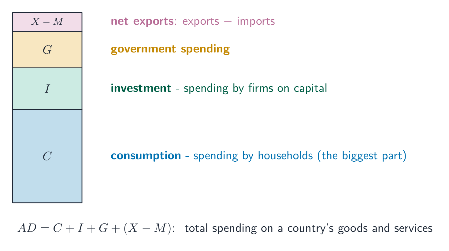
Aggregate demand (AD) 总需求 shows the total quantity of real output ($C+I+G+X_n$) buyers want at each price level 价格水平. It slopes downward for three reasons special to the whole economy:

  • the wealth effect 财富效应 (a higher price level shrinks the real value of money, so people buy less),
  • the interest-rate effect 利率效应 (a higher price level raises money demand and interest rates, cutting investment),
  • the net-export effect (a higher domestic price level makes exports dearer and imports cheaper).

A change in the price level is a movement along AD. AD shifts when any component of $C+I+G+X_n$ changes for another reason – consumer confidence, business expectations, government spending, taxes, or foreign incomes.

ไทย
แนวฟ้าเมือง: ผลผลิตรวมและità demand สะท้อนการใช้จ่ายทั้งเศรษฐกิจ
โมเดล AD–AS: การกระแทกด้านความต้องการ

ità demand (AD) แสดงปริมาณรวมของผลผลิตจริง ($C+I+G+X_n$) ที่ผู้ซื้อต้องการในแต่ละ ระดับราคา มันมีความชัน ลง ด้วยสามเหตุผลเฉพาะสำหรับเศรษฐกิจทั้งหมด:

ità demand คือการใช้จ่ายรวม: การบริโภค, การลงทุน, รัฐบาล, และการส่งออกสุทธิ
  • ผลของความมั่งคั่ง (ระดับราคาที่สูงขึ้นทำให้มูลค่าจริงของเงินลดลง ทำให้ผู้คนซื้อน้อยลง),
  • ผลของอัตราดอกเบี้ย (ระดับราคาที่สูงขึ้นเพิ่มความต้องการเงินและอัตราดอกเบี้ย ลดการลงทุน),
  • ผลของการส่งออกสุทธิ (ระดับราคาภายในประเทศที่สูงขึ้นทำให้สินค้าส่งออกแพงขึ้นและสินค้านำเข้าถูกขึ้น).

การเปลี่ยนแปลงระดับราคาคือ การเคลื่อนที่ตามเส้น AD. เส้น AD จะ เลื่อนไป เมื่อองค์ประกอบใด ๆ ของ $C+I+G+X_n$ เปลี่ยนแปลงด้วยเหตุผลอื่น – ความเชื่อมั่นของผู้บริโภค, ความคาดหวังของธุรกิจ, การใช้จ่ายของรัฐบาล, ภาษี, หรือรายได้ต่างประเทศ.

3.2

The Spending and Tax Multipliers · ⁨ตัวคูณการใช้จ่ายและตัวคูณภาษี⁩

Syllabus · ⁨หลักสูตร⁩
English

Enduring Understanding (MOD-2): Economists use the aggregate demand–aggregate supply model to represent the relationship between the price level and aggregate output in an economy and to illustrate how output, employment, and the price level respond to macroeconomic shocks.

Learning Objective MOD-2.B: a. Define the expenditure multiplier, the tax multiplier, the marginal propensity to consume, and the marginal propensity to save. b. Explain how changes in spending and taxes lead to changes in real GDP. c. Calculate how changes in spending and taxes lead to changes in real GDP.

  • MOD-2.B.1 A $\$1$ change to autonomous expenditures leads to further changes in total expenditures and total output.
  • MOD-2.B.2 The expenditure multiplier quantifies the size of the change in aggregate demand as a result of a change in any of the components of aggregate demand.
  • MOD-2.B.3 The tax multiplier quantifies the size of the change in aggregate demand as a result of a change in taxes.
  • MOD-2.B.4 The expenditure multiplier and tax multiplier depend on the marginal propensity to consume.
  • MOD-2.B.5 The marginal propensity to consume is the change in consumer spending divided by the change in disposable income. The sum of the marginal propensity to consume and marginal propensity to save is equal to one.
ไทย

ความเข้าใจที่ยั่งยืน (MOD-2): นักเศรษฐศาสตร์ใช้โมเดลความต้องการรวม–อุปทานรวม เพื่อแสดงความสัมพันธ์ระหว่างระดับราคาและผลผลิตรวมในเศรษฐกิจ และเพื่อแสดงวิธีการที่ผลผลิต การจ้างงาน และระดับราคา ตอบสนองต่อแรงกระแทกทางมหภาค

วัตถุประสงค์การเรียนรู้ MOD-2.B: ก. นิยาม ตัวคูณค่าใช้จ่าย, ตัวคูณภาษี, อัตราการบริโภคเพิ่ม边际 และอัตราการใช้เงินออมเพิ่ม边际 ข. อธิบาย (โดยใช้กราฟเมื่อเหมาะสม) ว่าการเปลี่ยนแปลงในการใช้จ่ายและภาษีนำไปสู่การเปลี่ยนแปลงใน GDP จริงได้อย่างไร ค. คำนวณ (โดยใช้กราฟเมื่อเหมาะสม) ว่าการเปลี่ยนแปลงในการใช้จ่ายและภาษีนำไปสู่การเปลี่ยนแปลงใน GDP จริงได้อย่างไร

  • MOD-2.B.1 การเปลี่ยนแปลง $\$1$ ในการใช้จ่ายอัตโนมัติ นำไปสู่การเปลี่ยนแปลงเพิ่มเติมในค่าใช้จ่ายรวมและผลผลิตรวม
  • MOD-2.B.2 ตัวคูณค่าใช้จ่าย บ่งบอกขนาดของการเปลี่ยนแปลงความต้องการรวม كنتيجةจากการเปลี่ยนแปลงในองค์ประกอบใดองค์หนึ่งของความต้องการรวม
  • MOD-2.B.3 ตัวคูณภาษี บ่งบอกขนาดของการเปลี่ยนแปลงความต้องการรวม كنتيجةจากการเปลี่ยนแปลงในภาษี
  • MOD-2.B.4 ตัวคูณค่าใช้จ่ายและตัวคูณภาษีขึ้นอยู่กับอัตราการบริโภคเพิ่ม边际
  • MOD-2.B.5 อัตราการบริโภคเพิ่ม边际 คือการเปลี่ยนแปลงในการใช้จ่ายของผู้บริโภคหารด้วยการเปลี่ยนแปลงในรายได้สุทธิ ผลรวมของอัตราการบริโภคเพิ่ม边际และอัตราการใช้เงินออมเพิ่ม边际 มีค่าเท่ากับหนึ่ง

Source: College Board AP Course and Exam Description · ⁨แหล่งที่มา: คำอธิบายหลักสูตรและข้อสอบ College Board AP⁩

English
The spending multiplier

A change in spending sets off further rounds of spending, so the final change in GDP is larger than the initial change – the multiplier effect 乘数效应. It depends on the marginal propensity to consume 边际消费倾向 (MPC), the fraction of extra income that is spent (the rest is the marginal propensity to save 边际储蓄倾向, MPS, with $MPC+MPS=1$):

$$\text{spending multiplier}=\frac{1}{1-MPC}=\frac{1}{MPS}.$$

A tax cut works through the multiplier too, but more weakly, because part of the tax cut is saved:

$$\text{tax multiplier}=-\frac{MPC}{1-MPC}=-\frac{MPC}{MPS}.$$

The tax multiplier is smaller in size and negative (a tax cut raises GDP; a tax rise lowers it). Total change in GDP $=$ (multiplier) $\times$ (initial change).

Worked example. If $MPC=0.8$, the spending multiplier is $\dfrac{1}{1-0.8}=5$, so a $\$10$ billion rise in government spending lifts real GDP by $5\times\$10=\$50$ billion. The tax multiplier is $-\dfrac{0.8}{0.2}=-4$, so a $\$10$ billion tax cut raises GDP by only $\$40$ billion – weaker, because part of the tax cut is saved.

Exam skill: compute both multipliers from the MPC and find the resulting change in real GDP – an almost-guaranteed calculation.

ไทย
ตัวคูณการใช้จ่าย

การเปลี่ยนแปลงในการใช้จ่ายจะกระตุ้นให้เกิดรอบของการใช้จ่ายเพิ่มเติม ดังนั้นการเปลี่ยนแปลงสุดท้ายใน GDP จึงมีขนาด มากกว่า การเปลี่ยนแปลงเริ่มต้น – นี่คือ ผลคูณ. มันขึ้นอยู่กับ ** propensity to consume边际 (MPC)**, คือสัดส่วนของรายได้เพิ่มเติมที่ถูกใช้จ่าย (ส่วนที่เหลือคือ propensity to save边际, MPS, โดยมี $MPC+MPS=1$):

การแทรกซึมหนึ่งครั้งขยายเป็นผลรวมการเพิ่มขึ้นของรายได้อย่างมีนัยสำคัญ
$$\text{spending multiplier}=\frac{1}{1-MPC}=\frac{1}{MPS}.$$

การลดภาษีทำงานผ่านตัวคูณเช่นกัน แต่มีผลอ่อนกว่า เนื่องจากบางส่วนของภาษีที่ลดได้จะถูกเก็บออมไว้:

$$\text{tax multiplier}=-\frac{MPC}{1-MPC}=-\frac{MPC}{MPS}.$$

ตัวคูณภาษีมีขนาด เล็กกว่า และเป็น ลบ (การลดภาษีเพิ่ม GDP; การเพิ่มภาษีลด GDP) การเปลี่ยนแปลงรวมใน GDP $=$ (ตัวคูณ) $\times$ (การเปลี่ยนแปลงเริ่มต้น).

ตัวอย่างฝึกฝน. ถ้า $MPC=0.8$, ตัวคูณการใช้จ่ายคือ $\dfrac{1}{1-0.8}=5$, ดังนั้นการลดภาษี $\$10$ billion rise in government spending lifts real GDP by $5\times\$10=\$50$ billion. The tax multiplier is $-\dfrac{0.8}{0.2}=-4$, so a $\$10$ พันล้านดอลลาร์สหรัฐ จะเพิ่ม GDP เพียง $\$40$ พันล้านดอลลาร์สหรัฐ – มีผลอ่อนกว่า เพราะบางส่วนของการลดภาษีถูกเก็บออมไว้.

เทคนิคการสอบ: คำนวณตัวคูณทั้งสองจาก MPC และหาการเปลี่ยนแปลงของ GDP จริง – เป็นการคำนวณที่แทบจะแน่นอนที่จะออกสอบ.

Explore · ⁨สำรวจ⁩

See the spending multiplier ripple out · ⁨เห็นผลกระทบคูณของการใช้จ่ายที่แผ่ขยายออกไป⁩

A dollar of new spending becomes someone's income, part of which they spend again — so the total effect is a multiple of the first injection, set by the marginal propensity to consume (MPC). · ⁨เงินหนึ่งดอลลาร์จากการใช้จ่ายใหม่กลายเป็นรายได้ของคนอื่น คนหนึ่งบางส่วนถูกนำไปใช้จ่ายอีกครั้ง — ดังนั้นผลกระทบรวมจึงเป็น หลายเท่า ของการฉีดเข้าครั้งแรก ซึ่งกำหนดโดยอัตราการบริโภครายได้เพิ่ม (MPC)⁩

3.3

Short-Run Aggregate Supply · ⁨Oferta รวมระยะสั้น⁩

Syllabus · ⁨หลักสูตร⁩
English

Enduring Understanding (MOD-2): Economists use the aggregate demand–aggregate supply model to represent the relationship between the price level and aggregate output in an economy and to illustrate how output, employment, and the price level respond to macroeconomic shocks.

Learning Objective MOD-2.C: a. Define (using graphs as appropriate) the short-run aggregate supply (SRAS) curve. b. Explain (using graphs as appropriate) the slope of the SRAS curve and its determinants.

  • MOD-2.C.1 The short-run aggregate supply (SRAS) curve describes the relationship between the price level and the quantity of goods and services supplied in an economy.
  • MOD-2.C.2 The SRAS curve is upward-sloping because of sticky wages and prices. [See EK MOD-2.E.1]
  • MOD-2.C.3 Any factor that causes production costs to change, such as a change in inflationary expectations, will cause the SRAS curve to shift.

Learning Objective MOD-2.D: Explain (using graphs as appropriate) how movement along the SRAS curve implies a relationship between the price level (and inflation) and unemployment.

  • MOD-2.D.1 Moving along the SRAS curve, an increase in the price level is associated with an increase in output, which means employment must correspondingly rise. With the labor force held constant, unemployment will fall. So, there is a short-run trade-off between inflation and unemployment. [See EK MOD-3.A.1]
ไทย

ความเข้าใจที่ยั่งยืน (MOD-2): นักเศรษฐศาสตร์ใช้โมเดลความต้องการรวม–อุปทานรวม เพื่อแสดงความสัมพันธ์ระหว่างระดับราคาและผลผลิตรวมในเศรษฐกิจ และเพื่อแสดงวิธีการที่ผลผลิต การจ้างงาน และระดับราคา ตอบสนองต่อแรงกระแทกทางมหภาค

วัตถุประสงค์การเรียนรู้ MOD-2.C: ก. นิยาม (โดยใช้กราฟเมื่อเหมาะสม) เส้นอุปทานรวมระยะสั้น (SRAS) ข. อธิบาย (โดยใช้กราฟเมื่อเหมาะสม) ความชันของเส้น SRAS และปัจจัยกำหนด

  • MOD-2.C.1 เส้นอุปทานรวมระยะสั้น (SRAS) แสดงความสัมพันธ์ระหว่างระดับราคาและปริมาณสินค้าและบริการที่เสนอขายในเศรษฐกิจ
  • MOD-2.C.2 เส้น SRAS มีความชันเป็นบวกเนื่องจากค่าจ้างและราคาที่ติดขัด [ดู EK MOD-2.E.1]
  • MOD-2.C.3 ปัจจัยใดๆ ที่ทำให้ต้นทุนการผลิตเปลี่ยนแปลง เช่น การเปลี่ยนแปลงความคาดหวังเรื่องเงินเฟ้อ จะทำให้เส้น SRAS เลื่อนไป

วัตถุประสงค์การเรียนรู้ MOD-2.D: อธิบาย (โดยใช้กราฟเมื่อเหมาะสม) ว่าการเคลื่อนที่ตามเส้น SRAS implicates ความสัมพันธ์ระหว่างระดับราคา (และเงินเฟ้อ) กับอัตราการว่างงานอย่างไร

  • MOD-2.D.1 เมื่อเคลื่อนที่ตามเส้น SRAS การเพิ่มขึ้นของระดับราคาสัมพันธ์กับการเพิ่มขึ้นของผลผลิต ซึ่งหมายความว่าต้องมีการจ้างงานเพิ่มขึ้นด้วย หากแรงงานคงที่ อัตราการว่างงานจะลดลง ดังนั้นจึงมีความแลกกันระยะสั้นระหว่างเงินเฟ้อและการว่างงาน [ดู EK MOD-3.A.1]

Source: College Board AP Course and Exam Description · ⁨แหล่งที่มา: คำอธิบายหลักสูตรและข้อสอบ College Board AP⁩

English

Short-run aggregate supply (SRAS) 短期总供给 slopes upward: in the short run some input prices (especially nominal wages 名义工资) are sticky 粘性, so a higher output price level widens profit margins and firms produce more. SRAS shifts with input prices, productivity, taxes/subsidies on producers, and supply shocks (e.g. an oil-price change). A rise in input costs shifts SRAS left.

ไทย
โรงงานไฟฟ้าและพื้นที่อุตสาหกรรม: อุปทานรวมระยะสั้นขึ้นอยู่กับต้นทุนการผลิต

อุปทานรวมระยะสั้น (SRAS) มีแนวโน้ม ยกตัวขึ้น: ในระยะสั้น ราคาปัจจัยการผลิตบางอย่าง (โดยเฉพาะ ค่าจ้าง nomi nal) มีความ เหนียวเหนอะหนะ, ดังนั้นเมื่อระดับราคาสินค้าสูงขึ้นจะทำให้ส่วนต่างกำไรกว้างขึ้น และบริษัทจะผลิตมากขึ้น SRAS จะ เลื่อนไป ตาม ราคาปัจจัยการผลิต, ประสิทธิภาพการผลิต, ภาษี/เงินอุดหนุนสำหรับผู้ผลิต, และ แรงกระแทกด้านอุปทาน (เช่น การเปลี่ยนแปลงราคาน้ำมัน) การเพิ่มขึ้นของต้นทุนการผลิตจะเลื่อน SRAS ไปทางซ้าย.

3.4

Long-Run Aggregate Supply · ⁨Oferta รวมระยะยาว⁩

Syllabus · ⁨หลักสูตร⁩
English

Enduring Understanding (MOD-2): Economists use the aggregate demand–aggregate supply model to represent the relationship between the price level and aggregate output in an economy and to illustrate how output, employment, and the price level respond to macroeconomic shocks.

Learning Objective MOD-2.E: Define (using graphs as appropriate) the short run and the long run.

  • MOD-2.E.1 In the long run all prices and wages are fully flexible, while in the short run some input prices are fixed. A consequence of flexible long-run prices and wages is the lack of a long-run trade-off between inflation and unemployment.

Learning Objective MOD-2.F: Define (using graphs as appropriate) the long-run aggregate supply (LRAS) curve.

  • MOD-2.F.1 The LRAS curve corresponds to the production possibilities curve (PPC) because they both represent maximum sustainable capacity. Maximum sustainable capacity is the total output an economic system will produce over a set period of time if all resources are fully employed. [See LO MOD-2.I]
  • MOD-2.F.2 The LRAS curve is vertical at the full-employment level of output because in the long run wages and prices fully adjust.
ไทย

ความเข้าใจที่ยั่งยืน (MOD-2): นักเศรษฐศาสตร์ใช้โมเดลความต้องการรวม–อุปทานรวม เพื่อแสดงความสัมพันธ์ระหว่างระดับราคาและผลผลิตรวมในเศรษฐกิจ และเพื่อแสดงวิธีการที่ผลผลิต การจ้างงาน และระดับราคา ตอบสนองต่อแรงกระแทกทางมหภาค

วัตถุประสงค์การเรียนรู้ MOD-2.E: นิยาม (โดยใช้กราฟเมื่อเหมาะสม) ระยะสั้นและระยะยาว

  • MOD-2.E.1 ในระยะยาว ราคาและค่าจ้างทั้งหมดปรับได้เต็มที่ ในขณะที่ในระยะสั้น ราคาปัจจัยการผลิตบางชนิดถูกผูกไว้ ผลลัพธ์จากราคาและค่าจ้างที่ปรับได้ในระยะยาวคือไม่มีความแลกกันระหว่างเงินเฟ้อและการว่างงานในระยะยาว

วัตถุประสงค์การเรียนรู้ MOD-2.F: นิยาม (โดยใช้กราฟเมื่อเหมาะสม) เส้นอุปทานรวมระยะยาว (LRAS)

  • MOD-2.F.1 เส้น LRAS สอดคล้องกับเส้นความเป็นไปได้ในการผลิต (PPC) เพราะทั้งสองแสดงถึงกำลังการผลิตที่ยั่งยืนสูงสุด กำลังการผลิตที่ยั่งยืนสูงสุดคือผลผลิตรวมที่ระบบเศรษฐกิจจะผลิตในช่วงเวลาที่กำหนดหากมีการใช้ทรัพยากรอย่างเต็มที่ [ดู LO MOD-2.I]
  • MOD-2.F.2 เส้น LRAS เป็นแนวตั้งที่ระดับผลผลิตของการจ้างงานเต็ม เนื่องจากในระยะยาวค่าจ้างและราคาปรับได้อย่างเต็มที่

Source: College Board AP Course and Exam Description · ⁨แหล่งที่มา: คำอธิบายหลักสูตรและข้อสอบ College Board AP⁩

English

Long-run aggregate supply (LRAS) 长期总供给 is vertical at the economy's full-employment (potential) output 潜在产出 $Y_f$. In the long run all prices and wages are fully flexible (only in the short run are some input prices fixed), so output depends only on real factors – resources, technology, institutions – not the price level. LRAS shifts only with economic growth (more or better resources). LRAS corresponds to the production possibilities curve (PPC) 生产可能性曲线: both mark the economy's maximum sustainable capacity, so an outward LRAS shift and an outward PPC shift are the same event drawn two ways. The vertical LRAS is why, in the long run, demand policy changes prices, not output.

ไทย

อุปทานรวมระยะยาว (LRAS) เป็นเส้น ตั้งตรง ที่ระดับ ผลผลิตเต็มกำลัง (ผลผลิตศักยภาพ) $Y_f$ ของเศรษฐกิจ ในระยะยาว ทุก ราคาและค่าจ้างมีความ ยืดหยุ่น อย่างเต็มที่ (มีการกำหนดราคาปัจจัยผลิตคงที่เฉพาะในระยะสั้นเท่านั้น) ดังนั้นผลผลิตจึงขึ้นอยู่กับปัจจัยจริง – ทรัพยากร, เทคโนโลยี, สถาบัน – ไม่ใช่ระดับราคา LRAS เลื่อนไปเพียงเมื่อเกิด การเติบโตทางเศรษฐกิจ (ทรัพยากรมากขึ้นหรือดีขึ้น) LRAS สอดคล้องกับ เส้นความสามารถในการผลิต (PPC): ทั้งสองชี้ถึง ขีดความสามารถที่ยั่งยืนสูงสุด ของเศรษฐกิจ ดังนั้นการเลื่อน LRAS ออกไปและการเลื่อน PPC ออกไปจึงเป็นเหตุการณ์เดียวกันที่วาดออกมาสองรูปแบบ เส้นตั้งตรงของ LRAS คือสาเหตุที่ว่าในระยะยาว นโยบายด้านอุปสงค์จะเปลี่ยนราคา ไม่ใช่ผลผลิต.

นโยบายด้านอุปทานเลื่อนอุปทานรวมระยะยาวไปทางขวา: ผลผลิตมากขึ้น ราคาต่ำลง
3.5

Equilibrium in the AD-AS Model · ⁨จุดสมดุลในโมเดล AD-AS⁩

Syllabus · ⁨หลักสูตร⁩
English

Enduring Understanding (MOD-2): Economists use the aggregate demand–aggregate supply model to represent the relationship between the price level and aggregate output in an economy and to illustrate how output, employment, and the price level respond to macroeconomic shocks.

Learning Objective MOD-2.G: Explain (using graphs as appropriate) the short-run and long-run equilibrium price level and output level.

  • MOD-2.G.1 Short-run equilibrium occurs when the aggregate quantity of output demanded and the aggregate quantity of output supplied are equal—i.e., at the intersection of the AD and SRAS curves.
  • MOD-2.G.2 Long-run equilibrium occurs when the AD and SRAS curves intersect on the LRAS—i.e., at the full-employment level of real output.
  • MOD-2.G.3 The short-run equilibrium output can be at the full-employment level of output, above it, or below it, creating positive (i.e., inflationary) or negative (i.e., recessionary) output gaps.
ไทย

ความเข้าใจที่ยั่งยืน (MOD-2): นักเศรษฐศาสตร์ใช้โมเดลความต้องการรวม–อุปทานรวม เพื่อแสดงความสัมพันธ์ระหว่างระดับราคาและผลผลิตรวมในเศรษฐกิจ และเพื่อแสดงวิธีการที่ผลผลิต การจ้างงาน และระดับราคา ตอบสนองต่อแรงกระแทกทางมหภาค

วัตถุประสงค์การเรียนรู้ MOD-2.G: อธิบาย (โดยใช้กราฟเมื่อเหมาะสม) ระดับราคาและระดับผลผลิตในจุดสมดุลระยะสั้นและระยะยาว

  • MOD-2.G.1 จุดสมดุลระยะสั้นเกิดขึ้นเมื่อปริมาณผลผลิตที่ต้องการรวมและปริมาณผลผลิตที่เสนอรวมเท่ากัน—นั่นคือ ที่จุดตัดของเส้น AD และ SRAS
  • MOD-2.G.2 จุดสมดุลระยะยาวเกิดขึ้นเมื่อเส้น AD และ SRAS ตัดกันบนเส้น LRAS—นั่นคือ ที่ระดับผลผลิตจริงของการจ้างงานเต็ม
  • MOD-2.G.3 ผลผลิตในจุดสมดุลระยะสั้นอาจอยู่ที่ระดับผลผลิตของการจ้างงานเต็ม เหนือระดับนั้น หรือต่ำกว่าระดับนั้น ทำให้เกิดช่องว่างผลผลิตเชิงบวก (เช่น ช่องว่างเงินเฟ้อ) หรือช่องว่างผลผลิตเชิงลบ (เช่น ช่องว่างSETTING recessionary)

Source: College Board AP Course and Exam Description · ⁨แหล่งที่มา: คำอธิบายหลักสูตรและข้อสอบ College Board AP⁩

English

The economy settles where AD meets SRAS, fixing the equilibrium price level and real GDP. Comparing that output to $Y_f$ (the LRAS line) gives the economy's state:

  • output $: a recessionary gap 衰退缺口 (cyclical unemployment),
  • output $>Y_f$: an inflationary gap 通胀缺口 (overheating),
  • output $=Y_f$: long-run equilibrium.
ไทย

เศรษฐกิจจะเข้าสู่สภาวะสมดุลเมื่อ AD ตัดกับ SRAS, ซึ่งกำหนด ระดับราคาสมดุล และ GDP จริง การเปรียบเทียบผลผลิตนั้นกับ $Y_f$ (เส้น LRAS) บอกสถานะของเศรษฐกิจ:

ความสมดุลทางมหภาคเมื่ออุปสงค์รวมตัดกับอุปทานรวม
  • ผลผลิต $: เกิด ช่องว่างช่วง recessionary (การว่างงานแบบวัฏจักร),
  • ผลผลิต $>Y_f$: เกิด ช่องว่างช่วง inflationary (เศรษฐกิจร้อนแรงเกิน),
  • ผลผลิต $=Y_f$: สภาวะสมดุลระยะยาว.
Explore · ⁨สำรวจ⁩

Find equilibrium in the AD-AS model · ⁨หาจุดสมดุลในโมเดล AD-AS⁩

Aggregate demand and aggregate supply cross at the economy's price level and real GDP. A demand or supply shock shifts a curve and moves the whole economy's output and prices. · ⁨** Aggregate demand** และ aggregate supply ตัดกันที่ระดับราคาและ GDP จริงของเศรษฐกิจ การกระแทกจากฝั่งความต้องการหรือ供给侧จะเลื่อนเส้นและเปลี่ยนผลผลิตและราคาของเศรษฐกิจทั้งระบบ⁩

3.6

Short-Run Changes: Demand and Supply Shocks · ⁨การเปลี่ยนแปลงระยะสั้น: แรงกระตุ้นด้านความต้องการและofferta⁩

Syllabus · ⁨หลักสูตร⁩
English

Enduring Understanding (MOD-2): Economists use the aggregate demand–aggregate supply model to represent the relationship between the price level and aggregate output in an economy and to illustrate how output, employment, and the price level respond to macroeconomic shocks.

Learning Objective MOD-2.H: Explain (using graphs as appropriate) the response of output, employment, and the price level to an aggregate demand or aggregate supply shock in the short run.

  • MOD-2.H.1 A positive (negative) shock in AD causes output, employment, and the price level to rise (fall) in the short run.
  • MOD-2.H.2 A positive (negative) shock in SRAS causes output and employment to rise (fall) and the price level to fall (rise) in the short run.
  • MOD-2.H.3 Inflation can be caused by changes in aggregate demand (demand-pull) or aggregate supply (cost-push).
ไทย

ความเข้าใจที่ยั่งยืน (MOD-2): นักเศรษฐศาสตร์ใช้โมเดลความต้องการรวม–อุปทานรวม เพื่อแสดงความสัมพันธ์ระหว่างระดับราคาและผลผลิตรวมในเศรษฐกิจ และเพื่อแสดงวิธีการที่ผลผลิต การจ้างงาน และระดับราคา ตอบสนองต่อแรงกระแทกทางมหภาค

วัตถุประสงค์การเรียนรู้ MOD-2.H: อธิบาย (โดยใช้กราฟเมื่อเหมาะสม) การตอบสนองของผลผลิต การจ้างงาน และระดับราคาต่อแรงกระแทกด้านความต้องการรวมหรืออุปทานรวมในระยะสั้น

  • MOD-2.H.1 การกระแทกใน AD เป็นบวก (ลบ) ทำให้ผลผลิต การจ้างงาน และระดับราคาเพิ่มขึ้น (ลดลง) ในระยะสั้น
  • MOD-2.H.2 การกระแทกใน SRAS เป็นบวก (ลบ) ทำให้ผลผลิตและการจ้างงานเพิ่มขึ้น (ลดลง) และระดับราคาลดลง (เพิ่มขึ้น) ในระยะสั้น
  • MOD-2.H.3 เงินเฟ้ออาจเกิดจากการเปลี่ยนแปลงของอุปสงค์รวม (demand-pull) หรืออุปทานรวม (cost-push)

Source: College Board AP Course and Exam Description · ⁨แหล่งที่มา: คำอธิบายหลักสูตรและข้อสอบ College Board AP⁩

English
  • A demand shock shifts AD: a positive one (more spending) raises both price level and output (and lowers unemployment); a negative one lowers both.
  • A supply shock shifts SRAS: a negative one (higher input costs) raises the price level and lowers output at once – stagflation 滞胀 – the hardest case for policymakers, because fixing one worsens the other.
ไทย
  • แรงกระแทกด้านอุปสงค์ เลื่อน AD: แบบบวก (การใช้จ่ายเพิ่มขึ้น) เพิ่มทั้งระดับราคาและผลผลิต (และลดการว่างงาน); แบบลบลดทั้งสองอย่าง.
  • แรงกระแทกด้านอุปทาน เลื่อน SRAS: แบบลบ (ต้นทุนปัจจัยผลิตสูงขึ้น) เพิ่มระดับราคา และ ลดผลผลิตพร้อมกัน – stagflation – ซึ่งเป็นสถานการณ์ที่ยากที่สุดสำหรับผู้กำหนดนโยบาย เพราะการแก้ไขอย่างหนึ่งจะยิ่งทำให้อีกอย่างแย่ลง.
Vocabulary · ⁨คำศัพท์⁩ Train · ⁨ฝึกฝน⁩
English ไทย
stagflation/stæɡˈfleɪʃn/ stagflation
3.7

Long-Run Self-Adjustment · ⁨การปรับตัวเองในระยะยาว⁩

Syllabus · ⁨หลักสูตร⁩
English

Enduring Understanding (MOD-2): Economists use the aggregate demand–aggregate supply model to represent the relationship between the price level and aggregate output in an economy and to illustrate how output, employment, and the price level respond to macroeconomic shocks.

Learning Objective MOD-2.I: Explain (using graphs as appropriate) the response of output, employment, and the price level to an aggregate demand or aggregate supply shock in the long run.

  • MOD-2.I.1 In the long run, in the absence of government policy actions, flexible wages and prices will adjust to restore full employment and unemployment will revert to its natural rate after a shock to aggregate demand or short-run aggregate supply. [See EK MEA-1.E.2]
  • MOD-2.I.2 Shifts in the long-run aggregate supply curve indicate changes in the full-employment level of output and economic growth.
ไทย

ความเข้าใจที่ยั่งยืน (MOD-2): นักเศรษฐศาสตร์ใช้โมเดลความต้องการรวม–อุปทานรวม เพื่อแสดงความสัมพันธ์ระหว่างระดับราคาและผลผลิตรวมในเศรษฐกิจ และเพื่อแสดงวิธีการที่ผลผลิต การจ้างงาน และระดับราคา ตอบสนองต่อแรงกระแทกทางมหภาค

จุดประสงค์การเรียนรู้ MOD-2.I: อธิบาย (โดยใช้กราฟเมื่อจำเป็น) ผลกระทบต่อผลผลิต การจ้างงาน และระดับราคาต่อการกระแทกของอุปสงค์รวมหรืออุปทานรวมในระยะยาว

  • MOD-2.I.1 ในระยะยาว หากไม่มีการดำเนินการนโยบายจากรัฐบาล ค่าจ้างและราคาที่ยืดหยุ่นจะปรับตัวเพื่อคืนการจ้างงานเต็มรูปแบบ และการว่างงานจะกลับสู่อัตราธรรมชาติหลังจากเกิดการกระแทกต่ออุปสงค์รวมหรืออุปทานรวมระยะสั้น [ดู EK MEA-1.E.2]
  • MOD-2.I.2 การเคลื่อนตัวของเส้นอุปทานรวมระยะยาวบ่งชี้ถึงการเปลี่ยนแปลงของระดับผลผลิตที่จ้างงานเต็มรูปแบบและการเติบโตทางเศรษฐกิจ

Source: College Board AP Course and Exam Description · ⁨แหล่งที่มา: คำอธิบายหลักสูตรและข้อสอบ College Board AP⁩

English

Left alone, the economy self-corrects through flexible wages:

  • In a recessionary gap, high unemployment eventually pushes nominal wages down, shifting SRAS right until output returns to $Y_f$ at a lower price level.
  • In an inflationary gap, labor shortages push wages up, shifting SRAS left back to $Y_f$ at a higher price level.

The debate over how fast this happens is the case for (or against) active policy: self-adjustment is slow and painful, which is the argument for intervening.

ไทย

หากปล่อยไว้ตามธรรมชาติ เศรษฐกิจจะปรับตัวเองผ่านค่าจ้างที่ยืดหยุ่น:

  • ใน ช่องว่างช่วง recessionary การว่างงานสูงในที่สุดก็จะกดดันให้ ค่าจ้าง nomi nal ลดลง, เลื่อน SRAS ไปทางขวา จนผลผลิตกลับสู่ $Y_f$ ที่ระดับราคาต่ำกว่า.
  • ใน ช่องว่างช่วง inflationary การขาดแคลนแรงงานจะดันให้ ค่าจ้างสูงขึ้น, เลื่อน SRAS ไปทางซ้าย กลับสู่ $Y_f$ ที่ระดับราคาสูงกว่า.

ข้อถกเถียงเกี่ยวกับ ความเร็ว ของกระบวนการนี้คือประเด็นสำหรับการใช้ илиไม่ใช้นโยบายเชิงรุก: การปรับตัวเองนั้นช้าและเจ็บปวด ซึ่งเป็นเหตุผลสนับสนุนการแทรกแซง.

3.8

Fiscal Policy · ⁨นโยบายการคลัง⁩

Syllabus · ⁨หลักสูตร⁩
English

Enduring Understanding (POL-1): Fiscal and monetary policy have short-run effects on macroeconomic outcomes.

Learning Objective POL-1.A: a. Define fiscal policy and related terms. b. Explain (using graphs as appropriate) the short-run effects of a fiscal policy action. c. Calculate the short-run effects of a fiscal policy action.

  • POL-1.A.1 Governments implement fiscal policies to achieve macroeconomic goals, such as full employment.
  • POL-1.A.2 The tools of fiscal policy are government spending and taxes/transfers.
  • POL-1.A.3 Changes in government spending affect aggregate demand directly, and changes in taxes/transfers affect aggregate demand indirectly.
  • POL-1.A.4 The government spending multiplier is greater than the tax multiplier.
  • POL-1.A.5 Expansionary or contractionary fiscal policies are used to restore full employment when the economy is in a negative (i.e., recessionary) or positive (i.e., inflationary) output gap.
  • POL-1.A.6 Fiscal policy can influence aggregate demand, real output, and the price level. [See also EK MKT-5.E.2 for the effect on exchange rates.]
  • POL-1.A.7 The AD–AS model is used to demonstrate the short-run effects of fiscal policy.

Learning Objective POL-1.B: Define why there are lags to discretionary fiscal policy.

  • POL-1.B.1 In reality, there are lags to discretionary fiscal policy because of factors such as the time it takes to decide on and implement a policy action.
ไทย

ความเข้าใจที่ยั่งยืน (POL-1): นโยบายการเงินและนโยบายการคลังมีผลกระทบระยะสั้นต่อผลลัพธ์ทางมหภาค

จุดประสงค์การเรียนรู้ POL-1.A: a. นิยามนโยบายการคลังและคำศัพท์ที่เกี่ยวข้อง b. อธิบาย (โดยใช้กราฟเมื่อจำเป็น) ผลกระทบระยะสั้นของการดำเนินการนโยบายการคลัง c. คำนวณผลกระทบระยะสั้นของการดำเนินการนโยบายการคลัง

  • POL-1.A.1 รัฐบาลดำเนินนโยบายการคลังเพื่อให้บรรลุเป้าหมายทางมหภาค เช่น การจ้างงานเต็มรูปแบบ
  • POL-1.A.2 เครื่องมือของนโยบายการคลังคือรายจ่ายภาครัฐและภาษี/เงินโอน
  • POL-1.A.3 การเปลี่ยนแปลงรายจ่ายภาครัฐส่งผลต่ออุปสงค์รวมโดยตรง และการเปลี่ยนแปลงภาษี/เงินโอนส่งผลต่ออุปสงค์รวมโดยอ้อม
  • POL-1.A.4 ตัวคูณรายจ่ายภาครัฐมีค่ามากกว่าตัวคูณภาษี
  • POL-1.A.5 นโยบายการคลังแบบขยายหรือ紧缩ถูกใช้เพื่อคืนการจ้างงานเต็มรูปแบบเมื่อเศรษฐกิจอยู่ในช่องว่างผลลบ (เช่น ช่วง recessionary) หรือช่องว่างผลบวก (เช่น ช่วง inflationary)
  • POL-1.A.6 นโยบายการคลังสามารถส่งผลกระทบต่ออุปสงค์รวม ผลผลิตรวมจริง และระดับราคา [ดู EK MKT-5.E.2 สำหรับผลกระทบต่อดอกเบี้ยแลกเปลี่ยนด้วย]
  • POL-1.A.7 โมเดล AD–AS ถูกใช้เพื่อแสดงผลกระทบระยะสั้นของนโยบายการคลัง

จุดประสงค์การเรียนรู้ POL-1.B: นิยามเหตุผลที่มี thờiหน่วงในการดำเนินนโยบายการคลังแบบเลือกปฏิบัติ

  • POL-1.B.1 ในความเป็นจริง มีเวลาหน่วงในการดำเนินนโยบายการคลังแบบเลือกปฏิบัติเนื่องจากปัจจัยต่าง ๆ เช่น ระยะเวลาที่ใช้ในการตัดสินใจและดำเนินการนโยบาย

Source: College Board AP Course and Exam Description · ⁨แหล่งที่มา: คำอธิบายหลักสูตรและข้อสอบ College Board AP⁩

English

Fiscal policy 财政政策 is the government's use of spending and taxes to shift AD:

  • Expansionary 扩张性 (more spending or lower taxes) shifts AD right to close a recessionary gap.
  • Contractionary 紧缩性 (less spending or higher taxes) shifts AD left to close an inflationary gap.

Size the policy with the multipliers: to close a gap of a given size, the required change in spending is (gap) $\div$ (spending multiplier). Limits include time lags, crowding out (below), and political difficulty.

Worked example. An economy has a $\$100$ billion recessionary gap and $MPC=0.75$ (spending multiplier $=\dfrac{1}{0.25}=4$). To close it, the government must raise spending by $\dfrac{\$100\text{ billion}}{4}=\$25$ billion. Using a tax cut instead (tax multiplier $-3$) would require a larger $\dfrac{100}{3}\approx\$33$ billion cut.

Exam skill: you must draw the correctly labeled AD-AS graph, identify the gap, prescribe the right fiscal action and its direction, and often calculate the exact spending or tax change needed.

ไทย

นโยบายการคลัง คือการใช้ การใช้จ่าย และ ภาษี ของรัฐบาลเพื่อเลื่อน AD:

นโยบายการคลังแบบขยายเลือน AD ไปทางขวา เพิ่มผลผลิตและราคา
  • แบบขยาย (เพิ่มการใช้จ่ายหรือลดภาษี) เลือน AD ไปทางขวา เพื่อปิด ช่องว่าง recessionary.
  • แบบหดตัว (ลดการใช้จ่ายหรือเพิ่มภาษี) เลือน AD ไปทางซ้าย เพื่อปิด ช่องว่าง inflationary.

ปรับขนาดนโยบายด้วยตัวคูณ: ในการปิดช่องว่างที่มีขนาดที่กำหนด การเปลี่ยนแปลงในการใช้จ่ายที่ต้องการคือ (ช่องว่าง) $\div$ (ตัวคูณการใช้จ่าย) ข้อจำกัดรวมถึง ช่วงเวลาล่าช้า, crowding out (ด้านล่าง), และความยากทางการเมือง.

ตัวอย่างที่คำนวณแล้ว. เศรษฐกิจมี $\$100$ billion recessionary gap and $MPC=0.75$ (spending multiplier $=\dfrac{1}{0.25}=4$). To close it, the government must raise spending by $\dfrac{\$100\text{ billion}}{4}=\$25$ billion. Using a tax cut instead (tax multiplier $-3$) would require a larger $\dfrac{100}{3}\approx\$33$ พันล้านลดลง

ทักษะการสอบ: คุณต้องวาดกราฟ AD-AS ที่มีการระบุชื่อถูกต้อง ระบุช่องว่าง แนะนำมาตรการ fiscal ที่เหมาะสมและทิศทางของมัน และมักจะต้องคำนวณการเปลี่ยนแปลงของรายจ่ายหรือภาษีที่จำเป็นให้แม่นยำ

Vocabulary · ⁨คำศัพท์⁩ Train · ⁨ฝึกฝน⁩
English ไทย
recessionary gap/rɪˈseʃənəri ɡæp/ ช่องว่างระยะถอยกลับ
inflationary gap/ɪnˈfleɪʃənəri ɡæp/ ช่องว่างเงินเฟ้อ
Fiscal policy/ˈfɪskl ˈpɒlɪsi/ นโยบายการคลัง
Expansionary/ekˈspænʃənəri/ การขยายตัว
Contractionary/kənˈtrækʃənəri/ การหดตัว
Automatic stabilizers/ˌɔːtəˈmætɪk ˈsteɪbəlaɪzəz/ เครื่องปรับเสถียรอัตโนมัติ
3.9

Automatic Stabilizers · ⁨ระบบปรับสมดุลอัตโนมัติ (Automatic Stabilizers)⁩

Syllabus · ⁨หลักสูตร⁩
English

Enduring Understanding (POL-1): Fiscal and monetary policy have short-run effects on macroeconomic outcomes.

Learning Objective POL-1.C: a. Define automatic stabilizers. b. Explain how automatic stabilizers moderate business cycles.

  • POL-1.C.1 Automatic stabilizers support the economy during recessions and help prevent the economy from being overheated during expansionary periods.
  • POL-1.C.2 Tax revenues decrease automatically as GDP falls, preventing consumption and the economy from falling further.
  • POL-1.C.3 Tax revenues increase automatically as GDP rises, slowing consumption and preventing the economy from overheating.
  • POL-1.C.4 Government policies, institutions, or agencies may also have social service programs whose transfer payments act as automatic stabilizers.
ไทย

ความเข้าใจที่ยั่งยืน (POL-1): นโยบายการเงินและนโยบายการคลังมีผลกระทบระยะสั้นต่อผลลัพธ์ทางมหภาค

จุดประสงค์การเรียนรู้ POL-1.C: a. นิยามเครื่องมือปรับสมดุลอัตโนมัติ b. อธิบายว่าเครื่องมือปรับสมดุลอัตโนมัติช่วยลดความรุนแรงของรอบธุรกิจอย่างไร

  • POL-1.C.1 เครื่องมือปรับสมดุลอัตโนมัติช่วยสนับสนุนเศรษฐกิจในช่วง recession และช่วยป้องกันไม่ให้เศรษฐกิจร้อนเกินไปในช่วง expansionary periods
  • POL-1.C.2 รายได้ภาษีลดลงโดยอัตโนมัติเมื่อ GDP ลดลง ป้องกันไม่ให้การบริโภคและเศรษฐกิจตกลงไป更深
  • POL-1.C.3 รายได้ภาษีเพิ่มขึ้นโดยอัตโนมัติเมื่อ GDP เพิ่มขึ้น ชะลอการบริโภคและป้องกันไม่ให้เศรษฐกิจร้อนเกินไป
  • POL-1.C.4 นโยบาย institutions หรือหน่วยงานของรัฐอาจมีโปรแกรมบริการสังคมwhose transfer payments ทำหน้าที่เป็นเครื่องมือปรับสมดุลอัตโนมัติ

Source: College Board AP Course and Exam Description · ⁨แหล่งที่มา: คำอธิบายหลักสูตรและข้อสอบ College Board AP⁩

English

Automatic stabilizers 自动稳定器 are features that dampen the cycle without new legislation. In a downturn, progressive taxes collect less and transfer payments (unemployment benefits, welfare) rise automatically – cushioning incomes and spending; in a boom they do the reverse. They soften the cycle and act instantly, avoiding the lags of discretionary 相机抉择 policy.

ไทย

ระบบปรับสมดุลอัตโนมัติ คือคุณสมบัติที่ช่วยลดความผันผวนของวงจร โดยไม่มีการออกกฎหมายใหม่ ในช่วงเศรษฐกิจถดถอย ภาษีแบบขั้นบันได จะเก็บเงินได้น้อยลง และ การชำระเงินโอน (เงินประกันการว่างงาน, สวัสดิการ) จะเพิ่มขึ้นโดยอัตโนมัติ – ช่วยรองรับรายได้และการใช้จ่าย; ในช่วงเศรษฐกิจบูมจะเกิดผลตรงกันข้าม ระบบเหล่านี้ช่วยลดความรุนแรงของวงจรและทำงานทันที หลีกเลี่ยงความล่าช้าของนโยบาย discretionary

Vocabulary · ⁨คำศัพท์⁩ Train · ⁨ฝึกฝน⁩
English ไทย
discretionary/dɪˈskreʃənəri/ discretionary
3.9

Exam tips · ⁨ข้อแนะนำสำหรับการสอบ⁩

English
  • Aggregate demand slopes down for the wealth, interest-rate, and net-export effects; it shifts when $C$, $I$, $G$, or $X_n$ changes.
  • Compute the spending multiplier $\tfrac{1}{1-MPC}$ and the smaller, negative tax multiplier $-\tfrac{MPC}{1-MPC}$.
  • Draw a correctly labeled AD–AS graph, identify a recessionary or inflationary gap, and prescribe the right fiscal action.
  • Short-run AS slopes up (sticky wages); long-run AS is vertical at full-employment output.
  • Size a policy with the multipliers: required spending = gap ÷ spending multiplier.
ไทย
  • ความต้องการรวม (Aggregate demand) มีแนวโน้มลดลงจากผลของความมั่งคั่ง ผลของอัตราดอกเบี้ย และผลของการส่งออกสุทธิ;它会 shift เมื่อ $C$, $I$, $G$, หรือ $X_n$ เปลี่ยนแปลง
  • คำนวณ ตัวคูณรายจ่าย $\tfrac{1}{1-MPC}$ และ ตัวคูณภาษี ที่เล็กกว่าและเป็นลบ $-\tfrac{MPC}{1-MPC}$
  • วาดกราฟ AD–AS ที่มีการระบุชื่อถูกต้อง ระบุช่องว่างทาง recessionary หรือ inflationary และแนะนำมาตรการ fiscal ที่เหมาะสม
  • AS ระยะสั้นมีแนวโน้มเพิ่มขึ้น (ค่าจ้างติดขัด); AS ระยะยาวเป็น เส้นตั้ง ที่ระดับผลผลิตเต็มกำลังการผลิต
  • กำหนดขนาดนโยบายด้วยตัวคูณ: รายจ่ายที่ต้องการ = ช่องว่าง ÷ ตัวคูณรายจ่าย
Vocabulary · ⁨คำศัพท์⁩ Train · ⁨ฝึกฝน⁩
English ไทย
Aggregate demand (AD)/ˈæɡrɪɡeɪt dɪˈmænd/ ความต้องการรวม (AD)
price level/praɪs ˈlevl/ ระดับราคา
wealth effect/welθ ɪˈfekt/ ผลกระทบด้านความมั่งคั่ง (wealth effect)
interest-rate effect/ˈɪntrest reɪt ɪˈfekt/ ผลกระทบของอัตราดอกเบี้ย
multiplier effect/ˌmʌltɪˈplaɪə ɪˈfekt/ ผลคูณ
marginal propensity to consume/ˈmɑːdʒɪnl prəˈpensɪti tə kənˈsjuːm/ อัตราการบริโภคส่วนเพิ่ม
marginal propensity to save/ˈmɑːdʒɪnl prəˈpensɪti tə seɪv/ marginal propensity to save
Short-run aggregate supply (SRAS)/ʃɔːt rʌn ˈæɡrɪɡeɪt səˈplaɪ/ อุปทานรวมระยะสั้น (SRAS)
nominal wages/ˈnɒmɪnl ˈweɪdʒɪz/ ค่าจ้าง nomi nal
sticky/ˈstɪki/ มีความเหนียว
Long-run aggregate supply (LRAS)/lɒŋ rʌn ˈæɡrɪɡeɪt səˈplaɪ/ อุปทานรวมระยะยาว (LRAS)
full-employment (potential) output/fʊl emˈplɔɪmənt ˈaʊtpʊt/ กำลังการผลิตที่เต็มการจ้างงาน (ศักยภาพ)
production possibilities curve (PPC)/prəˈdʌkʃn ˌpɒsəˈbɪlɪtiz kɜːv/ เส้นโค้งความเป็นไปได้ในการผลิต (PPC)

Interactive lessons on this topic · ⁨บทเรียนเชิงโต้ตอบสำหรับหัวข้อนี้⁩

Work through it step by step, with instant-check exercises. · ⁨ทำทีละขั้นตอน พร้อมแบบฝึกหัดตรวจสอบผลทันที⁩

Past Papers · ⁨ข้อสอบย้อนหลัง⁩

More topics in AP Macroeconomics · ⁨AP เศรษฐศาสตร์มหภาค⁩ · ⁨หัวข้อเพิ่มเติมใน AP Macroeconomics · ⁨AP เศรษฐศาสตร์มหภาค⁩⁩

Log in or create account · ⁨เข้าสู่ระบบหรือสร้างบัญชี⁩

IGCSE, A-Level & AP