What this course is, and how to use it
This is the sixth course in University Computer Science: computer architecture 计算机体系结构 — the machine below the program: how an instruction set is specified, how a datapath executes it, how a pipeline overlaps instructions, and how memory and I/O keep the core fed.
Scope limit, stated once: a study course, not a degree; the teaching machine is an original 16-register load-store design (R0 hardwired to zero), and every timing claim in this handout is computed from the stated parameters and re-derived by the course suite.
- Units 6.1–6.2 are the contract and the machine that honors it.
- Units 6.3–6.4 make it fast: pipelining and the memory hierarchy.
- Units 6.5–6.6 connect it: input/output and parallel speedup.
The architect's habit: performance is arithmetic, not adjectives — every speedup in this course is a number you can recompute.
Instruction set architecture
Why it matters. The instruction set architecture 指令集架构 (ISA) is the contract between compiler and hardware: everything the software may rely on, nothing about how it is built. Two machines with one ISA run the same binaries.
The idea, with a picture. Our teaching ISA is RISC 精简指令集
in spirit: fixed 32-bit instructions, load-store 存取体系
architecture (only lw/sw touch memory), 16 registers with R0
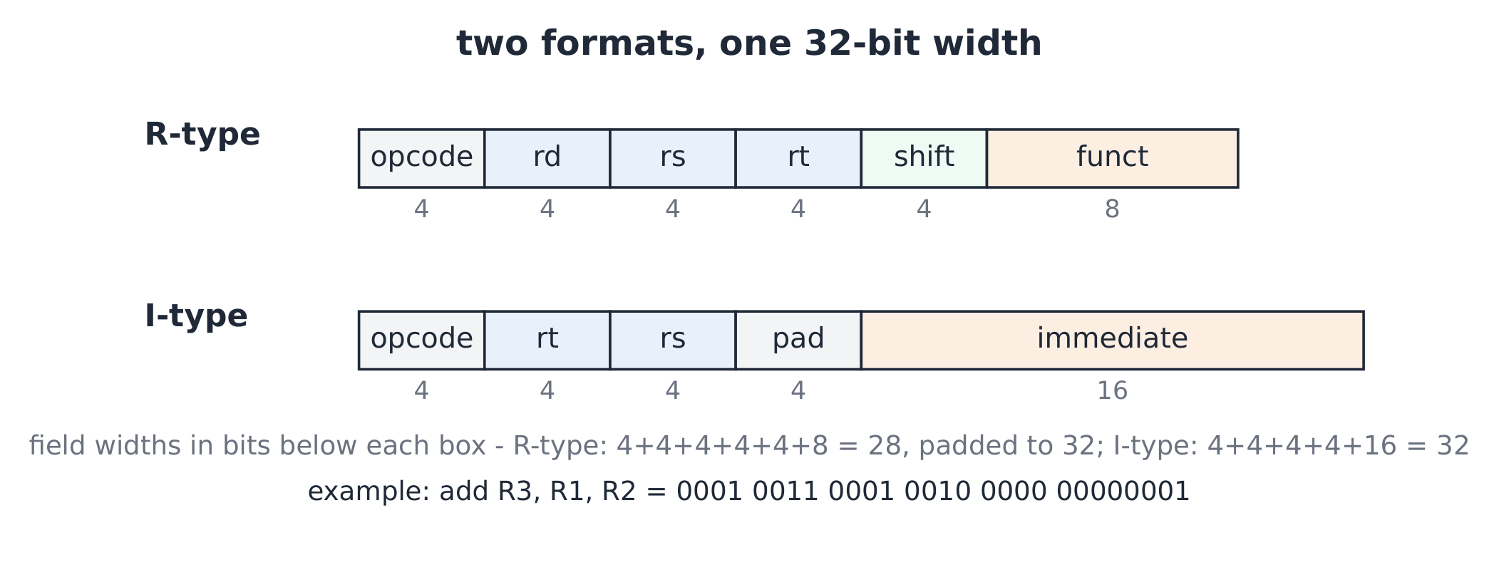
always zero. Two formats cover the course:
- R-type R 型:
opcode(4) | rd(4) | rs(4) | rt(4) | shift(4) | funct(8)— e.g.add rd, rs, rt. - I-type I 型:
opcode(4) | rt(4) | rs(4) | pad(4) | immediate(16)— e.g.lw rt, imm(rs); the pad field is unused, keeping the word 32 bits.
The derivation (the immediate's price). A 16-bit two's
complement immediate spans $-2^{15}$ to $2^{15} - 1$, i.e.
$-32\,768$ to $32\,767$ — so addi R2, R0, 40000 cannot encode and
the assembler demands two instructions (lui-style high half, then
add). Word addressing: with byte-addressable 字节寻址 memory and
32-bit words, lw offsets are multiples of $4$ — a 16-bit offset
reaches $2^{16}$ bytes = $64$ KiB from the base register.
Worked example 1 — encode and decode. Fields: opcode add = 1,
addi = 2, lw = 3, sw = 4, beq = 5. Encode add R3, R1, R2:
opcode $0001$, rd $0011$, rs $0001$, rt $0010$, shift $0000$, funct
$00000001$ — six fields, 28 of 32 bits used, the top 4 bits of the
final word zero-padded. Decode
0010 0100 0001 0000 000001111111 (opcode 2, rt = 4, rs = 1, pad =
0, immediate $01111111_2 = 127$): addi R4, R1, 127.
Worked example 2 — what R0 buys. addi R0, R0, 0 is the
canonical no-op; add R5, R0, R0 zeroes R5 in one cycle; comparing to
zero (beq R1, R0, loop) needs no constant operand. A dedicated zero
register removes a whole class of immediate-move instructions — CISC
kept MOV reg, 0; RISC keeps a wire.
Common mistakes. Reading a 16-bit immediate as unsigned (branch
and offset arithmetic is signed). Expecting add to touch memory
(load-store: it cannot). Assuming opcode alone selects the operation
(R-type also needs the funct field).
Summary. ISA = the stable contract; fixed-width R/I formats; 16-bit signed immediates reach $\pm 32$ K and 64 KiB of memory; R0 is a wire, not a register you write.
Datapath and control
Why it matters. The ISA is promises; the datapath 数据通路 is the plumbing that keeps them — and control 控制器 is the switch settings per instruction.
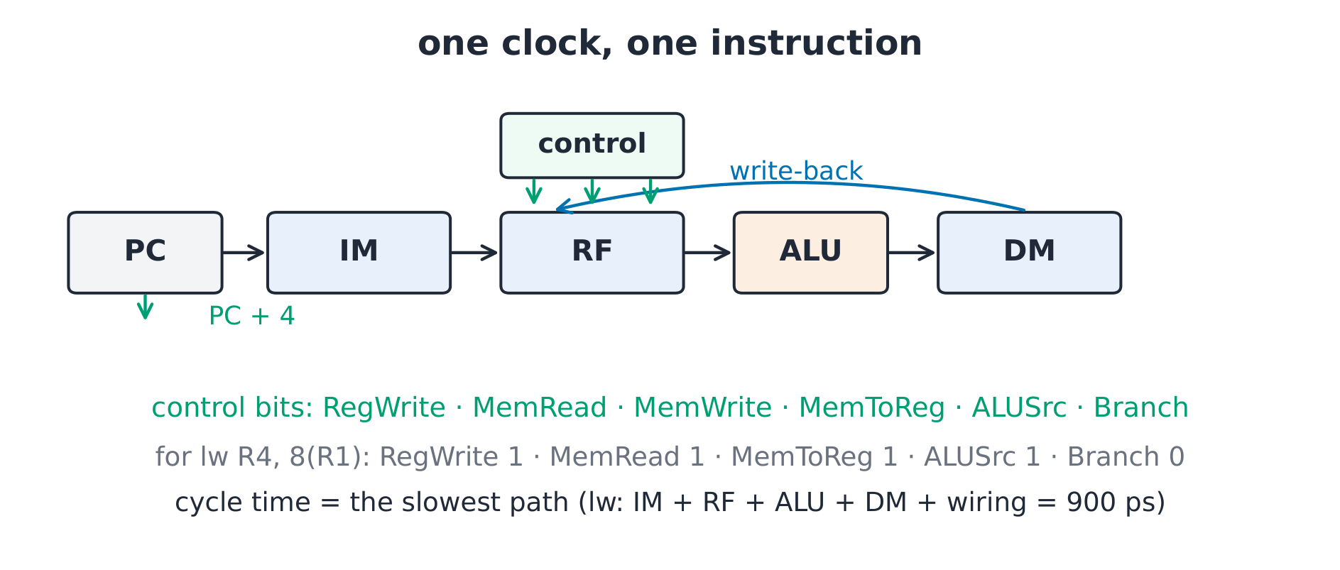
The idea, with a picture. The single-cycle machine: PC feeds the instruction memory (IM); register file (RF) reads two source registers; the ALU 算术逻辑单元 computes; data memory (DM) reads or writes; the result writes back; PC + 4 or a branch target loads the PC. Control sets: RegWrite, MemRead, MemWrite, MemToReg, ALUSrc, Branch.
The derivation (cycle time = the slowest path). All work happens
within one clock, so the clock must wait for the longest instruction:
memory read + register read + ALU + memory again + write back —
lw's path. With our parameters (IM 200 ps, RF read 100 ps, ALU 200
ps, DM 250 ps, wiring $150$ ps total; register writes overlap the
cycle's trailing edge): the lw path
$= 200 + 100 + 200 + 250 + 150 = 900$ ps, so the cycle is $900$ ps
and a 100-instruction program takes $90\,000$ ps. Speeding up add
would not help — the machine runs at its slowest citizen.
Worked example 1 — signals for one load. lw R4, 8(R1):
RegWrite = 1 (write R4), MemRead = 1, MemToReg = 1 (data memory to
register), ALUSrc = 1 (immediate for the address sum), Branch = 0,
MemWrite = 0. Six bits tell the whole story — the same datapath
executes every instruction; only the settings differ.
Worked example 2 — the store's exception. sw R5, 12(R1): the
write port goes to memory, not the register file: RegWrite = 0,
MemWrite = 1, MemRead = 0, MemToReg = x (don't care — nothing writes
back). Don't-care settings are a designer's freedom: whatever the
bit, the instruction behaves identically.
Common mistakes. Forgetting PC + 4 happens even on branches (the target is computed from PC + 4). Mixing MemToReg polarity between designs. Believing control is sequential — it is pure combinational logic on the opcode and funct.
Summary. One shared datapath, per-instruction control bits; the
cycle time is the slowest instruction's path; lw usually sets it.
Pipelining
Why it matters. The single-cycle machine idles most of its parts most of the time. Pipelining 流水线 overlaps instructions like an assembly line — more instructions finished per second, at almost the same hardware cost.
The idea, with a picture. Five stages: IF fetch, ID decode/register read, EX execute, MEM memory, WB write back. Instruction $i+1$ fetches while $i$ decodes: after the pipe fills, one instruction retires 完成 per cycle.
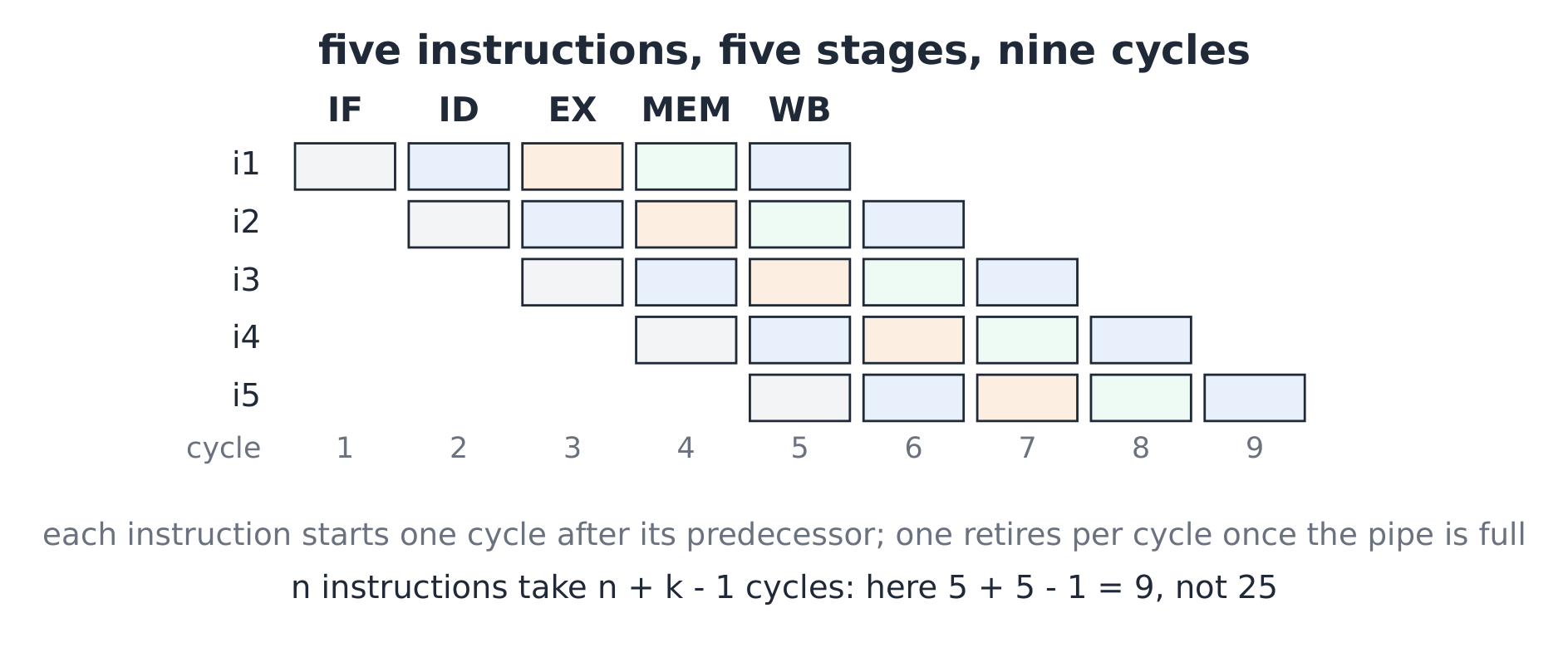
The derivation (the speedup formula). $n$ instructions, $k$ stages, stage time $t$: unpipelined time $= n k t$; pipelined $= (n + k - 1) t$ (fill $k - 1$, then one per cycle). Five instructions, five stages: $25t$ becomes $9t$; at $n = 100$: $500t$ becomes $104t$ — the speedup approaches $k$ as $n$ grows, and the ideal CPI 每条指令周期数 is $1$. Our stage time is set by the slowest stage: with IF 250, ID 150, EX 200, MEM 250, WB 100 ps, every stage costs $250$ ps — the pipeline runs at $250$ ps per instruction against the single cycle's $900$ ps.
Worked example 1 — a RAW hazard.
add R1, R2, R3     # R1 written in WB (cycle 6)
sub R4, R1, R1     # needs R1 in ID (cycle 5) — too early
The sub reads the register file one cycle before add writes it — a
read-after-write hazard 读后写相关. Forwarding 前递 routes the
ALU output of add straight back into the ALU inputs of sub, hiding
the wait entirely — except when the producer is a load: lw R1, …; add R3, R1, R2 must still stall one cycle, because the data
exists only after MEM.
Worked example 2 — CPI with stalls. A program runs $1000$ instructions on a 5-stage pipe with forwarding; $25\%$ are loads and half of those are followed immediately by a use (a load-use pair), each costing one stall: stalls $= 1000 \times 0.25 \times 0.5 = 125$. Total cycles $= 1000 + 125 + 4 = 1129$; CPI $= 1129 / 1000 = 1.129$ — the fill cost ($4$ cycles) fades as $n$ grows.
Common mistakes. Adding stage counts instead of using $n + k - 1$. Assuming forwarding fixes load-use (one bubble remains). Forgetting branches change PC late — a taken branch already fetched the wrong next instruction (our design: 1 bubble, resolved in EX).
Summary. $n + k - 1$ cycles for $n$ instructions; ideal CPI 1; forwarding kills ALU hazards, load-use costs one stall, taken branches cost one bubble; speedup tends to the stage count.
Memory hierarchy
Why it matters. The core wants bytes in nanoseconds; cheap memory answers in hundreds. The memory hierarchy 存储层次结构 stacks small-fast over big-slow and lets locality 局部性 pay the bills.
The idea, with a picture. A direct-mapped cache 直接映射缓存 places each memory block in exactly one slot: a 32-bit address splits into tag 标记 | index 索引 | offset 块内偏移. Our course cache: $4$ KiB, $16$-byte lines $\Rightarrow 256$ lines $\Rightarrow$ offset $4$ bits, index $8$ bits, tag $32 - 12 = 20$ bits.
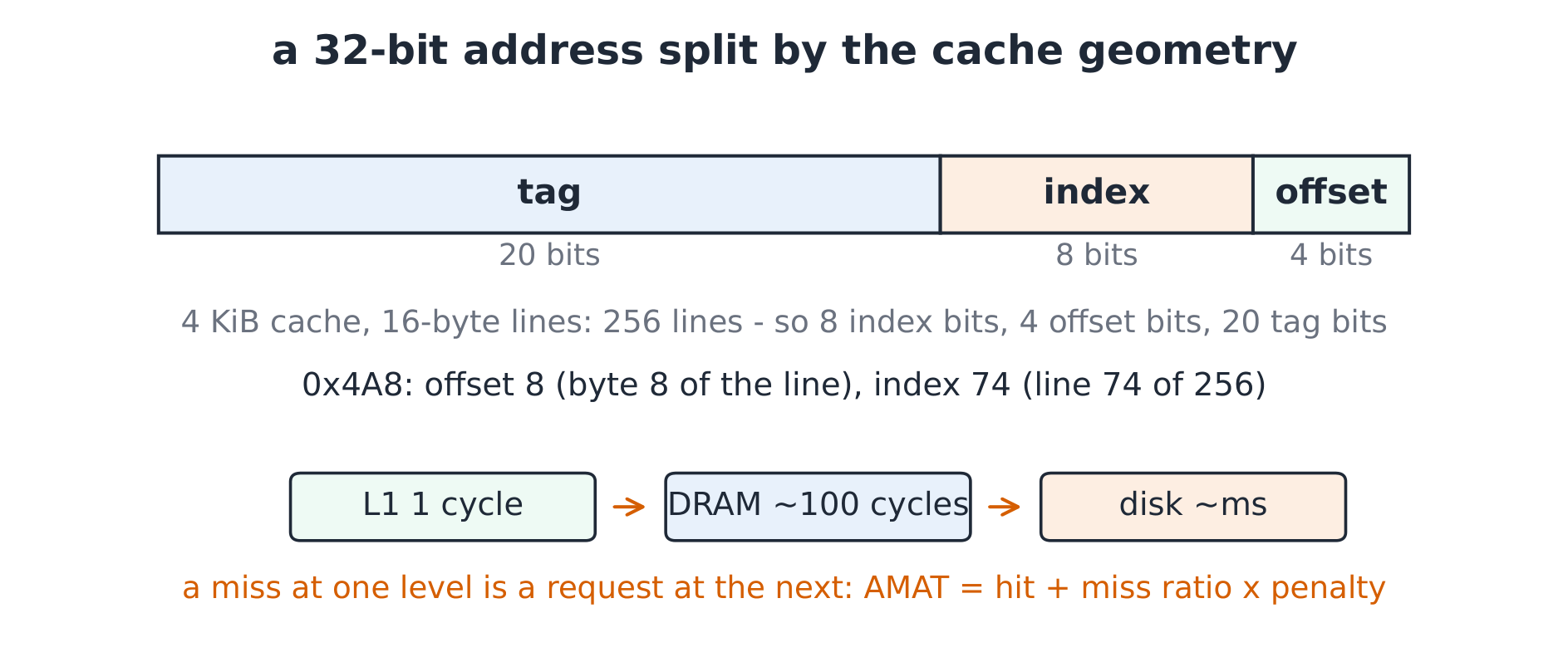
The derivation (AMAT). Average memory access time 平均访存时间 $= t_{\text{hit}} + p_{\text{miss}} \times t_{\text{penalty}}$. With L1 hit $1$ cycle, miss ratio $2\%$, penalty $100$ cycles: AMAT $= 1 + 0.02 \times 100 = 3$ cycles — a $3\times$ slowdown from a $2\%$ miss rate, which is why the hierarchy lives or dies on locality. Halve the miss ratio to $1\%$ and AMAT $= 2$: the sensitivity is linear in misses, not in hits.
Worked example 1 — where does an address go? Address $0x000004A8$: the low 12 bits are $0100\,1010\,1000$ — offset $1000_2 = 8$ (byte 8 of its line), index $0100\,1010_2 = 74$ (line 74 of 256), tag = the top 20 bits. One candidate line per address: any other block mapping to line 74 evicts 驱逐 it — direct-mapped's speed is one comparator, its price is conflict misses.
Worked example 2 — spatial and temporal locality. Row-major scanning of a $64 \times 64$ int array with 16-byte lines ($4$ ints per line): the first access misses, the next three hit — miss rate $1/4 = 25\%$ plus compulsory misses only; stride-16 access (one int per line, column-wise on a wide matrix) misses every access — $100\%$. Same array, same cache, four-times the AMAT: layout is a performance feature.
Common mistakes. Computing the index width from the cache size without dividing by the line size (it counts lines, not bytes). Expecting a bigger cache to fix a bad stride (bandwidth still moves one line at a time). Confusing miss rate with miss ratio (per-access versus per-instruction wording differs by the access count).
Summary. Split the address by geometry (tag | index | offset); AMAT $= 1 + m \times p$; direct-mapped trades conflicts for speed; locality — reuse and adjacency — is the currency.
Input/output
Why it matters. A machine that cannot talk is a space heater. I/O is where microseconds meet milliseconds, and the three transfer styles trade CPU attention for throughput.
The idea, with a picture. Programmed I/O 程序控制 I/O (polling): the core spins on a status register. Interrupt-driven I/O 中断驱动 I/O: the device signals, the core saves state and runs a handler. DMA 直接存储器访问: a DMA engine moves the block and interrupts once at the end.
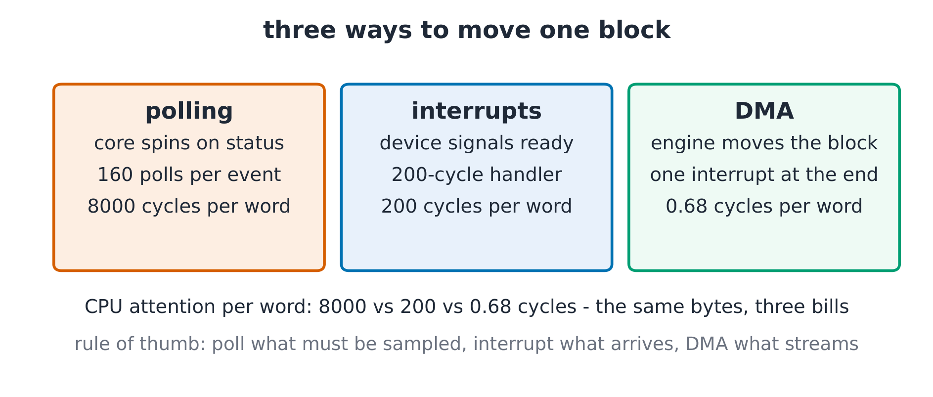
The derivation (the polling cost). A device flag updates every $2$ µs; one poll costs $50$ cycles at $250$ ps per cycle $= 12.5$ ns. Worst-case latency demands continuous polling: $2\,\mathrm{µs} / 12.5\,\mathrm{ns} = 160$ polls per event, all but one wasted — the core spends $160 \times 50 = 8\,000$ cycles per word of attention. Interrupts cut that to the handler cost: $200$ cycles of save, read, restore per word. DMA moves $1024$ words with one $500$-cycle setup plus one $200$-cycle completion interrupt: $0.68$ cycles per word against $200$ — three orders of magnitude of CPU attention saved.
Worked example 1 — choose the style. A keyboard (a human types $\approx 5$ characters per second): polling at that rate wastes the whole core; interrupts fit — one event per keypress, $200$ cycles each, negligible. A $4$ MiB disk block at $2$ GB/s: even interrupt-per-word drowns the core; DMA owns it. A sensor sampled exactly every $2$ µs: polling in a tight loop is honest and simple — the sample rate is the polling rate.
Worked example 2 — the interrupt bill. Each interrupt costs $200$ cycles of overhead (state save, vector, restore). Receiving $1024$ words one interrupt per word: $204\,800$ cycles of pure overhead; the same block by DMA: $700$ cycles total — the data moved identically, the CPU bill differs by $292\times$. Batching is not an optimization; it is the difference between architectures.
Common mistakes. Polling inside an interrupt handler (inverting the two styles). Forgetting DMA still needs cache coherence care (the DMA engine and the core both see memory). Confusing interrupt latency (time to start the handler) with throughput (words per second).
Summary. Polling: simple, core-hostile. Interrupts: event-priced, handler-overhead-per-word. DMA: block-priced, one interrupt per block — and the CPU attention per word falls by orders of magnitude.
Parallelism and performance
Why it matters. Clocks stopped getting faster; the machine got wider and more numerous instead. Reading a speedup now means reading Amdahl.
The idea, with a picture. A program has a serial fraction and a parallelizable fraction $f$. On $p$ processors: $\text{Speedup} = \dfrac{1}{(1 - f) + f / p}$ — the serial part never shrinks.
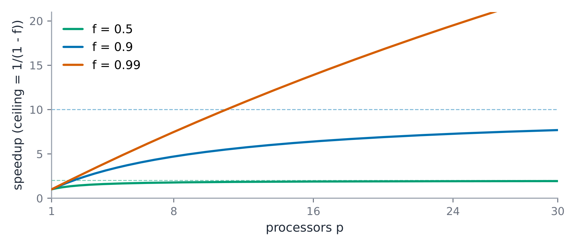
The derivation (the ceiling). As $p \to \infty$, speedup $\to 1 / (1 - f)$ — the serial fraction alone. With $f = 0.9$: unbounded hardware buys at most $10\times$; at $p = 8$: $1 / (0.1 + 0.1125) = 4.71\times$; at $p = 16$: $1 / (0.1 + 0.0563) = 6.40\times$ — the second eight processors add $1.7\times$ where the first eight added $4.7\times$. With $f = 0.99$ the ceiling is $100\times$, but reaching $50\times$ needs $p = 99$: $1/(0.01 + 0.99/99) = 50.0$ exactly. Diminishing returns are structural, not incidental.
Worked example 1 — price a speedup. A render spends $36$ s compositing (serial) and $64$ s shading (parallel) on one core: $f = 64/100 = 0.64$. On $p = 4$: speedup $= 1/(0.36 + 0.16) = 1.92\times$; runtime $= 100 \times 0.52 = 52.0$ s. Doubling the cores to $8$: $1/(0.36 + 0.08) = 2.27\times$, $44.0$ s — the compositing tail now dominates. The next purchase is an algorithm, not a machine.
Worked example 2 — instruction-level parallelism. Before cores, the pipeline itself is parallelism: the 5-stage machine overlaps five instructions (ILP 指令级并行). Adding hardware threads (SMT 同时多线程) lets one core fill pipeline bubbles with another thread's instructions — the hazard math of 6.3 still applies per thread. The stack: ILP within a core, threads per core, cores per chip — three levels, one Amdahl discipline.
Common mistakes. Reporting peak instead of measured speedup (nominal $p$ assumes $f = 1$). Treating a $10\%$ serial fraction as harmless — it caps every machine you will ever buy at $10\times$. Comparing speedups across different baselines (the single-core time must be the same program, same machine, one core active).
Summary. Speedup $= 1/((1-f) + f/p)$, ceiling $1/(1-f)$; serial fractions dominate at scale; ILP, threads and cores are one ladder — and the ladder leans on Amdahl.