What this course is, and how to use it
This is the second course in University Computer Science: discrete mathematics 离散数学 — the mathematics of objects you can list: statements, sets, graphs, counts. It is the proof toolkit behind algorithms, databases and every correct-by-construction claim in CS.
Scope limit, stated once: a study course, not a degree; every problem is original and self-contained, and every proof names its strategy.
- Units 2.1–2.3 are the proof engine: logic, sets, induction.
- Units 2.4–2.6 are the combinatorial engine: counting, graphs, discrete probability.
The discrete habit: name the strategy before the proof — direct, contraposition, contradiction, induction — and every identity is something you can verify on a small example first.
Logic and proofs
Why it matters. Logic is the type system of proof: translate the claim, check the argument, and choose the proof shape before writing a line.
The idea, with a picture. Propositions connect with ¬, ∧, ∨, →, ↔; a truth table 真值表 settles any formula over its variables ✓. The key equivalences: $p \to q \equiv \neg p \lor q$; contraposition $p \to q \equiv \neg q \to \neg p$; De Morgan $\neg(p \land q) \equiv \neg p \lor \neg q$ ✓. Predicate logic 谓词逻辑 adds the quantifiers $\forall x\, P(x)$ and $\exists x\, P(x)$, with negation flipping each.
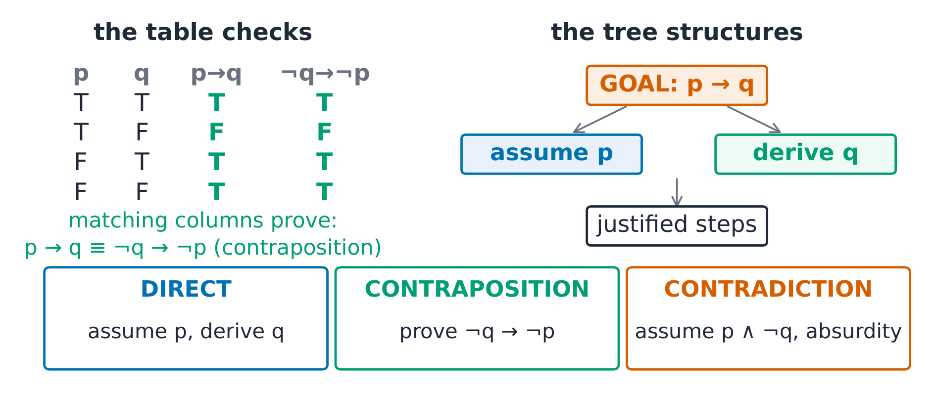
The derivation (why three proof shapes). To prove $p \to q$: direct proof 直接证明 (assume $p$, derive $q$); contraposition 逆否证明 (prove $\neg q \to \neg p$ — useful when negatives are friendlier); contradiction 反证法 (assume $p \land \neg q$, derive the impossible) ✓. Each shape converts the goal into an assumption you can compute with — choosing the shape is choosing your data.
Worked example 1 — the translation. Claim: every email has exactly one address: $\forall e\,\exists! a\,\text{Has}(e, a)$. Its negation pushes $\forall$ to $\exists$ and negates what follows: some email has no address, or has two or more ✓. One such email breaks the claim. Translate, negate, re-read: the three-step habit.
Worked example 2 — the strategy named. Claim: if $n^2$ is even then $n$ is even. Strategy: contraposition (the negative is friendlier). Proof: suppose $n$ odd, so $n = 2k+1$; then $n^2 = 4k^2 + 4k + 1 = 2(2k^2 + 2k) + 1$, odd ✓ — contrapositive proved, hence the claim.
Common mistakes. Proving the converse of what was asked (direction matters: $p \to q$ is not $q \to p$). Distributing negation without flipping connectives (De Morgan flips ∧ to ∨). Writing examples where a universal proof is demanded — an example is a check, not a proof.
Summary. Translate → choose shape (direct / contraposition / contradiction) → write justified steps; $p \to q \equiv \neg p \lor q$; De Morgan flips; negation swaps $\forall/\exists$; truth tables verify, proof trees structure.
Sets, functions and relations
Why it matters. Sets are the data model of discrete maths; functions are the typed pipes between them; relations carry the structure databases and graphs are built from.
The idea, with a picture. Operations: union, intersection, difference, complement; power set 幂集 $\mathcal{P}(A)$ = all subsets, $|\mathcal{P}(A)| = 2^{|A|}$ ✓. Functions classified by arrows: injective 单射 (no two inputs share an output), surjective 满射 (every output is hit), bijective 双射 (both — a perfect pairing) ✓. Composition $g \circ f$ applies $f$ then $g$; bijections invert.
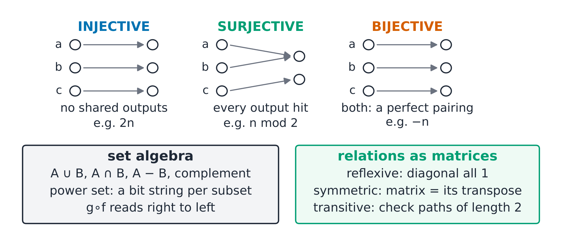
The derivation (why bijections count). A bijection pairs every element of $A$ with exactly one of $B$, so $|A| = |B|$ when one exists — and finding a bijection IS a counting proof ✓. That is why the number of subsets of an $n$-set pairs with bit strings of length $n$ (each element in or out — one bit each), proving $2^n$ without listing ✓.
Worked example 1 — classify three arrow diagrams. $f: \mathbb{Z} \to \mathbb{Z}$ by $f(n) = 2n$: injective (different inputs → different doubles) not surjective (odd numbers unhit) ✓; $g(n) = \lfloor n/2 \rfloor$: surjective not injective ✓; $h(n) = -n$: bijective — its own inverse ✓.
Worked example 2 — the relation test. On $\{1,2,3\}$: $R = \{(1,1), (2,2),(3,3),(1,2),(2,1)\}$ — reflexive (all loops), symmetric (edges come in pairs) and transitive — the chain $(1,2),(2,1)$ demands $(1,1)$ and the chain $(2,1),(1,2)$ demands $(2,2)$, both present ✓. So $R$ is an equivalence relation 等价关系 with classes $\{1,2\}$ and $\{3\}$ — check each property against the definition, not intuition.
Common mistakes. Confusing $\in$ (member) with $\subseteq$ (subset). Writing $f \circ g$ for $g \circ f$ (composition reads right-to-left). Testing symmetry by looking at one pair instead of all.
Summary. Union/intersection/difference/complement; $|\mathcal{P}(A)| = 2^{|A|}$ (bijection with bit strings); injective/surjective/bijective by arrows; composition right-to-left; relation properties — reflexive, symmetric, antisymmetric, transitive — tested against definitions.
Induction and recursion
Why it matters. Induction is the correctness proof of every loop and every recursive data structure; recursion is induction run backwards.
The idea, with a picture. To prove $\forall n \ge n_0\; P(n)$: base case 基础情形 ($P(n_0)$) + inductive step 归纳步骤 (assume $P(k)$ — the induction hypothesis 归纳假设 — derive $P(k+1)$) ✓. Recursion defines $F$ by smaller calls: factorial $0! = 1$, $n! = n \cdot (n-1)!$ — the same ladder, built instead of climbed.
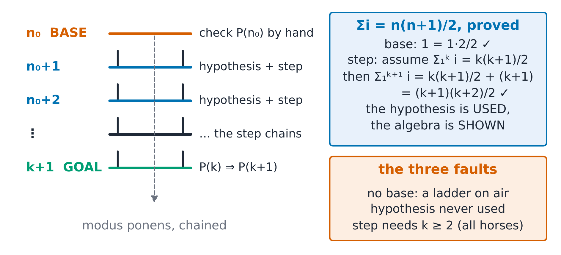
The derivation (why induction is valid). The step proves that if rung $k$ holds then rung $k+1$ holds; the base proves rung $n_0$; chaining gives every rung up to any $n$ — induction is repeated modus ponens ✓. Fault detection: no base (a ladder on air), hypothesis not invoked (a step that proves nothing), or step from $k$ assuming more than $P(k)$.
Worked example 1 — the sum identity. Claim: $\sum_{i=1}^{n} i = \frac{n(n+1)}{2}$. Strategy: induction. Base $n=1$: $1 = \frac{1 \cdot 2}{2}$ ✓. Step: assume $\sum_{i=1}^{k} i = \frac{k(k+1)}{2}$; then $\sum_{i=1}^{k+1} i = \frac{k(k+1)}{2} + (k+1) = \frac{(k+1)(k+2)}{2}$ ✓ — the hypothesis is used, the algebra is shown, the claim closes.
Worked example 2 — the faulty proof caught. The claim that all horses are the same colour: base trivially true; the step — remove one horse from each side — fails at $k+1 = 2$ because the two overlapping sets share no horse ✓ — the step must hold for EVERY $k$, including the smallest; a step that silently needs $k \ge 2$ without base $P(2)$ is the classic fault.
Common mistakes. Omitting the base — hypothesis plus step prove nothing without a floor. Using $P(k+1)$ to prove $P(k+1)$ (circular). Strong induction declared but ordinary step written — say which and do which.
Summary. Base + hypothesis + step, hypothesis explicitly invoked; strong induction assumes all rungs below; recursion = induction's mirror (defined downwards); faults: missing base, unused hypothesis, step valid only for large $k$.
Counting and combinatorics
Why it matters. Counting is complexity analysis's arithmetic: sizes of state spaces, branch counts, the how-many behind every loop bound.
The idea, with a picture. Addition rule 加法原理: disjoint choices add; multiplication rule 乘法原理: sequential choices multiply ✓. Permutations 排列 (ordered): $P(n, r) = \frac{n!}{(n-r)!}$; combinations 组合 (unordered): $\binom{n}{r} = \frac{n!}{r!\,(n-r)!}$ ✓. Inclusion–exclusion 容斥原理: $|A \cup B| = |A| + |B| - |A \cap B|$ — add, then subtract the double count.
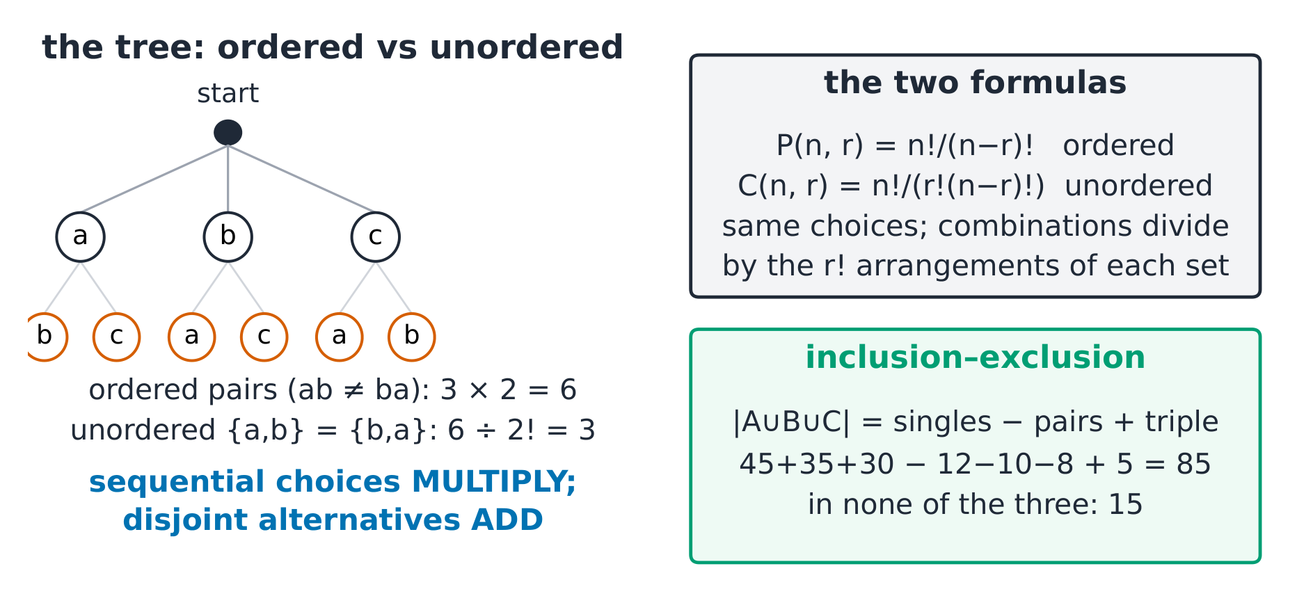
The derivation (why the formulas divide). Permutations choose and arrange: $n$ options, then $n-1$, …, $r$ factors — multiply. Combinations identify arrangements of the same $r$ objects: every set of $r$ was counted $r!$ times as an arrangement — divide by $r!$ ✓. The division is the entire difference between ordered and unordered.
Worked example 1 — the committee. A team of 3 from 8 people, with one designated leader: choose the team $\binom{8}{3} = 56$, pick the leader among them 3 ways → $168$ ✓; or choose the leader first (8) then 2 members from 7 ($\binom{7}{2} = 21$) → $168$ — two counting routes, one answer, and the agreement is the check.
Worked example 2 — inclusion–exclusion with three sets. Among 100 students: 45 like tea, 35 coffee, 30 cocoa; 12 tea∧coffee, 10 tea∧cocoa, 8 coffee∧cocoa; 5 all three. At least one: $45+35+30-12-10-8+5 = 85$ ✓ — none: $100 - 85 = 15$. Add singles, subtract pairs, add the triple: each element counted once.
Common mistakes. Adding where choices are sequential (routes × vehicles multiply). Using permutations where order is irrelevant (committees are combinations). Applying two-set inclusion–exclusion to three sets (the triple comes back with a plus).
Summary. Disjoint → add; sequential → multiply; $P(n,r)$ ordered, $\binom{n}{r} = P/r!$ unordered; inclusion–exclusion: + singles − pairs
- triples; count two ways and compare — the checksum of combinatorics.
Graphs and trees
Why it matters. Graphs are the universal model — networks, states, dependencies; trees are the workhorse of search and storage; and the handshake lemma 握手引理 is the first must-hold identity of the course.
The idea, with a picture. $G = (V, E)$; representations: adjacency matrix 邻接矩阵 ($n^2$ space, $O(1)$ edge test), adjacency list 邻接表 ($O(|V|+|E|)$) ✓. Tree 树: connected, acyclic, $|E| = |V| - 1$ ✓. Traversals: BFS 广度优先搜索 (queue, level order, shortest paths in unweighted graphs), DFS 深度优先搜索 (stack/recursion, component discovery).
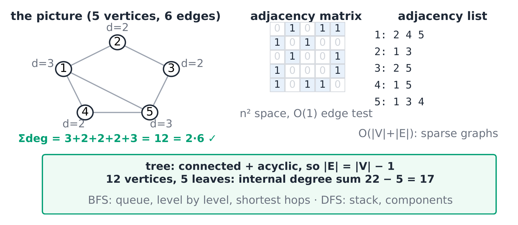
The derivation (why handshaking must hold). Each edge contributes 1 to the degree of each endpoint, so every edge adds exactly 2 to the degree sum: $\sum_{v} \deg(v) = 2|E|$ ✓ — immediate corollaries: the number of odd-degree vertices is even; a graph where all $n \ge 2$ vertices have distinct degrees cannot exist (degrees run $0..n-1$ but 0 and $n-1$ cannot coexist) ✓.
Worked example 1 — the model choice. (Design question) social friendships (undirected, adjacency list — sparse), task dependencies (directed acyclic, matrix when small — cycle tests), city metro (weighted, Dijkstra's queue — beyond scope, named as such) ✓ — the problem's symmetry dictates the graph, the density dictates the representation.
Worked example 2 — tree arithmetic. A tree has 12 vertices of which 5 are leaves (degree 1): with $|E| = 11$ and handshake, the internal 7 vertices carry degree sum $22 - 5 = 17$ ✓ — every tree question is a walk over $|E| = |V| - 1$ plus $\sum \deg = 2|E|$.
Common mistakes. Forgetting degree 0 counts (isolated vertices are vertices). Confusing connected (one piece) with complete (all edges). Assuming BFS gives shortest paths in weighted graphs (it does not — that needs weighted methods).
Summary. $G = (V,E)$; matrix vs list by density; tree: connected + acyclic + $|E| = |V|-1$; BFS level order / DFS component order; $\sum \deg = 2|E|$, odd-degree count even; choose the model from the problem's symmetry.
Discrete probability
Why it matters. Randomised algorithms, average-case analysis and hashing all run on exact discrete probability — the same counting from 2.4, now over equally likely outcomes.
The idea, with a picture. A sample space 样本空间 $\Omega$ of equally likely outcomes; events are subsets; $P(E) = |E|/|\Omega|$ ✓. Conditional probability 条件概率 $P(A \mid B) = \frac{P(A \cap B)}{P(B)}$; Bayes' theorem 贝叶斯定理 $P(A \mid B) = \frac{P(B \mid A) P(A)} {P(B)}$ ✓; independence $P(A \cap B) = P(A)P(B)$.
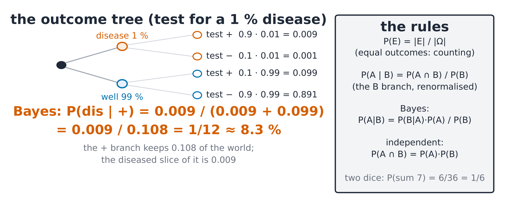
The derivation (why conditioning shrinks the world). Conditioning on $B$ keeps only the $B$-outcomes and renormalises their weights to sum to 1 — the fraction of $B$-world where $A$ also holds ✓. That is the entire numerator/denominator of Bayes: $P(B \mid A)P(A)$ sizes the $A \cap B$ slice; $P(B)$ rescales to the $B$-world.
Worked example 1 — dice by counting. Two fair dice: $\Omega$ has 36 pairs. $P(\text{sum} = 7) = 6/36 = 1/6$ (six pairs); $P(\text{sum} = 11) = 2/36$ ✓; $P(\text{sum} = 7 \text{ or } 11) = 8/36 = 2/9$ — counting from 2.4 does all the work.
Worked example 2 — Bayes on a test. A disease affects 1 %; a test has sensitivity 90 % and specificity 90 %. $P(\text{dis} \mid +) = \frac{0.9 \times 0.01}{0.9 \times 0.01 + 0.1 \times 0.99} = \frac{0.009} {0.108} = 1/12 \approx 8.3\ \%$ ✓ — the same arithmetic as MED12 §4, derived here from the tree: rare conditions stay improbable after imperfect evidence.
Common mistakes. Adding conditional probabilities as if independent (the conditioning world must be one world). Confusing $P(A \mid B)$ with $P(B \mid A)$ (the prosecutor's fallacy). Counting outcomes of different likelihood as equal (only equally likely outcomes give $|E|/|\Omega|$).
Summary. $P = |E|/|\Omega|$ on equally likely outcomes; $P(A \mid B) = P(A \cap B)/P(B)$ — the B-branch renormalised; Bayes rescales slices between worlds; independence multiplies; dice, cards and hash tables are all counting problems underneath.