What this course is, and how to use it
This is the fifth course in University Computer Science: data structures and algorithms 数据结构与算法 — the containers a program reaches for and the recipes that walk them, chosen by what they cost.
Scope limit, stated once: a study course, not a degree; Python 3 is the vehicle, every fragment is original, and every cost claim in this handout was verified by counting operations on the exact datasets printed here.
- Units 5.1 is the yardstick: how cost grows.
- Units 5.2–5.5 are the containers: linear lists, hash tables, trees, graphs.
- Units 5.6–5.7 are the recipes: sorting and searching.
The measuring habit: never trust a cost claim you have not counted — each unit fixes a dataset, and the suite re-derives every number.
Asymptotic analysis
Why it matters. Choosing between two solutions is choosing between their growth rates: at $n = 1000$, the difference between $n \log n$ and $n^2$ is a factor of about $100$.
The idea, with a picture. Big-O 大O记号 is an upper bound up to a constant: $f(n) = O(g(n))$ when $f(n) \le c\,g(n)$ for large $n$. Big-Ω is the lower-bound twin, Big-Θ 大Θ记号 the exact rate. Drop constants and lower-order terms: $3n^2 + 5n + 7$ is $\Theta(n^2)$ — the $n^2$ term eats the rest as $n$ grows.
| $n$ | $\log_2 n$ | $n$ | $n\log_2 n$ | $n^2$ | $2^n$ |
|---|---|---|---|---|---|
| 10 | 3 | 10 | 33 | 100 | 1 024 |
| 100 | 7 | 100 | 664 | 10 000 | $\approx 10^{30}$ |
| 1000 | 10 | 1000 | 9 966 | $10^6$ | $\approx 10^{301}$ |
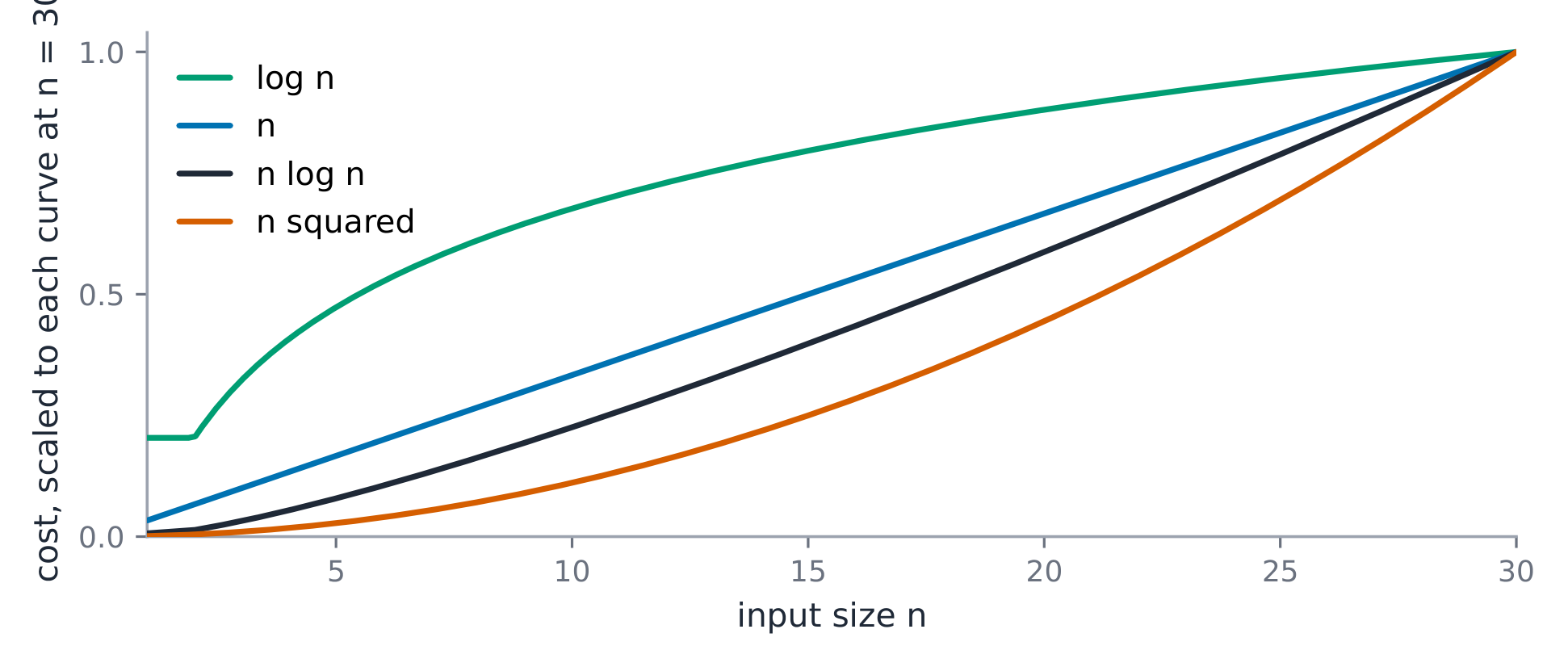
The derivation (why log n for halving). Each halving of the input leaves one step: an algorithm that halves $n$ every step touches $\log_2 n$ levels — binary search on $n = 16$ makes at most $4$ probes because $2^4 = 16$. And $\log$ of a million is about $20$: flatness is why log-time algorithms feel instant.
Worked example 1 — counting beats guessing. Two loops over the same array of $n = 100$ items: the single loop runs its body $100$ times; the nested one $100 \times 100 = 10\,000$ times. Double $n$ to $200$: the linear body doubles to $200$, the nested quadruples to $40\,000$ — the measured ratio $4 = 2^2$ is the exponent, read off the data.
Worked example 2 — reading code as a class. A loop that halves
i = i // 2: $\Theta(\log n)$ steps. Two sequential loops over $n$: the
costs add, $\Theta(n) + \Theta(n) = \Theta(n)$. A loop inside a halving
loop: they multiply, $\Theta(n \log n)$ — the shape of merge sort.
Common mistakes. Reading Big-O as a speed guarantee (constants matter at small $n$). Forgetting the input layout: $O(1)$ indexing is an array property, not a linked-list one. Reporting the best case where the worst case was asked.
Summary. O bounds above, Ω below, Θ pins the rate; drop constants and low-order terms; measure by doubling and read the exponent.
Lists, stacks and queues
Why it matters. The linear structures are the default containers, and their costs differ at the ends: knowing which end is cheap is the whole subject.
The idea, with a picture. A Python list is a contiguous array 数组: index $i$ computes an address, $O(1)$; inserting at the front moves everything, $O(n)$. A linked list 链表 trades the jump for cheap splices: each node 节点 carries a pointer to the next. A stack 栈 adds and removes at one end (LIFO); a queue 队列 adds at one end, removes at the other (FIFO).
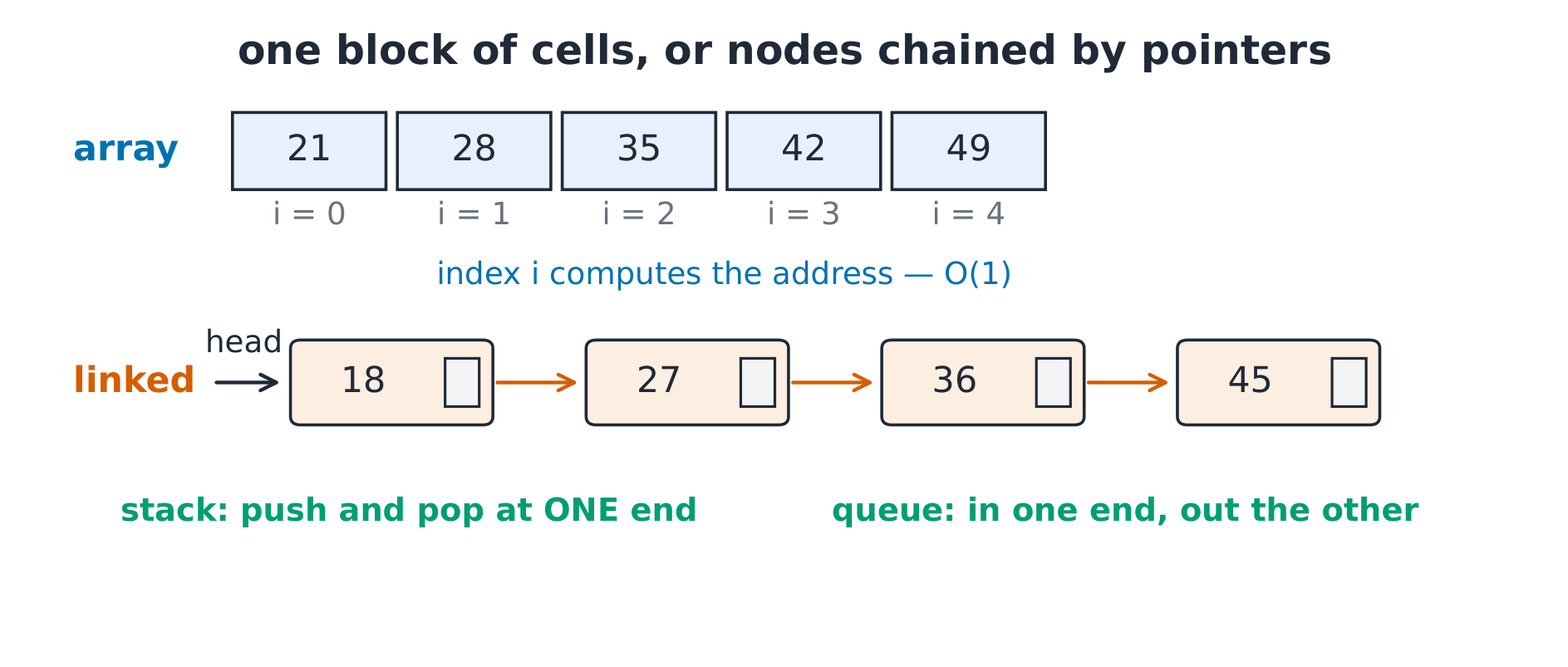
The derivation (why append is amortized O(1)). The array grows by doubling: appending $n$ items copies each element at most once in total across all regrows — total copies $\le 2n$ for $n$ appends, so the average append is constant even though one regrow copies $n$. Inserting at position $0$ never amortises: every call slides all $n$ residents, so $n$ front-inserts move $\Theta(n^2)$ elements (measured: the operation count quadruples when $n$ doubles).
Worked example 1 — a stack trace. push 3, push 7, push 1, then
pop, pop: the pops return $1$ then $7$ — last in, first out. The
classic use is balanced brackets: scan ([]){}, pushing opens;
each closer must match the top — the string is balanced, while ([)]
fails because ) finds [ on top.
Worked example 2 — a queue trace. Enqueue a, b, c; two dequeues
return a then b; the front is c. First in, first out. Two stacks
can fake a queue (inbox and outbox, each element handled twice), which
is why collections.deque — a doubly-ended list — serves both ends in
$O(1)$.
Common mistakes. Using list.pop(0) in a loop ($O(n)$ each; use
deque.popleft()). Searching a linked list by index (walk the chain,
$O(n)$). Assuming the Python list is linked — it is an array.
Summary. Array: $O(1)$ index, $O(n)$ front insert. Linked: $O(1)$ splice after a located node. Stack one end, queue two ends; deque does both ends in $O(1)$.
Hashing
Why it matters. A hash table is the structure that answers membership in one expected step — the engine inside sets, dictionaries and caches.
The idea, with a picture. A hash function 哈希函数 maps a key to a bucket: $h(k) = k \bmod 13$ sends $4, 17, 30, 43$ all to bucket $4$ — a collision 冲突. Chaining 链地址法 hangs a list off each bucket; open addressing 开放寻址法 walks to the next free slot (linear probing: $17 \to 5$, $30 \to 6$, $43 \to 7$).
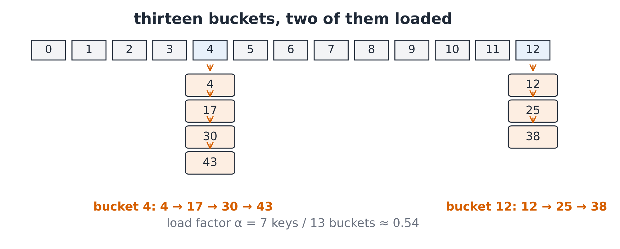
The derivation (the load factor rules the chain). With $m$ buckets and $n$ keys, the load factor 负载因子 $\alpha = n/m$ is also the average chain length: our fixed keys $[4, 17, 30, 43, 12, 25, 38]$ give $\alpha = 7/13 \approx 0.54$, with bucket $4$ holding $4$ keys, bucket $12$ holding $3$, and eleven buckets empty. Successful search costs about $1 + \alpha/2$ comparisons with chaining; grow $m$ with $n$ and the expected cost stays $O(1)$ — that resize is why dictionaries stay fast.
Worked example 1 — exact chains. Insert $4, 17, 30, 43$ with $h(k) = k \bmod 13$: every key hashes to $4$, so the chain reads $4 \to 17 \to 30 \to 43$. Searching $43$ walks $4, 17, 30, 43$: four comparisons — the worst case a table this loaded can produce, and exactly what the uniform hash avoids on average.
Worked example 2 — probing the same set. Open addressing with linear probing: $4$ lands in slot $4$; $17$ probes $4$ (taken) $\to 5$; $30$ probes $4, 5 \to 6$; $43$ probes $4, 5, 6 \to 7$. Total probes: $1 + 2 + 3 + 4 = 10$ for four insertions — clustering 聚集 grows the runs, which is why real tables keep $\alpha$ under about $0.75$ and why the probing order matters.
Common mistakes. Modulo a power of two when keys share low bits (pick a prime). Mutating a key while it sits in the table (its hash moves). Expecting $O(1)$ worst case — that guarantee needs a perfect hash or a tree bucket.
Summary. Hash spreads keys; collisions are normal, so pick the resolution (chain or probe); $\alpha = n/m$ predicts the cost; resize to keep it constant.
Trees and heaps
Why it matters. Trees buy logarithmic costs by splitting the remaining work in half at each level — search, insert and (for heaps) min/max in $O(\log n)$.
The idea, with a picture. A binary search tree 二叉搜索树 keeps the order invariant: left subtree $<$ node $<$ right subtree. Inserting $50, 30, 70, 20, 40, 60, 80$ builds a perfect tree of height $2$; the inorder walk reads $20, 30, 40, 50, 60, 70, 80$ — sorted, by construction. A heap 堆 is a complete tree stored in an array: children of index $i$ sit at $2i+1$ and $2i+2$; a min-heap 小顶堆 keeps every parent $\le$ its children, so the minimum lives at index $0$.
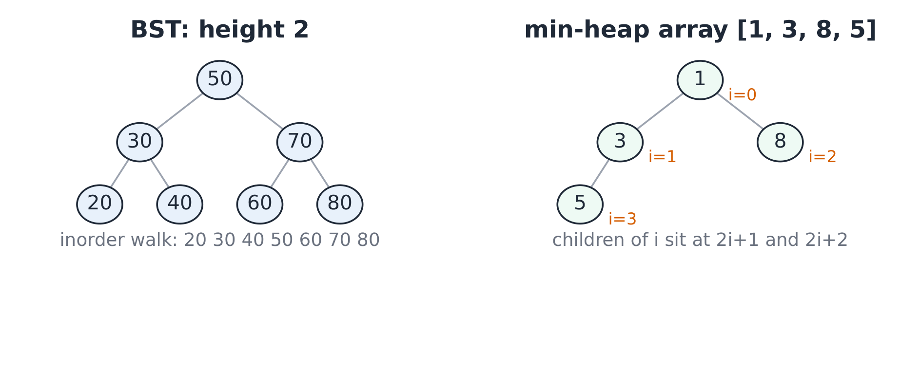
The derivation (height is the cost). A perfect tree of height $h$ holds $2^{h+1} - 1$ nodes: $7$ at $h = 2$, $15$ at $h = 3$, $31$ at $h = 4$ — so $n$ nodes need height $\lfloor \log_2 n \rfloor$ when balanced, and every root-to-leaf walk (search, insert, sift) pays that height. Skew breaks the deal: inserting sorted keys $1, 2, 3, 4$ makes a chain of height $3 = n - 1$ — $O(n)$ search, the reason balanced variants (AVL, red-black) rotate to stay logarithmic.
Worked example 1 — BST search and insert. Search $40$: compare $50$ (right is smaller keys — go left), $30$ (go right), $40$ — found in $3$ comparisons against $7$ nodes: the level count. Insert $35$: walk the same path, hang it left of $40$; the inorder walk now reads $20, 30, 35, 40, 50, 60, 70, 80$ — still sorted.
Worked example 2 — heap sift-ups. Build a min-heap by inserting
$5, 3, 8, 1$: $5$ lands at index $0$; $3$ sifts up over $5$; $8$ stays;
$1$ sifts up over $5$ then over $3$, landing at index $0$. The array
reads $[1, 3, 8, 5]$ — parent $\le$ child everywhere (check: $1 \le 3,
8$; $3 \le 5$). heapq.heapify builds the whole array in $O(n)$ by
sifting down from the middle.
Common mistakes. Forgetting the heap is only half-ordered (an inorder walk of $[1, 3, 8, 5]$ is meaningless; only the root is special). Expecting BST balance from random luck on sorted input. Storing a tree of $n$ nodes in $n+1$ array slots and off-by-one-ing the child formula.
Summary. BST: order invariant, inorder = sorted, cost = height, $\log$ when balanced. Heap: complete shape in an array, parent dominates children, root is the min in $O(1)$, sift costs the height.
Graphs and traversal
Why it matters. Every network — roads, prerequisites, friend-of-friend — is a graph, and the two traversals are the probes that answer reachability, layers and structure.
The idea, with a picture. A graph $G = (V, E)$: our fixed course graph has $V = \{A \ldots H\}$ ($8$ nodes) and $10$ undirected edges: $AB, AC, BD, CD, CE, DF, EF, EG, FH, GH$. The adjacency list 邻接表 stores, per node, its neighbours ($20$ entries for $10$ undirected edges); the adjacency matrix 邻接矩阵 is an $8 \times 8$ grid of $64$ cells, $1$ at an edge.
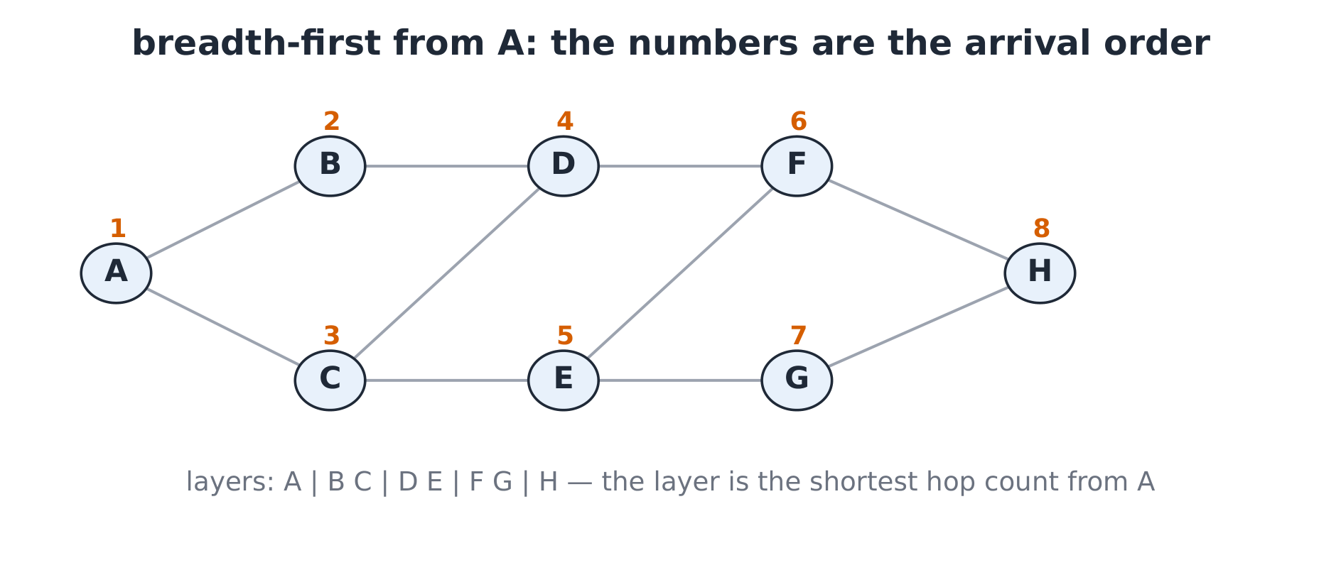
The derivation (why O(V+E)). Breadth- and depth-first search mark each node once ($V$ work) and scan each stored edge once ($E$ work): $O(V + E) = O(8 + 10)$ visits on the course graph. The matrix pays $O(V^2)$ because every row walks all $8$ columns, edge or not — the list wins on sparse graphs ($E \ll V^2$), the matrix wins when the graph is dense or the question is just one cell lookup.
Worked example 1 — BFS by layers. From $A$ with neighbours visited alphabetically: layer 0 is $A$; layer 1 is $B, C$; layer 2 is $D, E$; layer 3 is $F, G$; layer 4 is $H$. The full order reads $A, B, C, D, E, F, G, H$, and the layer of a node is its shortest unweighted distance from $A$ — that is what a queue buys: the frontier leaves in arrival order.
Worked example 2 — DFS by stack. From $A$, walking neighbours alphabetically: $A \to B \to D$; $D$'s next unvisited neighbour is $C$; $C \to E$; $E \to F$; $F \to H$; $H$'s unvisited neighbour $G$ closes the walk. The order reads $A, B, D, C, E, F, H, G$ — one deep walk that backtracks at dead ends. Same graph, same $O(V+E)$, different shape: BFS answers shortest hops, DFS exposes paths and cycles.
Common mistakes. Forgetting to mark visited (infinite loop on any cycle). Reading the BFS layer as weighted distance (unweighted only — weights need Dijkstra). Storing undirected edges once in a matrix (both cells $[u][v]$ and $[v][u]$ must be set).
Summary. List for sparse, matrix for dense; both traversals are $O(V+E)$; the queue gives layers and shortest hops, the stack gives deep paths.
Sorting
Why it matters. Sorting is the precondition for binary search, deduplication and merging — and the canonical lesson in cost analysis: same task, wildly different bills.
The idea, with a picture. The course dataset is $[5, 2, 9, 1, 7, 3]$. Insertion sort 插入排序 grows a sorted prefix, sliding each new card back: after the pass over $1$ the prefix reads $1, 2, 5, 9$. Merge sort 归并排序 halves, sorts each half, merges. Quicksort partitions around a pivot. Bubble sort swaps adjacent inversions — educational, rarely used.
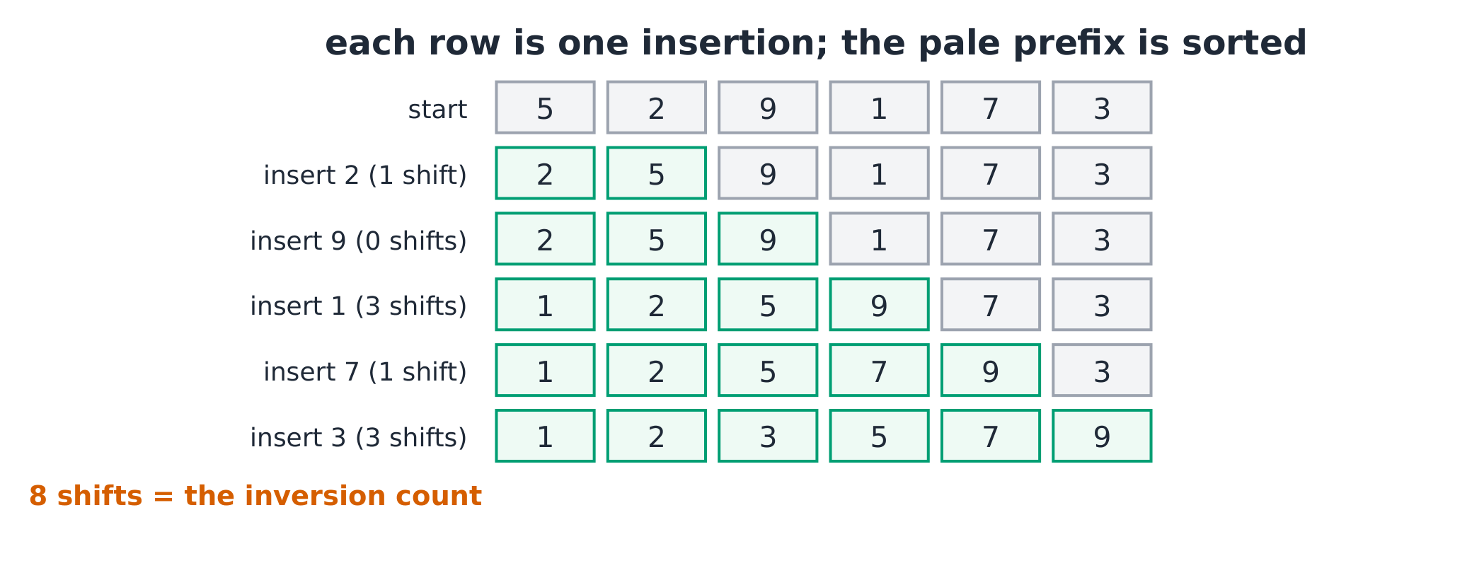
The derivation (the inversion count). An inversion 逆序 is a pair out of order. On the course dataset the inversions are $(5,2), (5,1), (5,3), (2,1), (9,1), (9,7), (9,3), (7,3)$ — eight pairs. Every adjacent swap fixes exactly one inversion, so any swap-adjacent sort makes exactly $8$ swaps here; insertion sort's shifts equal the inversions too. Merge sort counts the same inversions across its merges while moving each element at most $\log_2 6 \approx 2.6$ levels: $O(n \log n)$ beats $O(n^2)$ because it fixes many inversions per move.
Worked example 1 — insertion by hand. $[5, 2, 9, 1, 7, 3]$: insert $2$ (one shift: $5, 2 \to 2, 5$); $9$ appends (no shift); $1$ shifts three ($[1, 2, 5, 9]$); $7$ passes $9$ only (one shift, prefix $[1, 2, 5, 7, 9]$); $3$ shifts three. Total shifts $1 + 0 + 3 + 1 + 3 = 8$ — exactly the inversion count — with $11$ comparisons (each pass ends in one failed comparison), and the sorted result $[1, 2, 3, 5, 7, 9]$.
Worked example 2 — merge sort on the same data. Halve to $[5, 2, 9]$ and $[1, 7, 3]$; recursively $[2, 5, 9]$ and $[1, 3, 7]$; merge: $1, 2, 3, 5, 7, 9$. The measured comparison count is $10$ on this input, against insertion's $11$ — close here, but the families diverge: at $n = 1000$, $n \log_2 n \approx 9\,966$ against $n^2 = 10^6$, a factor of about $100$.
Common mistakes. Calling quicksort's worst case rare and forgetting sorted input with a first-element pivot IS the worst case ($O(n^2)$). Expecting heapsort to be stable (it is not; merge sort is). Counting only comparisons when moves dominate on large records.
Summary. Adjacent-swap sorts pay one move per inversion ($\Theta(n^2)$ worst); divide-and-conquer pays $\Theta(n \log n)$; stability survives in merge and insertion, not in quick or heap.
Searching
Why it matters. Membership and lookup are the most-run operations in real programs — the difference between $16$ probes and $4$ is the difference between linear and binary on a page of data.
The idea, with a picture. Linear search 线性查找 walks the array: $O(n)$, no preconditions. Binary search 二分查找 halves a sorted range: compare the middle, keep one half. On the sorted array of $16$ items $[3, 7, 11, 15, 19, 23, 27, 31, 35, 39, 43, 47, 51, 55, 59, 63]$ (indices $0$–$15$), searching $43$ probes indices $7, 11, 9, 10$ — value $31$, then $47$, then $39$, then $43$: four probes, found.
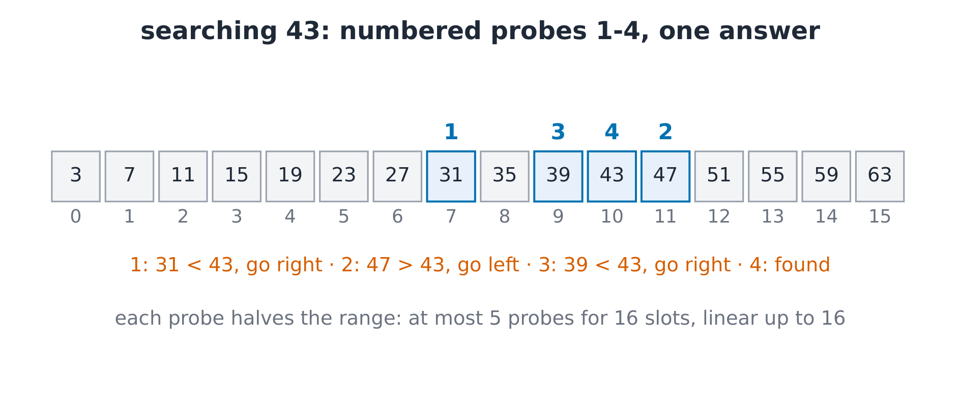
The derivation (the probe bound). Each probe halves the candidates: after $k$ probes at most $\lceil n / 2^k \rceil$ remain, so the worst case is $\lceil \log_2(n+1) \rceil$ probes — for $n = 16$ that is $5$ (and our hit took $4$). Linear pays $16$ at the far end and $16$ more for every miss beyond the end; binary pays the same $\le 5$ for every query. The precondition is the sort: on unsorted data the halving argument collapses, and only linear remains honest.
Worked example 1 — the probe trail. Searching $43$: $lo=0$, $hi=15$, $mid=7$ reads $31 < 43$ so $lo=8$; $mid=11$ reads $47 > 43$ so $hi=10$; $mid=9$ reads $39 < 43$ so $lo=10$; $mid=10$ reads $43$ — found at index $10$ after $4$ probes. Compare: linear walks $11$ values to reach index $10$.
Worked example 2 — the miss that proves the bound. Search $64$ (absent, above the end): binary probes $7 (31), 11 (47), 13 (55), 14 (59), 15 (63)$ — five probes, then the empty range reports absent. Linear would walk all $16$ and report the same absent — the miss costs binary its worst case and linear its full array, and the gap still grows with $\log$ versus $n$.
Common mistakes. Binary search on unsorted data (silently wrong
answers, not crashes). Off-by-one in the update (lo = mid instead of
mid + 1 loops forever). Computing mid as $(lo + hi) / 2$ in languages
with fixed-width overflow (lo + (hi - lo) // 2 is safe).
Summary. Linear: no precondition, $O(n)$. Binary: sorted precondition, $\lceil \log_2(n+1) \rceil$ probes worst case — $16$ slots resolve in at most $5$.