What this course is, and how to use it
This is the thirteenth course in University Computer Science: artificial intelligence and machine learning 人工智能与机器学习 — the classical core: search, reasoning, probability, learning from data, and the honesty apparatus (evaluation, leakage, fairness) that keeps it trustworthy.
Scope limit, stated once: a study course, not a degree; one documented synthetic dataset — Overnight, 200 fictional parcel-delivery records with a data card — supplies every computation, and every metric in this handout is recomputed by the suite from first principles.
- Units 13.1–13.3 are the classical spine: search, knowledge, probability.
- Units 13.4–13.5 learn from data: models and their optimisation.
- Units 13.6–13.7 keep them honest: evaluation, leakage, fairness.
The modelling habit: a number without a resampling story is an anecdote — every score in this course is recomputed.
Search
Why it matters. Search is problem solving as exploring a space of choices — routing, scheduling, game moves — and the classical algorithms are the grammar of all of them.
The idea, with a picture. A search tree 搜索树: nodes are states, edges are moves. Uninformed 无信息 search expands blindly: breadth-first 广度优先 (BFS, shortest when all steps equal), depth-first 深度优先 (DFS, frugal memory). Informed 有信息 search uses a heuristic 启发函数 $h(n)$ estimating cost to go: A* A* 搜索 chooses the node minimising $f(n) = g(n) + h(n)$ — cost so far plus estimate.
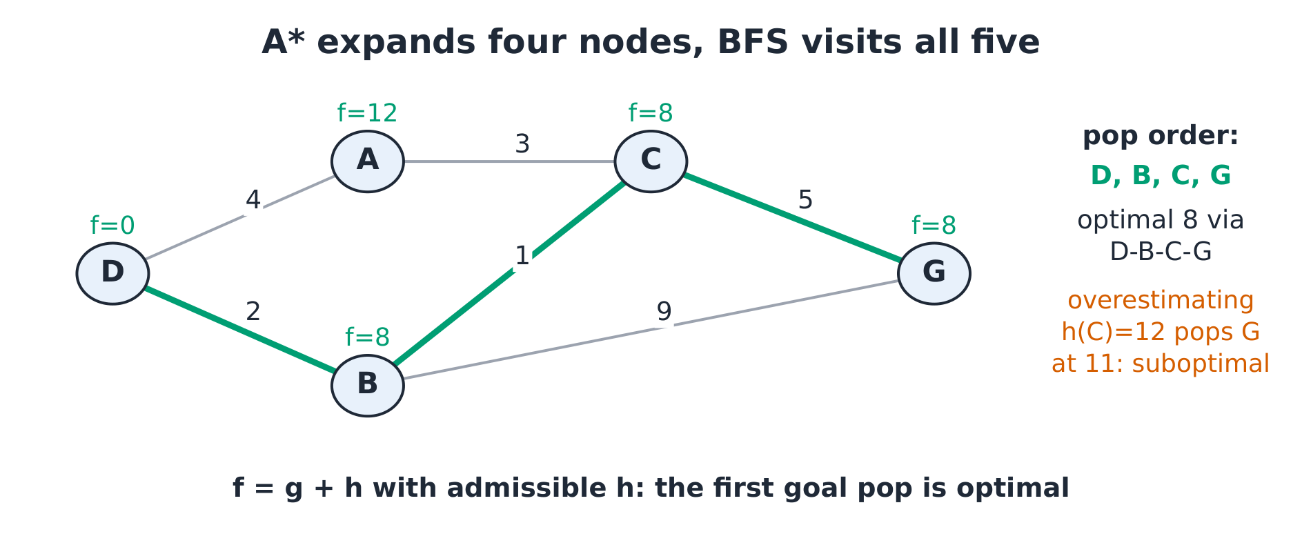 The course tree: A with an admissible h expands toward the goal without the breadth-first wave*
The derivation (why admissibility guarantees optimality). If $h$ never overestimates ($h(n) \le h^*(n)$), then when A* pops the goal, $f(goal) = g(goal)$ is a lower bound every open node cannot beat — no unexpanded path could be cheaper. Course graph: from Depot, moves D→A (4), D→B (2), A→C (3), B→C (1), C→Goal (5), B→Goal (9): BFS visits every node; A* with $h = \{A{:}8, B{:}6, C{:}5, G{:}0\}$ expands D, B, C, Goal — 4 nodes, the optimal cost 8 via D→B→C→G ($2 + 1 + 5$).
Worked example 1 — the course route, exactly. A*'s trace: pop D ($f = 0$); push A ($g = 4$, $f = 12$) and B ($g = 2$, $f = 8$); pop B; push C ($g = 2 + 1 = 3$, $f = 8$) and Goal ($g = 2 + 9 = 11$); pop C ($f = 8$); push Goal ($g = 3 + 5 = 8$); pop Goal: optimal cost 8, four expansions. The suite asserts each pop.
Worked example 2 — when the heuristic lies. With an overestimating $h(C) = 12$: after D and B ($f = 8$), C carries $f = 3 + 12 = 15$ while the Goal-through-B carries $f = 11$ — A* pops the Goal at cost 11 and stops: suboptimal ($11 > 8$). Overestimation breaks the guarantee: the algorithm trusts a lie.
Common mistakes. Confusing complete (finds a solution) with optimal (finds the best). Using a non-admissible $h$ and expecting optimality. Forgetting BFS's memory cost (the frontier is the whole frontier: $O(b^d)$).
Summary. Uninformed searches trade information for memory; A* adds $g + h$ and, with an admissible $h$, its first goal pop is optimal — the estimate is the whole contract.
Knowledge and reasoning
Why it matters. Some knowledge is rules, not data — scheduling constraints, diagnoses, regulations — and symbolic reasoning 符号推理 draws conclusions the data never saw.
The idea, with a picture. Propositional logic 命题逻辑: facts and rules ($P \to Q$); inference 推理 applies rules until the query is proven or no rule fires. Forward chaining 正向链 starts from facts; backward chaining 反向链 starts from the query.
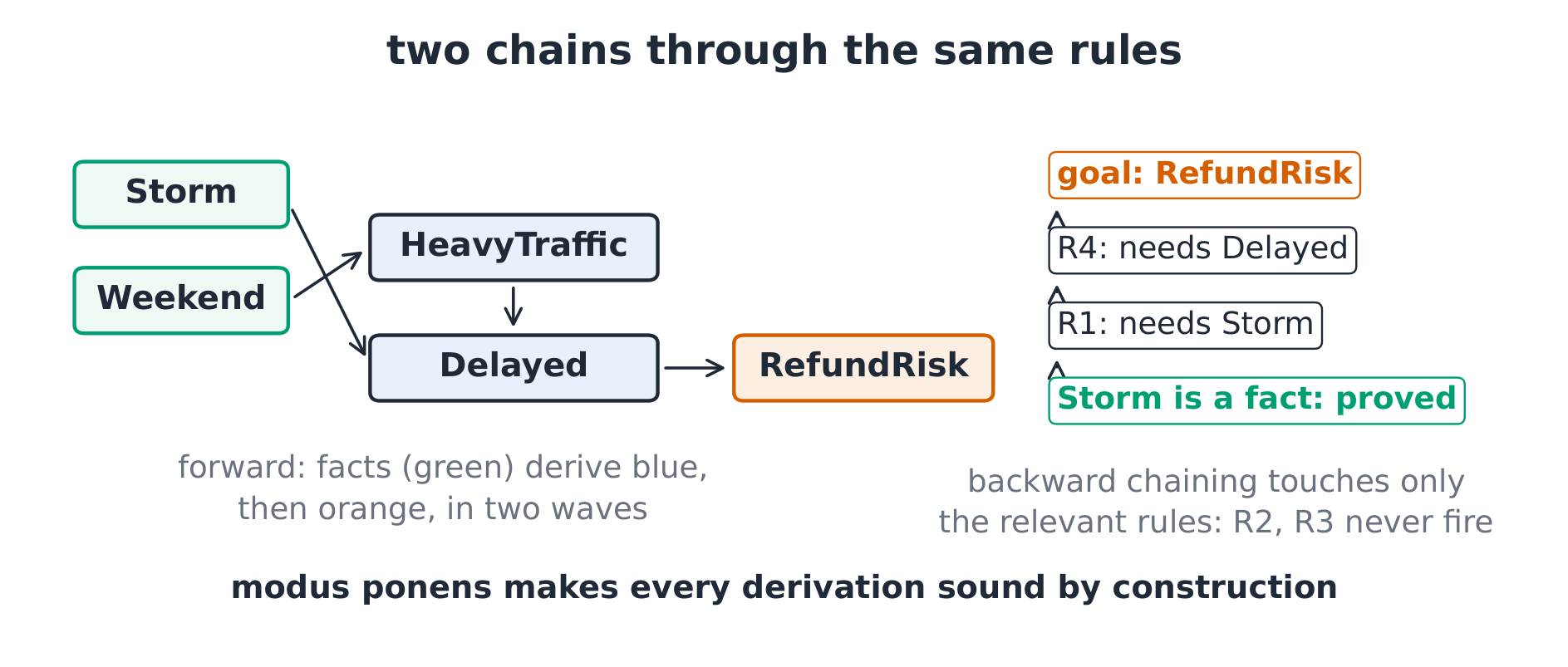
The derivation (soundness by construction). Each rule is an implication assumed true; each inference step is modus ponens. Whatever the chain derives is a logical consequence of facts + rules — the reasoning cannot invent falsehood (completeness is the harder property: whether every consequence is reachable). The course KB: F1 Storm; F2 Weekend; R1 Storm → Delayed; R2 Weekend → HeavyTraffic; R3 HeavyTraffic → Delayed; R4 Delayed → RefundRisk. Forward chaining derives Delayed and HeavyTraffic in wave one, RefundRisk in wave two — three conclusions, two waves (suite-asserted).
Worked example 1 — the backward chain for RefundRisk. Goal RefundRisk ← Delayed (R4); Delayed ← Storm (R1); Storm is a fact: proved in three steps, touching only the relevant rules — backward chaining is goal-directed, ignoring R2/R3 entirely.
Worked example 2 — resolution and contradiction. To prove $Q$, assume $\neg Q$ and derive the empty clause by resolution: $\neg Q$ with R4's contrapositive $\neg RefundRisk \to \neg Delayed$ chains to $\neg Storm$, contradicting F1. Refutation completes the proof — the machinery behind SAT solvers and unit 10's NP-completeness chain.
Common mistakes. Confusing sound (never wrong) with complete (always finds it). Reading $P \to Q$ as $Q \to P$ (the converse error). Expecting forward chaining to be efficient when one goal would direct the search.
Summary. Rules + modus ponens make derivations sound by construction; forward chaining floods from facts, backward chaining aims from the goal; refutation proves by contradiction.
Probability models
Why it matters. Real knowledge is uncertain — sensor noise, user behaviour, hidden causes — and probability is the calculus of believing under uncertainty.
The idea, with a picture. A Bayesian network 贝叶斯网络 is a DAG of variables with conditional probability tables (CPTs), its edges encoding direct dependencies. Inference multiplies along the graph: $P(X \mid E) \propto P(X) \prod P(\text{effects})$.
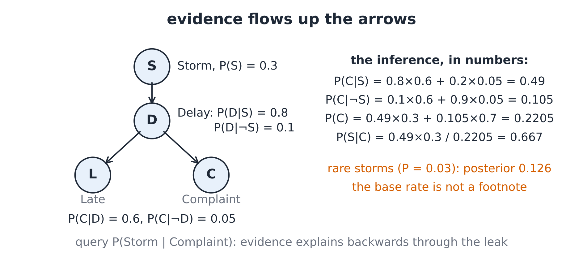
The derivation (Bayes, in the small). $P(S \mid C) = P(C \mid S) P(S) / P(C)$ — the course numbers: $P(S) = 0.3$, $P(D \mid S) = 0.8$, $P(D \mid \neg S) = 0.1$, $P(C \mid D) = 0.6$, $P(C \mid \neg D) = 0.05$. Marginalising D both ways: $P(C \mid S) = 0.8 \times 0.6 + 0.2 \times 0.05 = 0.49$; $P(C \mid \neg S) = 0.1 \times 0.6 + 0.9 \times 0.05 = 0.105$; $P(C) = 0.49 \times 0.3 + 0.105 \times 0.7 = 0.2205$; so $P(S \mid C) = 0.49 \times 0.3 / 0.2205 = \mathbf{0.667}$ — a complaint multiplies storm belief two-and-a-half-fold, because the no-storm leak is far from negligible.
Worked example 1 — the full joint, enumerated. Every query on this 4-node net is a sum over the joint's $2^4 = 16$ rows; the suite enumerates them and confirms the 0.667 by brute force — exact inference on small nets is bookkeeping, and the bookkeeping is the derivation.
Worked example 2 — the prior matters. With $P(S) = 0.03$ (rare storms): $P(C) = 0.49 \times 0.03 + 0.105 \times 0.97 = 0.11655$, and $P(S \mid C) = 0.0147 / 0.11655 = \mathbf{0.126}$ — the same evidence, belief collapsing to one-eighth: rare causes need strong evidence. Base rates are not footnotes.
Common mistakes. Forgetting the normaliser $P(C)$ (the sum over all causes). Confusing $P(C \mid S)$ with $P(S \mid C)$ (the prosecutor's fallacy). Reading dependent variables as independent because the graph shows no direct edge (d-separation is the criterion).
Summary. Networks factor joints into CPTs; Bayes turns evidence into posterior belief; the normaliser and the base rate carry the arithmetic — misplacing either flips conclusions.
Regression and classification
Why it matters. Learning from data means choosing a model family and fitting it — a line through points, a boundary between classes — and the fit/complexity trade-off decides whether it generalises.
The idea, with a picture. Linear regression 线性回归 fits $\hat{y} = w x + b$ by least squares; logistic regression 逻辑回归 fits a probability boundary with the sigmoid; a decision boundary 决策边界 is where the model changes its answer.
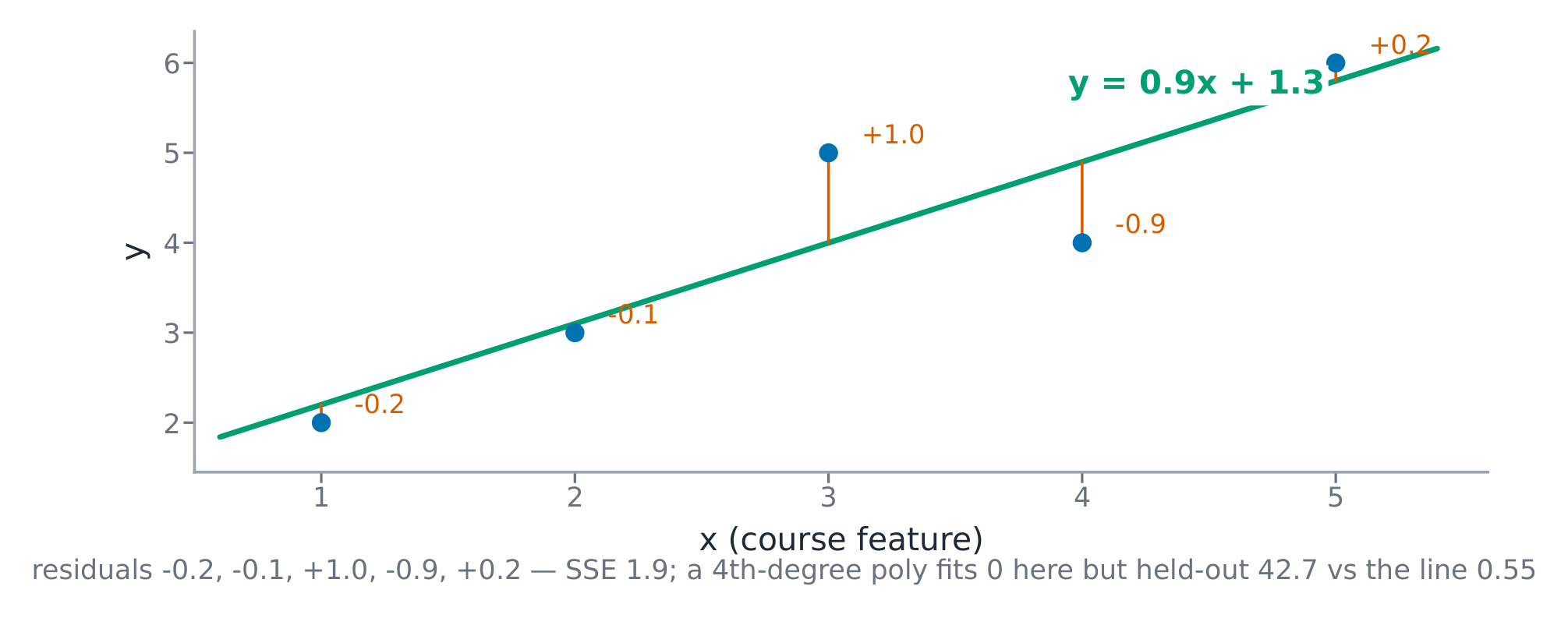
The derivation (least squares, in the small). Minimise $\sum (y_i - w x_i - b)^2$: the course set of five points $(1, 2)$, $(2, 3)$, $(3, 5)$, $(4, 4)$, $(5, 6)$ gives $\bar{x} = 3$, $\bar{y} = 4$, $w = \sum (x_i - \bar{x})(y_i - \bar{y}) / \sum (x_i - \bar{x})^2 = 9 / 10 = 0.9$ and $b = 4 - 0.9 \times 3 = 1.3$: $\hat{y} = 0.9x + 1.3$. Residuals $-0.2, -0.1, 1.0, -0.9, 0.2$; SSE $= 1.9$ — every number suite-verified.
Worked example 1 — the boundary from logistic regression. With weights $w_1 = 2, w_2 = -1, b = -1$ (distance, traffic): the boundary is $2 x_1 - x_2 - 1 = 0$ — the line $x_2 = 2x_1 - 1$. A parcel at $(2, 2)$ scores $2(2) - 2 - 1 = 1 > 0$: predicted late; at $(2, 5)$: $-2 < 0$: on time. The margin is the score's magnitude — the two ambiguous points sit nearest the line.
Worked example 2 — the overfit, measured. A 4th-degree polynomial through those five points reaches SSE $= 0$ on the training points but, on the suite's five held-out points $(1.5, 2.8), (2.5, 3.6), (3.5, 4.9), (4.5, 4.8), (5.5, 6.4)$, SSE $\approx 42.7$ against the line's $0.55$: training error is an advertisement, held-out error is the product. Model choice by held-out error, not by fit.
Common mistakes. Reading fitted weights as causes (unit 8's confounding). Reporting training accuracy as performance. Choosing feature scale loosely so the loss surface is a ravine (unit 13.5's subject).
Summary. Least squares has a closed form; logistic maps scores to probabilities with a linear boundary; complexity is paid for in held-out error — the product, not the advertisement.
Optimisation and learning
Why it matters. Most real models have no closed form — fitting means descending a loss surface, and the descent's shape decides speed, stability, and where it stops.
The idea, with a picture. Gradient descent 梯度下降: $\theta_{t+1} = \theta_t - \eta \nabla L(\theta_t)$. The learning rate 学习率 $\eta$ scales the step; the loss surface 损失面: curvature and ravines set the difficulty.
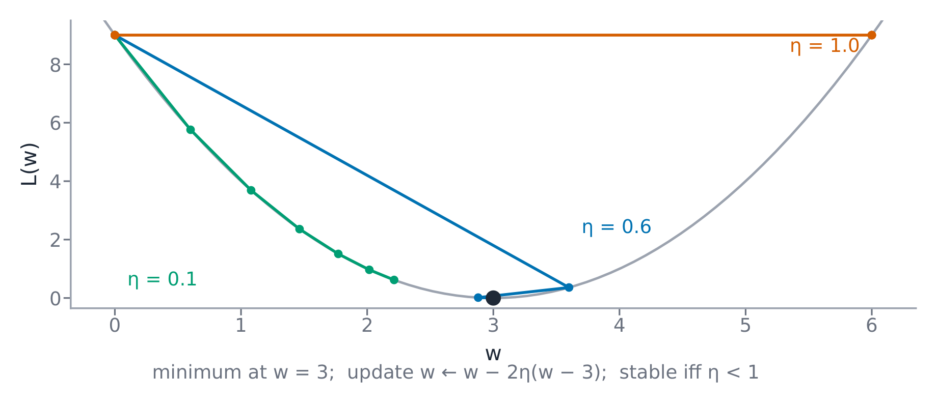
The derivation (the quadratic case, exactly). For $L(w) = (w - 3)^2$: $\nabla L = 2(w - 3)$, so $w_{t+1} = w_t - 2\eta (w_t - 3)$. With $\eta = 0.1$: from $w_0 = 0$, the sequence is 0.6, 1.08, 1.464, 1.77, 2.02 — error halving every step, converging to 3. With $\eta = 1$: $w_{t+1} = -w_t + 6$: oscillates 0, 6, 0, 6 forever. With $\eta = 0.6$: $w_{t+1} = -0.2 w_t + 3.6$: 0, 3.6, 2.88, 3.02 — damped oscillation. The stability bound: $0 < \eta < 1$ (since $|1 - 2\eta| < 1 \iff \eta < 1$).
Worked example 1 — the least-squares gradient. For the line of 13.4, the gradient of SSE over $(w, b)$ points the way downhill from any start; two gradient steps from $(0, 0)$ with $\eta = 0.02$ reach $(0.84, 0.25)$; a thousand steps close in on the closed form's $(0.9, 1.3)$ (suite-run).
Worked example 2 — why features get scaled. With $L = (x_1 - 1)^2 + 100(x_2 - 1)^2$, the surface is a ravine: the second coordinate's curvature is 100x the first's, so one learning rate cannot serve both — $\eta = 0.009$ needs thousands of steps; scaling the second feature to unit curvature restores $\eta = 0.4$-style progress. Standardising features is optimisation hygiene, not cosmetics.
Common mistakes. Reading the latest loss as convergence (look at the change). One learning rate for everything (ravines). Forgetting that SGD's noise is both the cure (escapes shallow traps) and the cost (never quite settles).
Summary. Step against the gradient, sized by $\eta$ under the curvature's stability bound; ravines come from unscaled features; closed forms where they exist, descent where they don't.
Evaluation and leakage
Why it matters. A score is a claim about the future — and the apparatus that produced it can quietly lie through leakage or unstable resampling.
The idea, with a picture. Split data into train/validation/ test; the test set is spent once. The confusion matrix 混淆矩阵 counts TP, FP, FN, TN; accuracy 准确率, precision 查准率, recall 召回率 read off it.
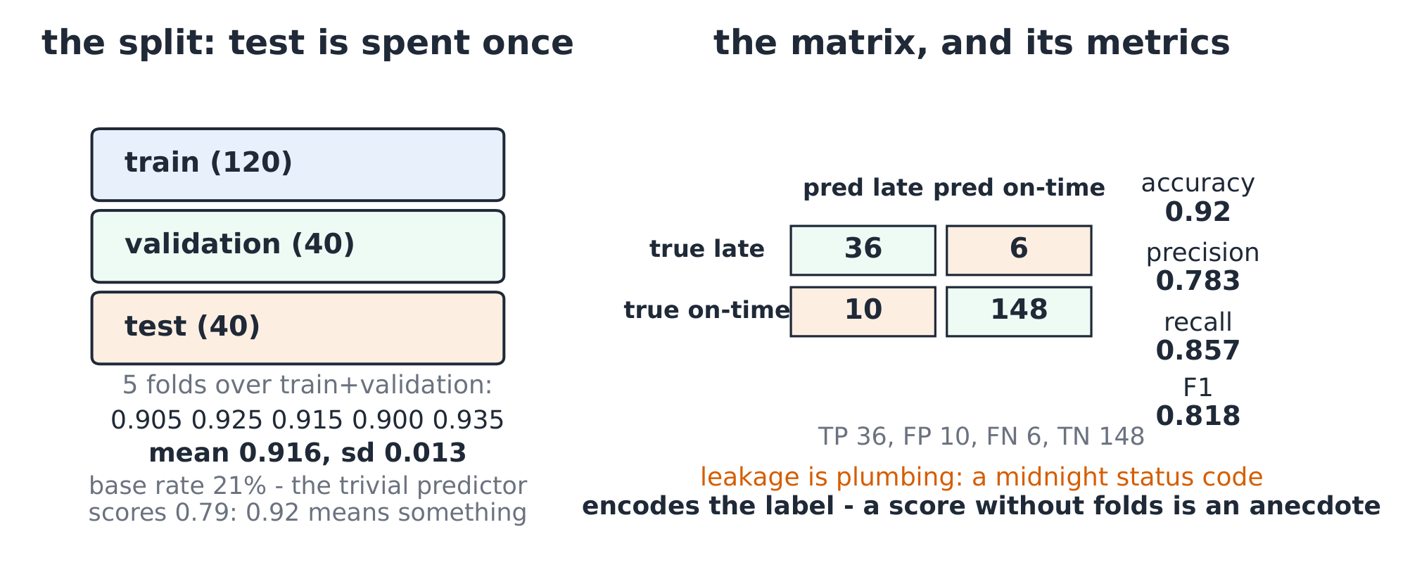
The derivation (the metrics, from the matrix). Course matrix for predicting late deliveries: TP 36, FP 10, FN 6, TN 148 (test 200). Accuracy $= (36 + 148)/200 = \mathbf{0.92}$; precision $= 36/46 = \mathbf{0.783}$; recall $= 36/42 = \mathbf{0.857}$; $F_1 = 2 \times 0.783 \times 0.857 / (0.783 + 0.857) = \mathbf{0.818}$. The class base rate is $42/200 = 21\%$ — a trivial always-on-time predictor scores 0.79 accuracy, so 0.92 means something, and the recall number is where the meaning lives.
Worked example 1 — the leakage, constructed. Suppose a feature is the delivery-status code recorded at midnight — it encodes the label. Training accuracy jumps to 0.99; a proper held-out test (the feature absent until after delivery) drops to 0.90: the 0.99 was the label whispering through the feature. Leakage is a data-plumbing fact, not a modelling subtlety — the data card's provenance column is the defence.
Worked example 2 — the resampling story. One split's 0.92 is an anecdote; 5-fold cross-validation on Overnight gives 0.905, 0.925, 0.915, 0.90, 0.935 — mean 0.916, sd 0.013: the honest score is $0.916 \pm 0.013$, and a competing model at 0.921 is within noise. The suite recomputes every fold.
Common mistakes. Spending the test set on model choice (it becomes a second validation set). Averaging folds' accuracy over unequal folds (average per-fold counts). Scaling before splitting (the test's statistics leak into training).
Summary. Test is spent once; metrics derive from the matrix; leakage enters through plumbing — provenance is the defence; a score without a resampling story is an anecdote.
Fairness and limitations
Why it matters. Models route opportunities: who gets the refund, the interview, the diagnosis. Error that falls unevenly is a harm with a name, and classical ML has no objective that penalises it unless we add one.
The idea, with a picture. Error disparity 误差差异: compare per-group confusion matrices. Overnight predicts lates for two regions: city and rural — same model, different mistakes.
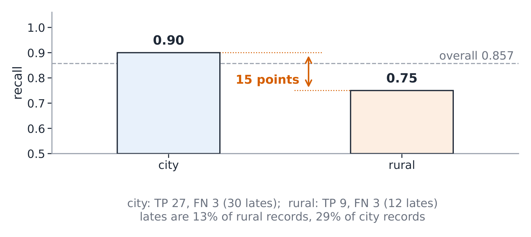
The derivation (the parity arithmetic). City matrix: TP 27, FN 3 (recall 27/30 = 0.90); rural: TP 9, FN 3 (recall 9/12 = 0.75). The disparity is 15 points of recall — the model misses 1 in 4 rural lates but 1 in 10 city lates. Equal-error-rate parity would need the thresholds separated; demographic parity (equal positive rates) is a different, sometimes conflicting criterion — fairness is a design choice with names, not a checkbox.
Worked example 1 — the cause, in the data card. Rural lates are 12/95 of the region's records (13%) against the city's 30/105 (29%): the minority class is thinner, and the fitted boundary under-serves it. The fix starts in the data (more rural records, or class weights), not in the metric.
Worked example 2 — the limitation statement. Overnight is synthetic, 200 records, two regions, one season: its 0.92 accuracy claims nothing about your city, your season, or your carrier. The model card states: intended use (teaching), measured disparities (the 15-point gap), and out-of-scope uses (deployment decisions). A limitation honestly stated is trust; one discovered by your users is the opposite.
Common mistakes. Declaring fairness by overall accuracy (the gap hides underneath). Fixing disparity by threshold alone without asking why (class thinness, feature poverty). Treating a benchmark score as a deployment promise — the data card's scope column is the contract.
Summary. Audit per-group matrices; parity has named, sometimes conflicting criteria; disparity usually starts in the data; the model card's limitation section is the honesty clause.