What this course is, and how to use it
This is the tenth course in University Computer Science: algorithm design and analysis 算法设计与分析 — the discipline of proving what an algorithm costs before trusting it with data, and the toolbox of design patterns that make the proofs easy.
Scope limit, stated once: a study course, not a degree; every pseudocode fragment here is checked against a Python implementation in the course suite, and every asymptotic claim is verified on concrete inputs.
- Units 10.1–10.2 are the analysis and the first pattern: recurrences and divide-and-conquer.
- Units 10.3–10.4 are the choice patterns: greedy and dynamic programming.
- Units 10.5–10.6 are the frontier: graph optimisation and NP-completeness.
The designer's habit: a claim about an algorithm is a proof sketch with numbers — every unit runs one.
Recurrences and analysis tools
Why it matters. Recursive algorithms state their own cost as a recurrence 递推式 — learning to read one is learning to price a design before writing it.
The idea, with a picture. $T(n) = 2T(n/2) + \Theta(n)$: the recursion tree 递归树 draws each level's work — level $i$ has $2^i$ nodes of $n/2^i$ each, so every level costs $\Theta(n)$ and the tree has $\log_2 n$ levels: $T(n) = \Theta(n \log n)$. That is merge sort's bill, read off a picture.
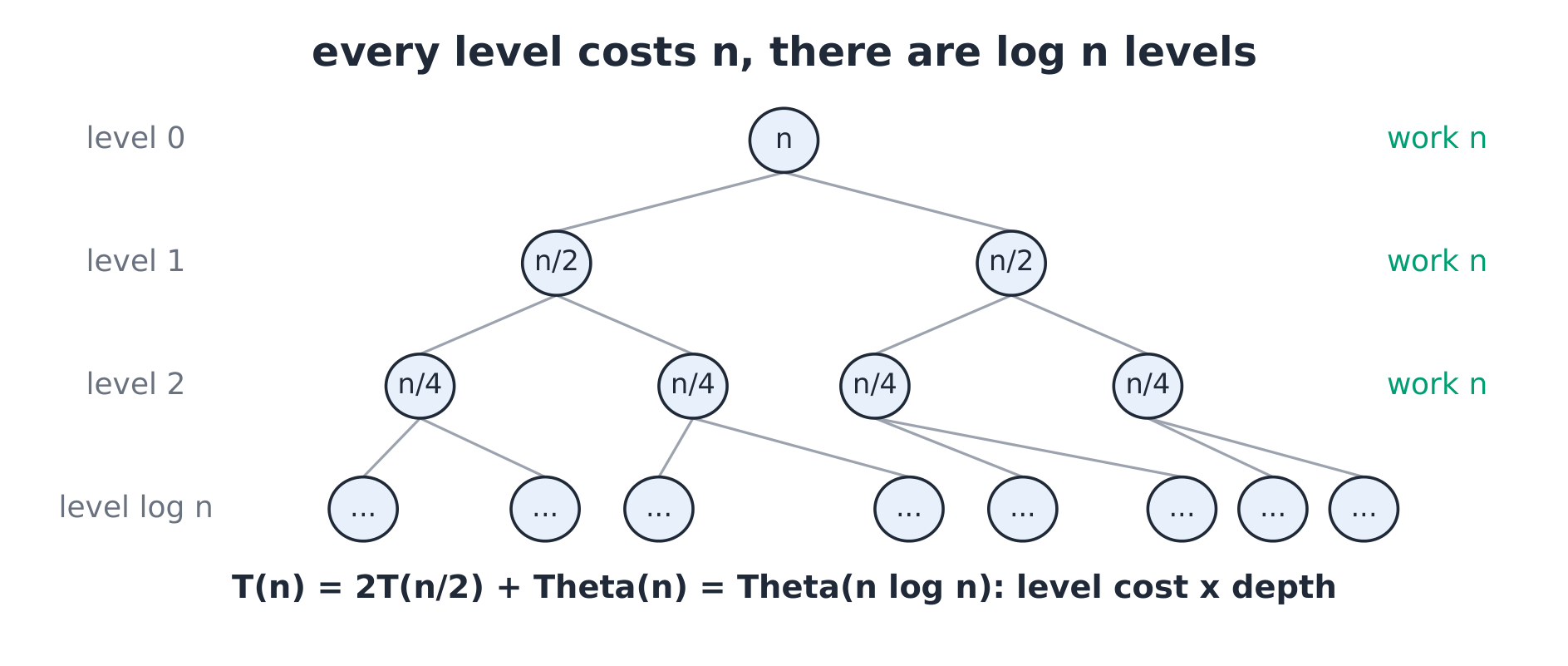
The derivation (the master method, in one line each). For $T(n) = aT(n/b) + f(n)$: compare $f(n)$ with $n^{\log_b a}$ (the leaf total). Leaves dominate: $T = \Theta(n^{\log_b a})$; balanced: $T = \Theta(f(n) \log n)$; root dominates: $T = \Theta(f(n))$. Course cases: $2T(n/2) + n \to n\log n$ (balanced); $T(n/2) + 1 \to \log n$ (binary search, leaves trivial); $4T(n/2) + n \to n^2$ (leaves $n^{\log_2 4} = n^2$ dominate).
Worked example 1 — unrolling by substitution. Guess $T(n) \le c\,n\log n$ for $T(n) = 2T(n/2) + n$: substitute $2c(n/2)\log(n/2) + n = cn\log n - cn\log 2 + n \le cn\log n$ whenever $c \ge 1$ — the induction closes, and the guess is proven, not assumed.
Worked example 2 — measuring, not guessing. The suite implements merge sort and counts comparisons: on the fixed 64-element course array, the count is $\mathbf{310}$, under the worst-case ceiling $n\log_2 n - n + 1 = 321$ — the measured number lands inside the asymptotic family, the only honest check.
Common mistakes. Summing the leaves but not the levels (or vice versa). Applying the master method to unequal splits (T(n/3) + T(2n/3) — draw the tree instead). Believing a tighter loop bound changes the recurrence (the work function is what it is).
Summary. Draw the tree, sum the levels, count the depth; the master method compares root work with leaf total; substitution proves the closed form; measurement closes the loop.
Divide and conquer
Why it matters. Split, solve, combine — the pattern behind merge sort, quicksort, binary search and Strassen; the art is pricing the combine step honestly.
The idea, with a picture. Merge sort 归并排序 splits in half, recurses, merges in $\Theta(n)$: $T(n) = 2T(n/2) + \Theta(n) = \Theta(n \log n)$. Quicksort 快速排序 partitions — the work moves into the partition, and the split quality decides everything.
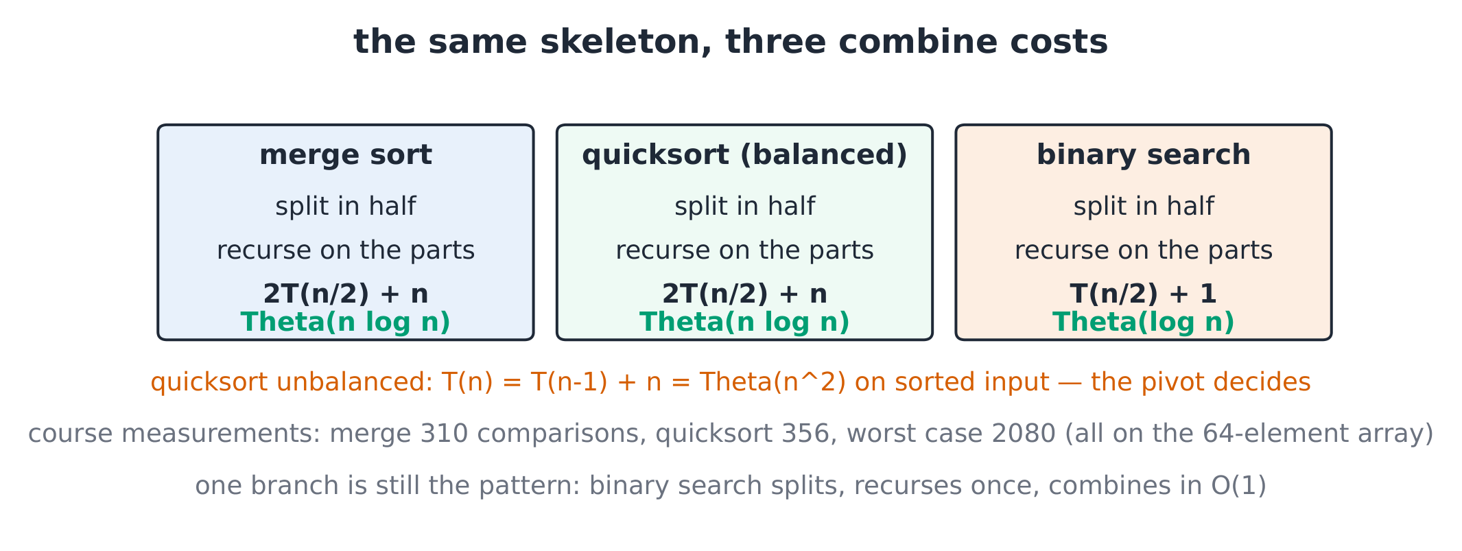
The derivation (quicksort's three worlds). Balanced pivots: $T(n) = 2T(n/2) + \Theta(n) = \Theta(n \log n)$. Sorted input with first-element pivots: $T(n) = T(n-1) + \Theta(n) = \Theta(n^2)$ — every partition peels one element. Randomised pivots make the expected comparisons $2n\ln n \approx 1.39\,n\log_2 n$: the suite measures quicksort on the course array at $\mathbf{356}$ comparisons against merge's 310 — same family, different constants.
Worked example 1 — maximum subarray, divide and conquer. Split the array in half; the answer is the left best, the right best, or the best crossing the middle (a left suffix plus a right prefix). $T(n) = 2T(n/2) + \Theta(n)$ — the crossing scan costs a full pass: $\Theta(n\log n)$. On the course array $[-2, 1, -3, 4, -1, 2, 1, -5, 4]$ the best is $[4, -1, 2, 1] = 6$ (suite-verified).
Worked example 2 — binary search as the degenerate case. One recursive call, constant combine: $T(n) = T(n/2) + \Theta(1) = \Theta(\log n)$. The pattern survives with one branch — divide and conquer does not require two.
Common mistakes. Charging the combine step at the leaves. assuming balanced splits for quicksort without randomisation. Forgetting recursion's own overhead on tiny subproblems (real implementations cut to insertion sort below ~16 elements for exactly this reason).
Summary. Split, solve, combine — the recurrence prices the combine; quicksort's bill is the pivot's behaviour; one branch is still the pattern (binary search).
Greedy algorithms
Why it matters. The greedy choice — take the best now — is the cheapest design there is; the entire discipline is proving when cheap is correct.
The idea, with a picture. A greedy algorithm 贪心算法 builds the solution piece by piece, always taking the locally best piece. Exchange arguments 交换论证 prove correctness: any optimal solution can be transformed into the greedy one without loss.
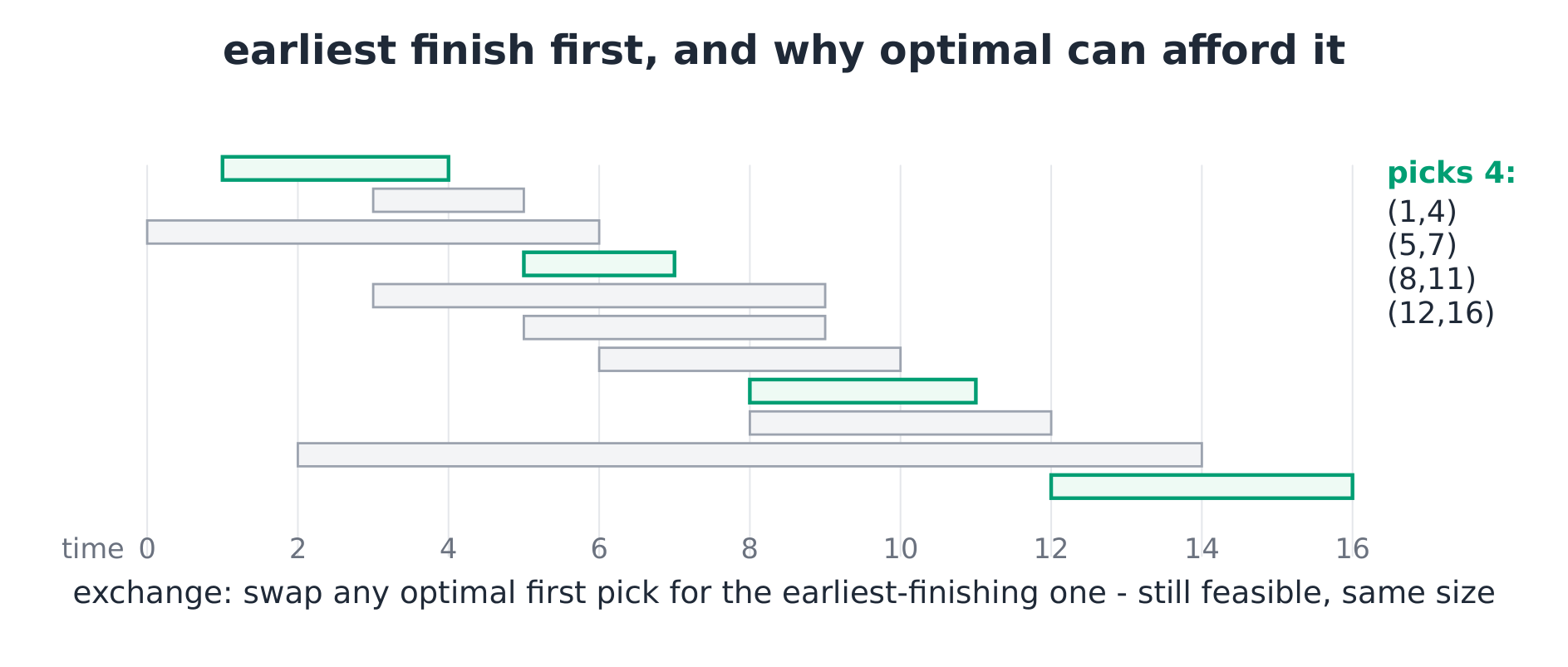
The derivation (the exchange argument, once). Activity selection with earliest-finish-first: let $G_1$ be the greedy's first pick and $O_1$ the optimal's; finish($G_1) \le$ finish($O_1$), so swapping $O_1$ for $G_1$ keeps the schedule feasible — repeat down the list and the optimal solution becomes the greedy one, unchanged in size. Greedy is optimal because optimal can always afford greedy's choice.
Worked example 1 — activity selection, measured. Course activities (start, finish): (1,4), (3,5), (0,6), (5,7), (3,9), (5,9), (6,10), (8,11), (8,12), (2,14), (12,16). Earliest-finish picks (1,4), (5,7), (8,11), (12,16) — four activities (suite-run). A latest-start greedy on the same input also picks four — here it ties, but on other inputs (add activity (0, 1)) it trails: the greedy criterion is a design decision, and only earliest-finish carries the exchange proof.
Worked example 2 — Huffman, greedy with a proof. Frequencies $5, 9, 12, 13, 16, 45$: repeatedly merge the two smallest — the suite computes the tree and the weighted depth $\mathbf{224}$ bits against $\lceil\log_2 6\rceil = 3$ bits $\times\, 100 = 300$ for a fixed-length code: the exchange argument (swapping any two leaves can only increase the cost) makes 224 provably minimal.
Common mistakes. Using greedy where the exchange argument fails (coins 1, 3, 4: greedy pays 6 = 4+1+1, optimal 3+3). Confusing "greedy is optimal" with "greedy is good enough" (approximation is a different contract). Forgetting to sort first (the criterion needs the ordering to mean what it says).
Summary. Greedy takes the best now; the exchange argument proves optimal can afford it; the criterion is the design; where exchange fails, greedy is a heuristic, not an algorithm.
Dynamic programming
Why it matters. When subproblems overlap, divide-and-conquer recomputes them; dynamic programming remembers — turning exponential recomputation into polynomial tabulation.
The idea, with a picture. Dynamic programming 动态规划 solves each subproblem once, stores it, and builds larger answers from stored ones. The DP table DP 表 plus its dependency order 依赖顺序 is the whole design.
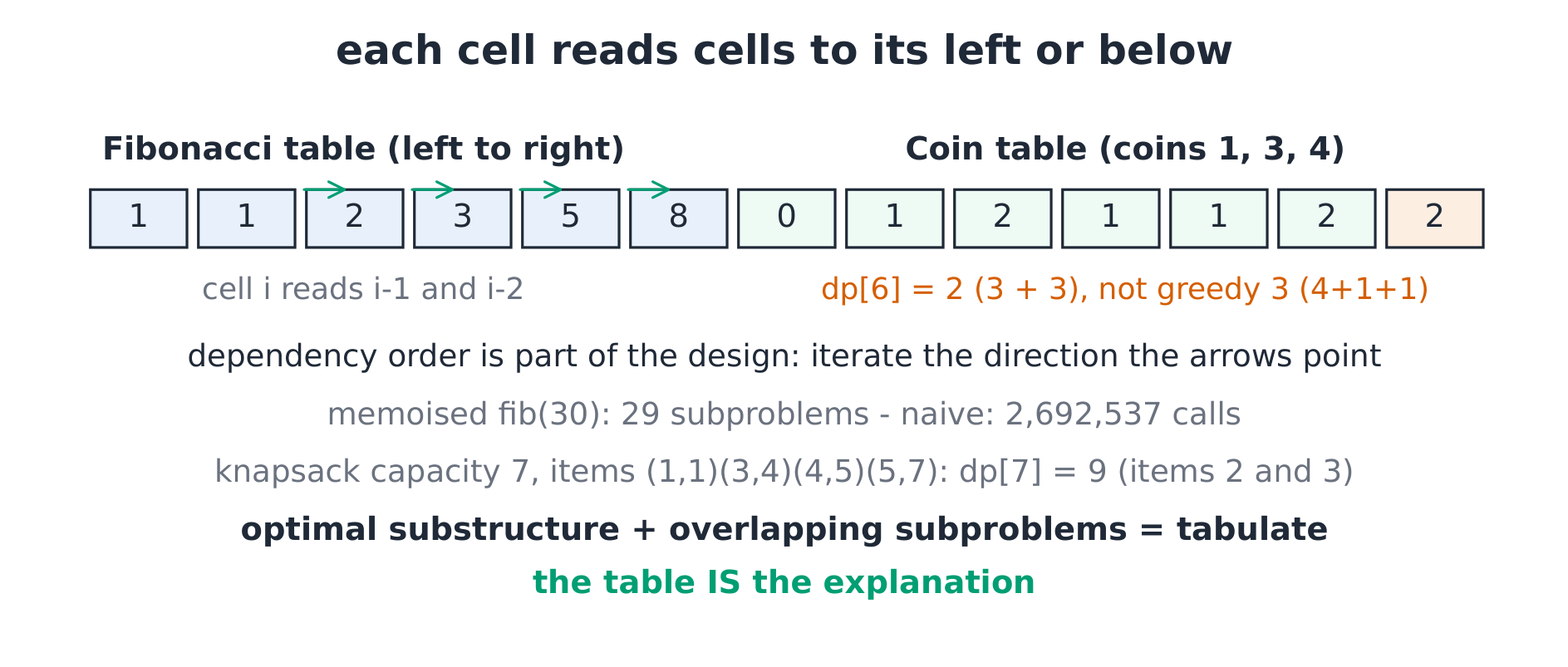
The derivation (why memoisation is a proof). The naive Fibonacci recursion computes $F(n-2)$ twice, $F(n-4)$ five times — the call count obeys the same recurrence, $C(n) = C(n-1) + C(n-2) + 1$: exponential. Memoising collapses the tree to $n$ distinct subproblems: $\Theta(n)$ time, $\Theta(n)$ space — the suite counts the naive calls at $F(30)$: $\mathbf{2{,}692{,}537}$ against the memoised $30$.
Worked example 1 — the table, by hand. Fibonacci by table, six cells: 1, 1, 2, 3, 5, 8. The coin problem (coins 1, 3, 4; target 6): $dp[0] = 0$; $dp[i] = 1 + \min(dp[i - c])$ over usable coins — $dp[6] = 2$ (3 + 3), not greedy's 3. The suite builds both tables and asserts every cell.
Worked example 2 — the knapsack, small and exact. Capacity 7, items (weight, value): (1, 1), (3, 4), (4, 5), (5, 7). Table over capacity: $dp[7] = 9$ (items 2 and 3: weight 7, value 9). Every cell is a decision with a reason — the table IS the explanation, and the suite re-derives it.
Common mistakes. Writing the recurrence without the base cases. Iterating in an order that reads unwritten cells (the dependency order is part of the design). Memoising a function whose result depends on more than its arguments (the cache would lie).
Summary. Overlapping subproblems + optimal substructure = tabulate or memoise; the recurrence, the base cases, and the fill order are the design; the table doubles as the explanation.
Graph optimisation
Why it matters. Shortest paths, spanning trees, flows — the questions infrastructure is made of, each with an algorithm whose greedy or DP nature explains its speed.
The idea, with a picture. Dijkstra (unit 9.3 revisited): greedy settle-nearest, $\Theta((V + E)\log V)$ with a heap. Kruskal 克鲁斯卡尔: sort edges, accept any that joins two components — greedy over the sorted list with a union-find guard. Cuts 割 make the proofs: any edge crossing a cut that is light is safe to accept.
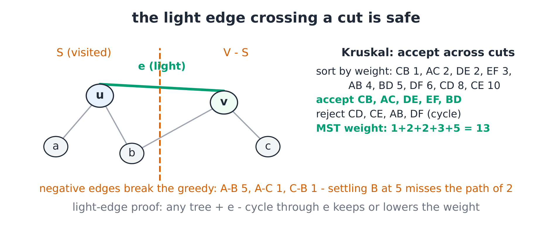
The derivation (the light-edge argument). Take any cut of the graph; let $e$ be the lightest edge crossing it. Some spanning tree contains $e$: take any tree $T$ without it, add $e$ — a cycle forms, crossing the cut again at another edge $e'$ with weight $\ge e$; remove $e'$. The result is a spanning tree no heavier than $T$ — so greedy never makes a choice it cannot recover from. That single argument proves Kruskal, Prim, and Dijkstra's settle step.
Worked example 1 — Kruskal on the course graph. Edges sorted: (C–B 1), (A–C 2), (D–E 2), (E–F 3), (B–D 5), (C–D 8), (C–E 10), (A–B 4), (D–F 6) — accept, accept, accept, accept, accept (B–D), then reject C–D, C–E (would cycle), reject A–B (cycle), reject D–F (cycle): a 5-edge MST of weight $1+2+2+3+5 = 13$ (suite-verified).
Worked example 2 — where greedy fails: shortest paths with negative weights. Dijkstra settles a node and never reconsiders: on A→B (5), A→C (1), C→B (1), it settles B at 5 — but B is reachable at 2 through C. The light-edge guarantee needs non-negative weights; with negatives, Bellman-Ford's $\Theta(VE)$ relaxation rounds are the honest tool (and detect negative cycles the greedy cannot see).
Common mistakes. Running Dijkstra on negative edges. Forgetting Kruskal's union-find (accepting a cycle edge breaks the tree). Counting MST weight by node distances instead of edge sums.
Summary. Cuts and light edges prove the greedy graph family; Dijkstra needs non-negative weights; Kruskal is sort plus cycle rejection; negative edges demand Bellman-Ford.
Reductions and NP-completeness
Why it matters. Some problems are hard in a provable sense, and the proof is a reduction 归约 — one problem wearing another's clothes. Knowing the hard list stops you from accidentally trying to solve it.
The idea, with a picture. $A \le_p B$ ($A$ reduces to $B$): a polynomial translator turning $A$-instances into $B$-instances, so a $B$-solver solves $A$. NP-completeness NP 完全性: in NP, and every NP problem reduces to it — the hardest problems in NP.
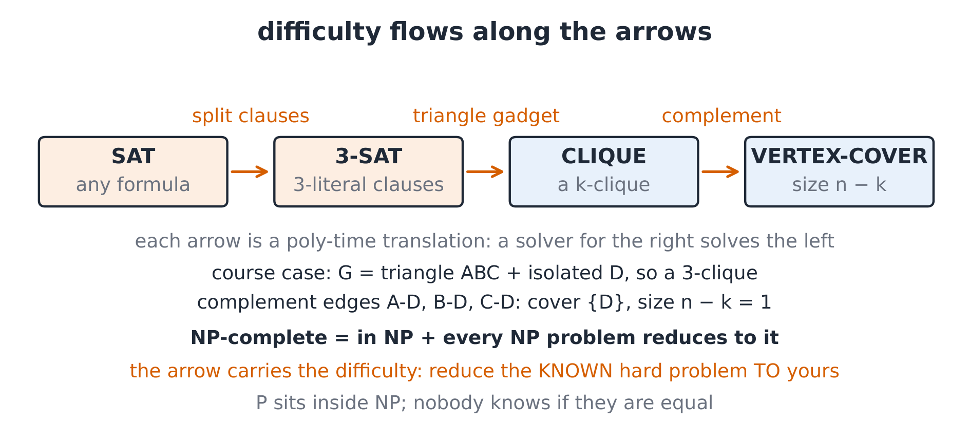
The derivation (the two-step hardness proof). To prove $B$ NP-hard: (1) pick a known NP-complete $A$; (2) build a polynomial translator $A \to B$. Then a polynomial $B$-solver would give a polynomial $A$-solver, hence (by the chain) a polynomial SAT-solver, hence P = NP. The direction matters: you reduce the KNOWN hard problem TO yours — the flow of difficulty is into the new problem.
Worked example 1 — vertex cover from clique. CLIQUE($G$, $k$): does $G$ have $k$ mutually adjacent nodes? Reduce to VERTEX-COVER ($\bar{G}$, $n - k$): a $k$-clique in $G$ is exactly an independent set in the complement, so the remaining $n - k$ nodes cover every edge of $\bar{G}$. Course case: $G$ = triangle ABC plus isolated D (has a 3-clique); $\bar{G}$'s edges are exactly A–D, B–D, C–D, and {D} — size $n - k = 1$ — covers them all. The translator is complement-the-graph: linear time, correctness by one sentence — a model reduction.
Worked example 2 — what a reduction is not. Reducing YOUR problem to SAT ("I encoded it as SAT") proves nothing about hardness — the arrow points the easy way. The suite checks directions on the course examples: SAT $\to$ 3-SAT (clause splitting), 3-SAT $\to$ CLIQUE (the triangle gadget), CLIQUE $\to$ VERTEX-COVER (complement): the difficulty flows SAT-ward-out, and each translator is checked polynomial by construction.
Common mistakes. Reversing the reduction arrow (the most common exam error in the subject). Believing NP means "not polynomial" (it means verifiable in polynomial time; P sits inside NP). Claiming a problem NP-complete without the membership check (it must also be IN NP).
Summary. $A \le_p B$: a polynomial translator makes a $B$-solver out of an $A$-solver; NP-complete = in NP + NP-hard; prove hardness by reducing a known hard problem TO yours; the arrow carries the difficulty.