このプリントは、トピック 1:純数学(Further Pure Mathematics) 1 を扱っています。新しい代数、行列、極座標、より高度なベクトル、帰納法による証明が追加されます。
高等純数学1
Aレベル追加数学 · トピック 1
 14:28
14:28
高等純数学1
ここでは三次方程式を示す。3つの根で軸と交差している。それらの根を正確に求めるのは難しい——あるいは手作業では不可能でさえある。しかしここに美しい…
英語ナレーション・英語+中文字幕 burning-in
1.1
多項式方程式の根
シラバス
| 受験者は以下のことをできること: | メモと例 |
|---|---|
| • 多項式方程式の解と係数の間の関係 recallingして使用すること | 例:解の対称関数を評価したり、方程式の未知係数を含む問題を解くために使用します;次数2, 3, 4の方程式に限定されます。 |
| • 置換を使用して、元の方程式の解と単純な関係にある解を持つ方程式を得ること | 最も簡単な場合、例えば新しい解が逆数または平方、あるいは古い解の単純な線形関数である場合などについては、置換は与えられない。 |
出典: Cambridge International シラバス
多項式方程式において、根は係数と関連しています。$ax^2 + bx + c = 0$ の根が $\alpha, \beta$ の場合:
$$\alpha + \beta = -\frac{b}{a}, \qquad \alpha\beta = \frac{c}{a}.$$
立方方程式 $ax^3 + bx^2 + cx + d = 0$ の根が $\alpha, \beta, \gamma$ の場合:
$$\sum\alpha = -\frac{b}{a}, \qquad \sum\alpha\beta = \frac{c}{a}, \qquad \alpha\beta\gamma = -\frac{d}{a}.$$
$\sum\alpha$ や $\sum\alpha\beta$ のような和は、根の対称関数です(根を入れ替えても値は変わりません)。根が単純に変化した方程式を求めるには、置換を使用します(例:$w = \alpha + 1$ を代入する)。
** worked example(例題).** 方程式 $x^2 - 5x + 6 = 0$ の根は $\alpha, \beta$ です。根が $\alpha + 1, \beta + 1$ となる方程式を求めよ。
ここで $\alpha + \beta = 5$ および $\alpha\beta = 6$ です。新しい和は $(\alpha + 1) + (\beta + 1) = 7$ 、新しい積は $(\alpha + 1)(\beta + 1) = \alpha\beta + \alpha + \beta + 1 = 6 + 5 + 1 = 12$ です。したがって、新しい方程式は以下となります
$$x^2 - 7x + 12 = 0.$$
探索
多項式の解
y = ax³ + bx² + cx + d
解とは曲線がx軸と交わる点であり、それらの和と積は係数と関連している。
1.2
有理関数とグラフ

シラバス
| 受験者は以下のことをできること: | メモと例 |
|---|---|
| • 分子と分母の次数が最大2次の場合の simple 有理関数のグラフを描くこと、斜め漸近線の決定を含む | 関数の値の範囲の決定を含む(例:判別式の使用)。曲線の詳細なプロットは必要ないが、スケッチでは一般的に極点、漸近線、および軸との交点などの重要な特徴を示すことが期待される。 |
| • $y = f(x)$、$y^2 = f(x)$、$y = \frac{1}{f(x)}$、$y = |f(x)|$、$y = f(|x|)$ のグラフ間の関係を理解して使用すること | 方程式や不等式の解法の過程で此类のスケッチグラフを使用する場合を含む。 |
出典: Cambridge International シラバス
有理関数とは、2つの多項式の分数です。分子の次数が分母の次数よりちょうど1高い場合、グラフには斜線渐近線(曲線に近づく傾いた直線)が存在し、割り算によって求めることができます。また、$y = f(x)$ のグラフを、$y^2 = f(x)$ 、$y = \dfrac{1}{f(x)}$ 、$y = |f(x)|$ 、$y = f(|x|)$ のグラフと関連づけることも必要です。判別式を用いて関数が取りうる値の範囲を求め、変曲点の位置を特定してください。
** worked example(例題).** $y = \dfrac{x^2 + x + 1}{x + 1}$ の斜線渐近線を求めよ。
分数を割り算する: $\dfrac{x^2 + x + 1}{x + 1} = x + \dfrac{1}{x + 1}$。$x \to \pm\infty$ 余りが $\dfrac{1}{x+1} \to 0$ であるため、曲線は直線 $y = x$ に漸近する — これが斜め漸近線である。
探索
有理関数
y = a/(x − b) + c
有理関数は、曲線が近づき却始终触れない漸近線を持つ。
語彙
練習する
| English | 日本語 |
|---|---|
| Further Pure Mathematics/ˈfɜːðə pjʊə ˌmæθɪˈmætɪks/ | 純数学(Further Pure Mathematics) |
| roots/ruːts/ | 根 |
| coefficients/ˌkəʊɪˈfɪʃənts/ | 係数 |
| substitution/ˌsʌbstɪˈtjuːʃn/ | 置換反応 |
| rational function/ˈræʃənl ˈfʌŋkʃn/ | 有理関数 |
| oblique asymptote/əˈbliːk ˈæsɪmptəʊt/ | 斜め漸近線 |
| method of differences/ˈmeθəd ɒv ˈdɪfrənsɪz/ | 差分法 |
| convergent/kənˈvɜːdʒənt/ | 収束 |
| sum to infinity/sʌm tʊ ɪnˈfɪnɪti/ | 無限級数の和 |
1.3
級数の和
シラバス
| 受験者は以下のことをできること: | メモと例 |
|---|---|
| • $\sum r$、$\sum r^2$、$\sum r^3$ に対する標準結果を使用して関連する和を見つけること | |
| • 相殺法を使用して有限級数の和を得ること | 一般項を適切な形式で表するために部分分数分解を使用することが必要になることがある。 |
| $n$項までの和を直接考察することで、級数が収束するかどうかを認識し、その場合の無限和を求める |
出典: Cambridge International シラバス
標準的な結果を学ぶ:
$$\sum_{r=1}^{n} r = \tfrac12 n(n+1), \qquad \sum_{r=1}^{n} r^2 = \tfrac16 n(n+1)(2n+1), \qquad \sum_{r=1}^{n} r^3 = \tfrac14 n^2(n+1)^2.$$
差分法は中間項を打ち消し合うことで級数の和を求める方法である:部分分数で各項を $f(r) - f(r+1)$ と書けば、ほぼすべてが打ち消し合う。第$n$項までの和から、その級数が収束するかどうか判断でき、収束すれば無限大の和も求められる。
** worked example.** $\displaystyle\sum_{r=1}^{n} (2r + 1)$ を求める。
$$\sum_{r=1}^{n}(2r + 1) = 2\sum_{r=1}^{n} r + \sum_{r=1}^{n} 1 = 2\cdot\tfrac12 n(n+1) + n = n(n+1) + n = n(n+2).$$
探索
数列とその和
項と累積和をステップバイステップで見る——級数およびその n 項までの和の概念である。
1.4
行列

シラバス
| Candidates should be able to: | Notes and examples |
|---|---|
| carry out operations of matrix addition, subtraction and multiplication, and recognise the terms zero matrix and identity (or unit) matrix | Including non-square matrices. Matrices will have at most 3 rows and columns. |
| recall the meaning of the terms singular and non-singular as applied to square matrices and, for $2 \times 2$ and $3 \times 3$ matrices, evaluate determinants and find inverses of non-singular matrices | The notations $\det \mathbf{M}$ for the determinant of a matrix $\mathbf{M}$, and $\mathbf{I}$ for the identity matrix, will be used. |
| understand and use the result, for non-singular matrices, $(\mathbf{AB})^{-1} = \mathbf{B}^{-1}\mathbf{A}^{-1}$ | Extension to the product of more than two matrices may be required. |
| understand the use of $2 \times 2$ matrices to represent certain geometric transformations in the $x$-$y$ plane, in particular: – understand the relationship between the transformations represented by $\mathbf{A}$ and $\mathbf{A}^{-1}$ – recognise that the matrix product $\mathbf{AB}$ represents the transformation that results from the transformation represented by $\mathbf{B}$ followed by the transformation represented by $\mathbf{A}$ – recall how the area scale factor of a transformation is related to the determinant of the corresponding matrix – find the matrix that represents a given transformation or sequence of transformations | Understanding of the terms rotation, reflection, enlargement, stretch and shear for 2D transformations will be required. Other 2D transformations may be included, but no particular knowledge of them is expected. |
| understand the meaning of invariant as applied to points and lines in the context of transformations represented by matrices, and solve simple problems involving invariant points and invariant lines. | e.g. to locate the invariant points of the transformation represented by $\begin{pmatrix} 6 & 5 \\ 2 & 3 \end{pmatrix}$, or to find the invariant lines through the origin for $\begin{pmatrix} 4 & -1 \\ 2 & 1 \end{pmatrix}$, or to show that any line with gradient 1 is invariant for $\begin{pmatrix} 2 & 0 \\ 1 & 1 \end{pmatrix}$. |
出典: Cambridge International シラバス
行列とは、長方形に配置された数のブロックです。行列の加算では、同じ位置にある要素同士を加算します。また、行列の減算や乗算も可能です(乗算は「行$\times$列」の順)。零行列はすべての要素が$0$であり、単位行列(または恒等行列)$I$は、任意の行列に対して乗算によって変化させません。
$2\times 2$ 行列 $A = \begin{pmatrix} a & b \\ c & d \end{pmatrix}$ に対して、行列式は $\det A = ad - bc$ である。$\det A \neq 0$ の場合、この行列は非特異行列(そうでなければ特異行列)であり、逆行列は以下の通りである。
$$A^{-1} = \frac{1}{ad - bc}\begin{pmatrix} d & -b \\ -c & a \end{pmatrix}.$$
積の場合、$(AB)^{-1} = B^{-1}A^{-1}$ となる。$2\times 2$ 行列は平面の幾何学的変換を表すことができる — 回転、反射、拡大、伸縮、またはせん断: 行列式は面積の拡大率を与え、積 $AB$ は「$B$ を実行してから、$A$ を実行する」ことを意味する。動かない点や直線は不変点および不変直線と呼ばれる。
** worked example.** $A = \begin{pmatrix} 3 & 1 \\ 2 & 4 \end{pmatrix}$ の逆行列を求める。
$\det A = 3\times 4 - 1\times 2 = 10$ なので、
$$A^{-1} = \frac{1}{10}\begin{pmatrix} 4 & -1 \\ -2 & 3 \end{pmatrix}.$$
探索
変換としての行列
4つの要素を変化させ、単位正方形が新たな形状に変換される様子を見る。行列式は面積の拡大率である。
語彙
練習する
| English | 日本語 |
|---|---|
| matrix/ˈmeɪtrɪks/ | マトリックス |
| zero matrix/ˈzɪərəʊ ˈmeɪtrɪks/ | ゼロ行列 |
| identity matrix/aɪˈdentɪti ˈmeɪtrɪks/ | 単位行列 |
| determinant/dɪˈtɜːmɪnənt/ | 行列式 |
| singular matrix/ˈsɪŋɡjʊlə ˈmeɪtrɪks/ | 特異行列 |
| inverse matrix/ɪnˈvɜːs ˈmeɪtrɪks/ | 逆行列 |
| geometric transformation/ˌdʒiːəʊˈmetrɪk trænsfɔːˈmeɪʃn/ | 幾何変換 |
| invariant points/ɪnˈveərɪənt pɔɪnts/ | 不変点 |
| invariant lines/ɪnˈveərɪənt laɪnz/ | 不変直線 |
| polar coordinates/ˈpəʊlə kəʊˈɔːdɪnəts/ | 極座標 |
| Cartesian coordinates/kɑːˈtiːzɪən kəʊˈɔːdɪnəts/ | デカルト座標 |
| polar curves/ˈpəʊlə kɜːvz/ | 極曲線 |
| plane/pleɪn/ | 平面 |
1.5
極座標

シラバス
| 受験者は以下のことをできること: | メモと例 |
|---|---|
| デカルト座標と極座標の関係を理解し、曲線の方程式をデカルト形式から極形式へ、またその逆に変換する | $r \geqslant 0$の慣例を使用する。 |
| $0 \leqslant \theta < 2\pi$または$-\pi < \theta \leqslant \pi$、またはこれらの区間の部分集合に対して、簡単な極曲線を描く | 曲線の詳細なプロットは不要だが、概略図には一般的に、対称性、初期線との交点の座標、極における曲線の形状、$r$の最小値/最大値など、重要な特徴を示すことが求められる。 |
| 扇形の面積の公式$\frac{1}{2} \int r^2 \mathrm{d}\theta$を思い出し、単純なケースで使用できる。 |
出典: Cambridge International シラバス
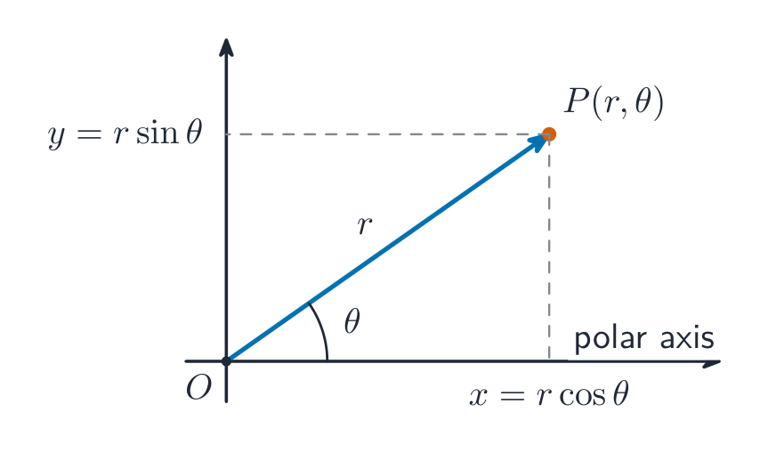
極座標は原点からの距離 $r$ と角度 $\theta$ によって点を表す。デカルト座標との関係は以下の通りである。
$$x = r\cos\theta, \qquad y = r\sin\theta, \qquad r^2 = x^2 + y^2.$$
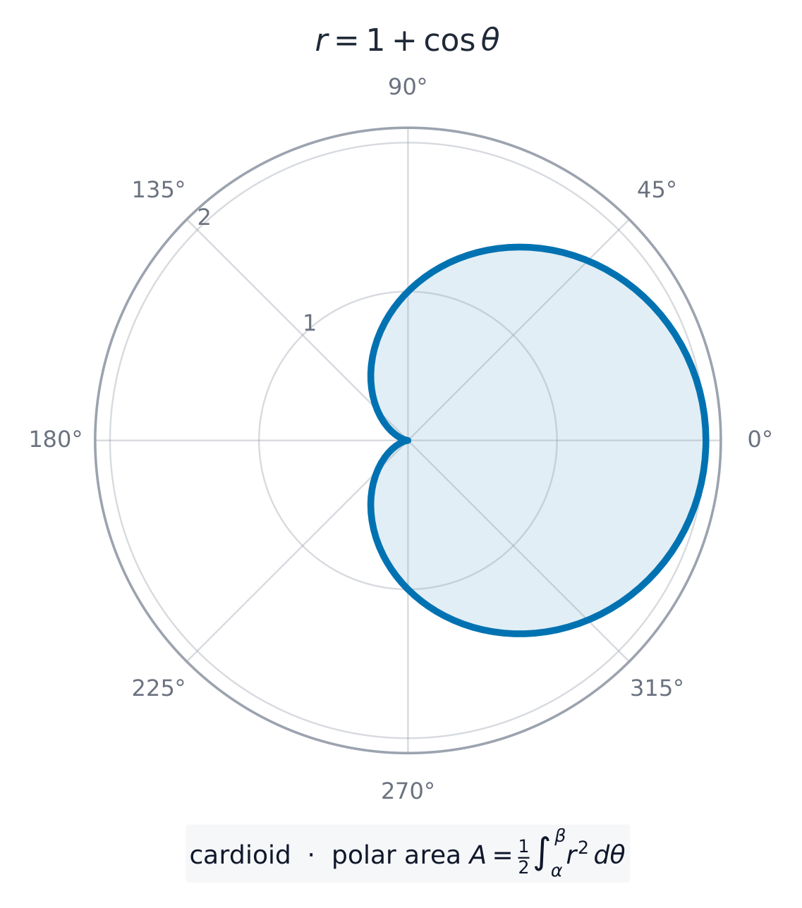
簡単な極曲線を描き、扇形の面積を求めるべきである。
$$\text{area} = \tfrac12\int r^2\,d\theta.$$
** worked example.** 極方程式 $r = 4\cos\theta$ をデカルト形式に変換せよ。
両辺に $r$ を掛けて $r^2 = 4r\cos\theta$ となるので、$x^2 + y^2 = 4x$ となる。平方完成すると $(x - 2)^2 + y^2 = 4$ となり、半径 $2$ で中心が $(2, 0)$ である円となる。
探索
極座標曲線
曲線を選択して a を変更する。極座標形式では点は距離 r と角度 θ で指定され、これによりバラ曲線、心形線、螺旋線が描かれる。
1.6
ベクトル

シラバス
| Candidates should be able to: | Notes and examples |
|---|---|
| use the equation of a plane in any of the forms $ax + by + cz = d$ or $\mathbf{r.n} = p$ or $\mathbf{r} = \mathbf{a} + \lambda\mathbf{b} + \mu\mathbf{c}$ and convert equations of planes from one form to another as necessary in solving problems | |
| recall that the vector product $\mathbf{a} \times \mathbf{b}$ of two vectors can be expressed either as $|\mathbf{a}||\mathbf{b}|\sin\theta\hat{\mathbf{n}}$, where $\hat{\mathbf{n}}$ is a unit vector, or in component form as $(a_2b_3 - a_3b_2)\mathbf{i} + (a_3b_1 - a_1b_3)\mathbf{j} + (a_1b_2 - a_2b_1)\mathbf{k}$ | |
| use equations of lines and planes, together with scalar and vector products where appropriate, to solve problems concerning distances, angles and intersections, including: – determining whether a line lies in a plane, is parallel to a plane or intersects a plane, and finding the point of intersection of a line and a plane when it exists – finding the foot of the perpendicular from a point to a plane – finding the angle between a line and a plane, and the angle between two planes – finding an equation for the line of intersection of two planes – calculating the shortest distance between two skew lines – finding an equation for the common perpendicular to two skew lines. |
出典: Cambridge International シラバス
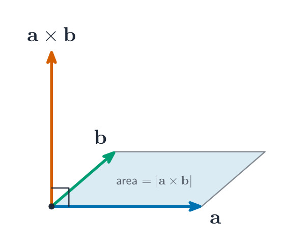
三次元空間において、平面は $ax + by + cz = d$ 、または $\mathbf{r}\cdot\mathbf{n} = p$ 、または $\mathbf{r} = \mathbf{a} + \lambda\mathbf{b} + \mu\mathbf{c}$ と表せる。内積他に、二つのベクトルの外積がある。
$$\mathbf{a}\times\mathbf{b} = |\mathbf{a}|\,|\mathbf{b}|\sin\theta\;\hat{\mathbf{n}},$$
これにより、両方のベクトルに垂直なベクトルが得られる。内積と外积を用いることで、距離、角度、直線と平面の交点(ねじれ直線間の最短距離を含む)を求めることができる。
** worked example(演習例)**。$\mathbf{a}\times\mathbf{b}$ を$\mathbf{a} = \mathbf{i} + \mathbf{j}$ および$\mathbf{b} = \mathbf{j} + \mathbf{k}$ について求めよ。
$$\mathbf{a}\times\mathbf{b} = \begin{vmatrix} \mathbf{i} & \mathbf{j} & \mathbf{k} \\ 1 & 1 & 0 \\ 0 & 1 & 1 \end{vmatrix} = \mathbf{i}(1) - \mathbf{j}(1) + \mathbf{k}(1) = \mathbf{i} - \mathbf{j} + \mathbf{k}。$$
探索
ベクトル
a · b = |a||b|cos θ
内積 がゼロになるのは、2つのベクトルが直交しているちょうどそのときである。
語彙
練習する
| English | 日本語 |
|---|---|
| vector product/ˈvektə ˈprɒdʌkt/ | ベクトル積 |
| vectors/ˈvektəz/ | ベクトル |
| skew lines/skjuː laɪnz/ | 異面直線 |
| mathematical induction/ˌmæθɪˈmætɪkl ɪnˈdʌkʃn/ | 数学的帰納法 |
| conjecture/kənˈdʒektʃə/ | 仮説 |
| inductive proof/ɪnˈdʌktɪv pruːf/ | 帰納法 |
| symmetric functions/sɪˈmetrɪk ˈfʌŋkʃnz/ | 対称関数 |
| discriminant/dɪˈskrɪmɪnənt/ | 判別式 |
| turning points/ˈtɜːnɪŋ pɔɪnts/ | 反転点 |
| partial fractions/ˈpɑːʃl ˈfrækʃnz/ | 部分分数分解 |
| rotation/rəʊˈteɪʃn/ | 回転 |
| reflection/rɪˈflekʃn/ | 反射 |
| enlargement/enˈlɑːdʒmənt/ | 拡大 |
| stretch/stretʃ/ | 伸縮 |
| shear/ʃɪə/ | せん断変形 |
1.7
帰納法による証明

シラバス
| Candidates should be able to: | Notes and examples |
|---|---|
| use the method of mathematical induction to establish a given result | e.g. $\sum_{r=1}^{n} r^4 = \frac{1}{4}n^2(n+1)^2$, $u_n = \frac{1}{2}(1 + 3^{n-1})$ for the sequence given by $u_{n+1} = 3u_n - 1$ and $u_1 = 1$, $\begin{pmatrix} 4 & -1 \\ 6 & -1 \end{pmatrix}^n = \begin{pmatrix} 3 \times 2^n - 2 & 1 - 2^n \\ 3 \times 2^{n+1} - 6 & 3 - 2^{n+1} \end{pmatrix}$, $3^{2n} + 2 \times 5^n - 3$ is divisible by 8. |
| recognise situations where conjecture based on a limited trial followed by inductive proof is a useful strategy, and carry this out in simple cases. | e.g. find the $n$th derivative of $x e^x$, find $\sum_{r=1}^{n} r \times r!$. |
出典: Cambridge International シラバス
数学的帰納法は、正の整数 $n$ すべてについてある命題が成り立つことを二つのステップで証明する手法である。
- 帰納の基礎: $n = 1$ に対して命題が真であることを示す。
- 帰納的步骤: $n = k$ に対して命題が真であると仮定し、$n = k + 1$ に対して成り立つことを証明する。
両方のステップが成立すれば、命題は全ての $n$ に対して真となる。多くの場合、まずいくつかのケースから推測(妥当な予想)を立て、次に帰納的证明によって確認する。
** worked example.** $\displaystyle\sum_{r=1}^{n} r = \tfrac12 n(n+1)$ が成り立つことを証明せよ。
帰納の基礎 $n = 1$ :左辺は $1$ 、右辺は $\tfrac12(1)(2) = 1$ 。真である。 帰納的ステップ: $\displaystyle\sum_{r=1}^{k} r = \tfrac12 k(k+1)$ が成り立つと仮定する。すると
$$\sum_{r=1}^{k+1} r = \tfrac12 k(k+1) + (k+1) = (k+1)\left(\tfrac{k}{2} + 1\right) = \tfrac12 (k+1)(k+2).$$
これは $n = k + 1$ を代入した公式なので、帰納法により全ての $n$ について成立する。
探索
帰納法による証明のプロセス
帰納法を、最初のドミノ再加上すべての次のケースを押すルールと捉える。
1.7
試験対策
- 多項式を解く代わりに、根と係数の関係(和、ペアごとの和、積)を用いる。
- 帰納法による証明では、帰納の基礎を設定し、$n = k$ に対して真であると仮定し、$n = k+1$ について証明し、明確な結びの言葉を記述する。
- 有理関数のグラフをその漸近線や極値点とともに描き、差分法を用いて級数の和を求める。
- 行列については、行列式、逆行列、不変直線を知り、各変換を幾何学的に解釈する。
このトピックのインタラクティブ授業
一歩ずつ進め、即時チェック付きの問題で学習します。