This handout covers Topic 1: Further Pure Mathematics 进阶纯数学 1. It adds new algebra, matrices, polar coordinates, more vectors, and proof by induction.
Tips · Советы
A-Level Further Mathematics (9231) sits on top of 9709 and assumes it: Further Pure 1 and 2, Further Mechanics, and Further Probability & Statistics. It is taken alongside Maths, not instead of it, and which components you sit depends on your school's entry.
Further Pure holds most of the new machinery — matrices and linear transformations, complex numbers in polar and exponential form, polar curves, hyperbolic functions, differential equations, proof by induction. This is genuinely new content, not harder versions of familiar content.
The realistic difficulty is time, not ideas. The algebra is long enough that an error in line two survives to the end, so write the method out fully and check at the halfway point.
-
1
Further Pure Mathematics 1 · Дополнительная чистая математика 1
Watch lesson · Смотреть урок1.1
Roots of polynomial equations
Syllabus · Программа
EnglishCandidates should be able to: Notes and examples • recall and use the relations between the roots and coefficients of polynomial equations e.g. to evaluate symmetric functions of the roots or to solve problems involving unknown coefficients in equations; restricted to equations of degree 2, 3 or 4 only. • use a substitution to obtain an equation whose roots are related in a simple way to those of the original equation Substitutions will not be given for the easiest cases, e.g. where the new roots are reciprocals or squares or a simple linear function of the old roots. РусскийКандидаты должны уметь: Примечания и примеры • вспомнить и использовать связи между корнями и коэффициентами полиномиальных уравнений например, для вычисления симметричных функций корней или решения задач с неизвестными коэффициентами в уравнениях; ограничено уравнениями только 2-й, 3-й или 4-й степени. • использовать замену переменной для получения уравнения, корни которого связаны простым образом с корнями исходного уравнения Замены не будут даны для простейших случаев, например, когда новые корни являются обратными величинами или квадратами или простой линейной функцией старых корней. Source: Cambridge International syllabus · Источник: Программа Cambridge International
For a polynomial equation, the roots 根 are linked to the coefficients 系数. For $ax^2 + bx + c = 0$ with roots $\alpha, \beta$:
$$\alpha + \beta = -\frac{b}{a}, \qquad \alpha\beta = \frac{c}{a}.$$For a cubic $ax^3 + bx^2 + cx + d = 0$ with roots $\alpha, \beta, \gamma$:$$\sum\alpha = -\frac{b}{a}, \qquad \sum\alpha\beta = \frac{c}{a}, \qquad \alpha\beta\gamma = -\frac{d}{a}.$$Sums like $\sum\alpha$ and $\sum\alpha\beta$ are symmetric functions 对称函数 of the roots (unchanged if the roots are swapped). To find an equation whose roots are changed in a simple way, use a substitution 代换 (for example, put $w = \alpha + 1$).Worked example. The equation $x^2 - 5x + 6 = 0$ has roots $\alpha, \beta$. Find the equation with roots $\alpha + 1, \beta + 1$.
Here $\alpha + \beta = 5$ and $\alpha\beta = 6$. The new sum is $(\alpha + 1) + (\beta + 1) = 7$, and the new product is $(\alpha + 1)(\beta + 1) = \alpha\beta + \alpha + \beta + 1 = 6 + 5 + 1 = 12$. So the new equation is
$$x^2 - 7x + 12 = 0.$$Explore · ИсследоватьRoots of a polynomial · Корни многочлена
y = ax³ + bx² + cx + d
The roots are where the curve meets the x-axis — their sum and product link to the coefficients. · Корни — это точки пересечения графика с осью x — их сумма и произведение связаны с коэффициентами.
Vocabulary · Словарь Train · ТренироватьEnglish Русский Further Pure Mathematics/ˈfɜːðə pjʊə ˌmæθɪˈmætɪks/ Дополнительная чистая математика (Further Pure Mathematics) roots/ruːts/ корни coefficients/ˌkəʊɪˈfɪʃənts/ коэффициенты substitution/ˌsʌbstɪˈtjuːʃn/ замещение symmetric functions/sɪˈmetrɪk ˈfʌŋkʃnz/ симметрические функции 1.2
Rational functions and graphs

Syllabus · Программа
EnglishCandidates should be able to: Notes and examples • sketch graphs of simple rational functions, including the determination of oblique asymptotes, in cases where the degree of the numerator and the denominator are at most 2 Including determination of the set of values taken by the function, e.g. by the use of a discriminant. Detailed plotting of curves will not be required, but sketches will generally be expected to show significant features, such as turning points, asymptotes and intersections with the axes. • understand and use relationships between the graphs of $y = f(x)$, $y^2 = f(x)$, $y = \frac{1}{f(x)}$, $y = |f(x)|$ and $y = f(|x|)$ Including use of such sketch graphs in the course of solving equations or inequalities. РусскийКандидаты должны уметь: Примечания и примеры • набрасывать эскизы графиков простых рациональных функций, включая определение наклонных асимптот, в случаях, когда степень числителя и знаменателя не превышает 2 Включая определение множества значений, принимаемых функцией, например, с помощью дискриминанта. Детальное построение кривых не требуется, но эскизы обычно должны показывать значимые особенности, такие как точки экстремума, асимптоты и пересечения с осями координат. • понимать и использовать взаимосвязи между графиками $y = f(x)$, $y^2 = f(x)$, $y = \frac{1}{f(x)}$, $y = |f(x)|$ и $y = f(|x|)$ Включая использование таких эскизов при решении уравнений или неравенств. Source: Cambridge International syllabus · Источник: Программа Cambridge International
A rational function 有理函数 is a fraction of two polynomials. When the top has degree exactly one higher than the bottom, the graph has an oblique asymptote 斜渐近线 (a slanted line the curve approaches); find it by dividing out. You should also be able to relate the graph of $y = f(x)$ to those of $y^2 = f(x)$, $y = \dfrac{1}{f(x)}$, $y = |f(x)|$ and $y = f(|x|)$. Find the set of values the function can take using the discriminant 判别式, and locate its turning points 驻点.
Far from the origin the curve hugs the slant line $y=x$; near $x=0$ it runs off along the vertical asymptote. Worked example. Find the oblique asymptote of $y = \dfrac{x^2 + x + 1}{x + 1}$.
Divide out the fraction: $\dfrac{x^2 + x + 1}{x + 1} = x + \dfrac{1}{x + 1}$. As $x \to \pm\infty$ the remainder $\dfrac{1}{x+1} \to 0$, so the curve approaches the line $y = x$ — the oblique asymptote.
Explore · ИсследоватьRational functions · Рациональные функции
y = a/(x − b) + c
A rational function has asymptotes the curve approaches but never touches. · У рациональной функции есть асимптоты — линии, к которым график приближается, но никогда не касается.
Vocabulary · Словарь Train · ТренироватьEnglish Русский rational function/ˈræʃənl ˈfʌŋkʃn/ рациональная функция oblique asymptote/əˈbliːk ˈæsɪmptəʊt/ наклонная асимптота discriminant/dɪˈskrɪmɪnənt/ дискриминант turning points/ˈtɜːnɪŋ pɔɪnts/ точки разворота 1.3
Summation of series
Syllabus · Программа
EnglishCandidates should be able to: Notes and examples • use the standard results for $\sum r$, $\sum r^2$, $\sum r^3$ to find related sums • use the method of differences to obtain the sum of a finite series Use of partial fractions to express a general term in a suitable form may be required. • recognise, by direct consideration of a sum to $n$ terms, when a series is convergent, and find the sum to infinity in such cases РусскийКандидаты должны уметь: Примечания и примеры • использовать стандартные результаты для $\sum r$, $\sum r^2$, $\sum r^3$ для нахождения связанных сумм • использовать метод телескопических сумм (метод разностей) для получения суммы конечного ряда Может потребоваться использование дробей на частные для представления общего члена в подходящей форме. • распознавать, рассматривая сумму $n$ членов, сходимость ряда и находить сумму бесконечного ряда в таких случаях Source: Cambridge International syllabus · Источник: Программа Cambridge International
Learn the standard results:
$$\sum_{r=1}^{n} r = \tfrac12 n(n+1), \qquad \sum_{r=1}^{n} r^2 = \tfrac16 n(n+1)(2n+1), \qquad \sum_{r=1}^{n} r^3 = \tfrac14 n^2(n+1)^2.$$The method of differences 差分法 sums a series by cancelling middle terms: if partial fractions 部分分式 write each term as $f(r) - f(r+1)$, almost everything cancels. From the sum to $n$ terms you can see whether a series is convergent 收敛 and, if so, find its sum to infinity 无穷和.Worked example. Find $\displaystyle\sum_{r=1}^{n} (2r + 1)$.
$$\sum_{r=1}^{n}(2r + 1) = 2\sum_{r=1}^{n} r + \sum_{r=1}^{n} 1 = 2\cdot\tfrac12 n(n+1) + n = n(n+1) + n = n(n+2).$$Explore · ИсследоватьSequences and their sums · Последовательности и их суммы
Step through the terms and the running total — the idea behind a series and its sum to n terms. · Проходите по членам и накопленной сумме — идея, стоящая за рядом и его суммой до n членов.
Vocabulary · Словарь Train · ТренироватьEnglish Русский method of differences/ˈmeθəd ɒv ˈdɪfrənsɪz/ метод разностей convergent/kənˈvɜːdʒənt/ конвергентный sum to infinity/sʌm tʊ ɪnˈfɪnɪti/ сумма бесконечного ряда partial fractions/ˈpɑːʃl ˈfrækʃnz/ разложения на простейшие дроби 1.4
Matrices

Syllabus · Программа
EnglishCandidates should be able to: Notes and examples carry out operations of matrix addition, subtraction and multiplication, and recognise the terms zero matrix and identity (or unit) matrix Including non-square matrices. Matrices will have at most 3 rows and columns. recall the meaning of the terms singular and non-singular as applied to square matrices and, for $2 \times 2$ and $3 \times 3$ matrices, evaluate determinants and find inverses of non-singular matrices The notations $\det \mathbf{M}$ for the determinant of a matrix $\mathbf{M}$, and $\mathbf{I}$ for the identity matrix, will be used. understand and use the result, for non-singular matrices, $(\mathbf{AB})^{-1} = \mathbf{B}^{-1}\mathbf{A}^{-1}$ Extension to the product of more than two matrices may be required. understand the use of $2 \times 2$ matrices to represent certain geometric transformations in the $x$-$y$ plane, in particular: – understand the relationship between the transformations represented by $\mathbf{A}$ and $\mathbf{A}^{-1}$ – recognise that the matrix product $\mathbf{AB}$ represents the transformation that results from the transformation represented by $\mathbf{B}$ followed by the transformation represented by $\mathbf{A}$ – recall how the area scale factor of a transformation is related to the determinant of the corresponding matrix – find the matrix that represents a given transformation or sequence of transformations Understanding of the terms rotation, reflection, enlargement, stretch and shear for 2D transformations will be required. Other 2D transformations may be included, but no particular knowledge of them is expected. understand the meaning of invariant as applied to points and lines in the context of transformations represented by matrices, and solve simple problems involving invariant points and invariant lines. e.g. to locate the invariant points of the transformation represented by $\begin{pmatrix} 6 & 5 \\ 2 & 3 \end{pmatrix}$, or to find the invariant lines through the origin for $\begin{pmatrix} 4 & -1 \\ 2 & 1 \end{pmatrix}$, or to show that any line with gradient 1 is invariant for $\begin{pmatrix} 2 & 0 \\ 1 & 1 \end{pmatrix}$. РусскийКандидаты должны уметь: Примечания и примеры выполнять операции сложения матриц, вычитания и умножения, а также распознавать понятия нулевая матрица и единичная (или тождественная) матрица Включая неквадратные матрицы. Число строк и столбцов матриц — не более 3. вспомнить значения терминов вырожденный и невывожденный применительно к квадратным матрицам и для матриц размера $2 \times 2$ и $3 \times 3$ вычислять определители и находить обратные матрицы для невырожденных матриц Будут использоваться обозначения $\det \mathbf{M}$ для определителя матрицы $\mathbf{M}$ и $\mathbf{I}$ для единичной матрицы. понимать и использовать результат для невырожденных матриц: $(\mathbf{AB})^{-1} = \mathbf{B}^{-1}\mathbf{A}^{-1}$ Может потребоваться обобщение на произведение более двух матриц. понимать использование матриц $2 \times 2$ для представления определённых геометрических преобразований в плоскости $x$-$y$, в частности: – понять связь между преобразованиями, представленными матрицами $\mathbf{A}$ и $\mathbf{A}^{-1}$ – распознать, что произведение матриц $\mathbf{AB}$ представляет преобразование, resulting from (результатом) преобразования, представленного матрицей $\mathbf{B}$, за которым следует преобразование, представленное матрицей $\mathbf{A}$ – вспомнить, как масштабный коэффициент площади преобразования связан с определителем соответствующей матрицы – найти матрицу, представляющую заданное преобразование или последовательность преобразований Понимание терминов поворот, отражение, увеличение, растяжение и сдвиг для преобразований 2 будет необходимо. Другие преобразования 2 могут быть включены, но специальные знания о них не требуются. понимать значение термина инвариантный применительно к точкам и прямым в контексте преобразований, задаваемых матрицами, и решать простые задачи, связанные с инвариантными точками и инвариантными прямыми. Например: найти инвариантные точки преобразования, заданного матрицей $\begin{pmatrix} 6 & 5 \\ 2 & 3 \end{pmatrix}$; найти инвариантные прямые, проходящие через начало координат, для матрицы $\begin{pmatrix} 4 & -1 \\ 2 & 1 \end{pmatrix}$; доказать, что любая прямая с угловым коэффициентом 1 является инвариантной для матрицы $\begin{pmatrix} 2 & 0 \\ 1 & 1 \end{pmatrix}$. Source: Cambridge International syllabus · Источник: Программа Cambridge International
A matrix moves the plane A matrix 矩阵 is a rectangular block of numbers. Matrix addition adds entries in matching positions; you can also subtract and multiply matrices (multiplication is row $\times$ column). The zero matrix 零矩阵 has every entry $0$, and the identity matrix 单位矩阵 (or unit matrix) $I$ leaves any matrix unchanged under multiplication.
For a $2\times 2$ matrix $A = \begin{pmatrix} a & b \\ c & d \end{pmatrix}$, the determinant 行列式 is $\det A = ad - bc$. If $\det A \neq 0$ the matrix is non-singular (otherwise it is a singular matrix 奇异矩阵), and the inverse matrix 逆矩阵 is
$$A^{-1} = \frac{1}{ad - bc}\begin{pmatrix} d & -b \\ -c & a \end{pmatrix}.$$For a product, $(AB)^{-1} = B^{-1}A^{-1}$. A $2\times 2$ matrix can represent a geometric transformation 几何变换 of the plane — a rotation 旋转, reflection 反射, enlargement 放大, stretch 拉伸 or shear 切变: the determinant gives the area scale factor, and a product $AB$ means "do $B$, then $A$". Points or lines that do not move are called invariant points 不变点 and invariant lines 不变直线.The matrix sends the unit square to a parallelogram whose area is the determinant. Worked example. Find the inverse of $A = \begin{pmatrix} 3 & 1 \\ 2 & 4 \end{pmatrix}$.
$\det A = 3\times 4 - 1\times 2 = 10$, so
$$A^{-1} = \frac{1}{10}\begin{pmatrix} 4 & -1 \\ -2 & 3 \end{pmatrix}.$$Explore · ИсследоватьMatrices as transformations · Матрицы как преобразования
Change the four entries and watch the unit square map to a new shape. The determinant is the area scale factor. · Измените четыре элемента и наблюдайте, как единичный квадрат отображается в новую форму. Определитель является множителем масштаба площади.
Vocabulary · Словарь Train · ТренироватьEnglish Русский matrix/ˈmeɪtrɪks/ матричной zero matrix/ˈzɪərəʊ ˈmeɪtrɪks/ нулевая матрица identity matrix/aɪˈdentɪti ˈmeɪtrɪks/ единичная матрица determinant/dɪˈtɜːmɪnənt/ определитель singular matrix/ˈsɪŋɡjʊlə ˈmeɪtrɪks/ вырожденная матрица inverse matrix/ɪnˈvɜːs ˈmeɪtrɪks/ обратная матрица geometric transformation/ˌdʒiːəʊˈmetrɪk trænsfɔːˈmeɪʃn/ геометрическое преобразование invariant points/ɪnˈveərɪənt pɔɪnts/ инвариантные точки invariant lines/ɪnˈveərɪənt laɪnz/ инвариантные прямые rotation/rəʊˈteɪʃn/ поворот reflection/rɪˈflekʃn/ отражения enlargement/enˈlɑːdʒmənt/ увеличение stretch/stretʃ/ растяжением shear/ʃɪə/ сдвиг 1.5
Polar coordinates

Syllabus · Программа
EnglishCandidates should be able to: Notes and examples understand the relations between Cartesian and polar coordinates, and convert equations of curves from Cartesian to polar form and vice versa The convention $r \geqslant 0$ will be used. sketch simple polar curves, for $0 \leqslant \theta < 2\pi$ or $-\pi < \theta \leqslant \pi$ or a subset of either of these intervals Detailed plotting of curves will not be required, but sketches will generally be expected to show significant features, such as symmetry, coordinates of intersections with the initial line, the form of the curve at the pole and least/greatest values of $r$. recall the formula $\frac{1}{2} \int r^2 \mathrm{d}\theta$ for the area of a sector, and use this formula in simple cases. РусскийКандидаты должны уметь: Примечания и примеры понимать соотношения между декартовыми и полярными координатами и преобразовывать уравнения кривых из декартовой формы в полярную и обратно Будет использоваться конвенция $r \geqslant 0$. строить эскизы простых полярных кривых для интервалов $0 \leqslant \theta < 2\pi$ или $-\pi < \theta \leqslant \pi$ или подмножеств этих интервалов Детальное построение графиков не требуется, но эскизы обычно должны отображать существенные особенности, такие как симметрия, координаты пересечения с начальной прямой, поведение кривой у полюса, а также наименьшие/наибольшие значения $r$. вспомнить формулу $\frac{1}{2} \int r^2 \mathrm{d}\theta$ для площади сектора и применять её в простых случаях. Source: Cambridge International syllabus · Источник: Программа Cambridge International
Tracing a polar curve: the cardioid A spiral staircase: spirals are described naturally using polar coordinates. Polar coordinates 极坐标 give a point by its distance $r$ from the origin and its angle $\theta$. They link to Cartesian coordinates 直角坐标 by
$$x = r\cos\theta, \qquad y = r\sin\theta, \qquad r^2 = x^2 + y^2.$$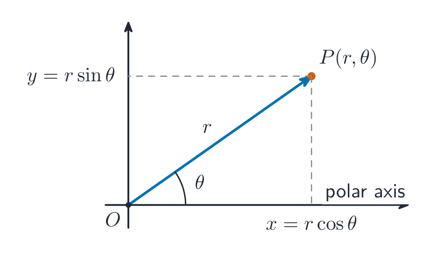
Polar coordinates $(r,\theta)$ convert to Cartesian by $x=r\cos\theta$ and $y=r\sin\theta$. You should sketch simple polar curves 极坐标曲线, and find the area of a sector with
$$\text{area} = \tfrac12\int r^2\,d\theta.$$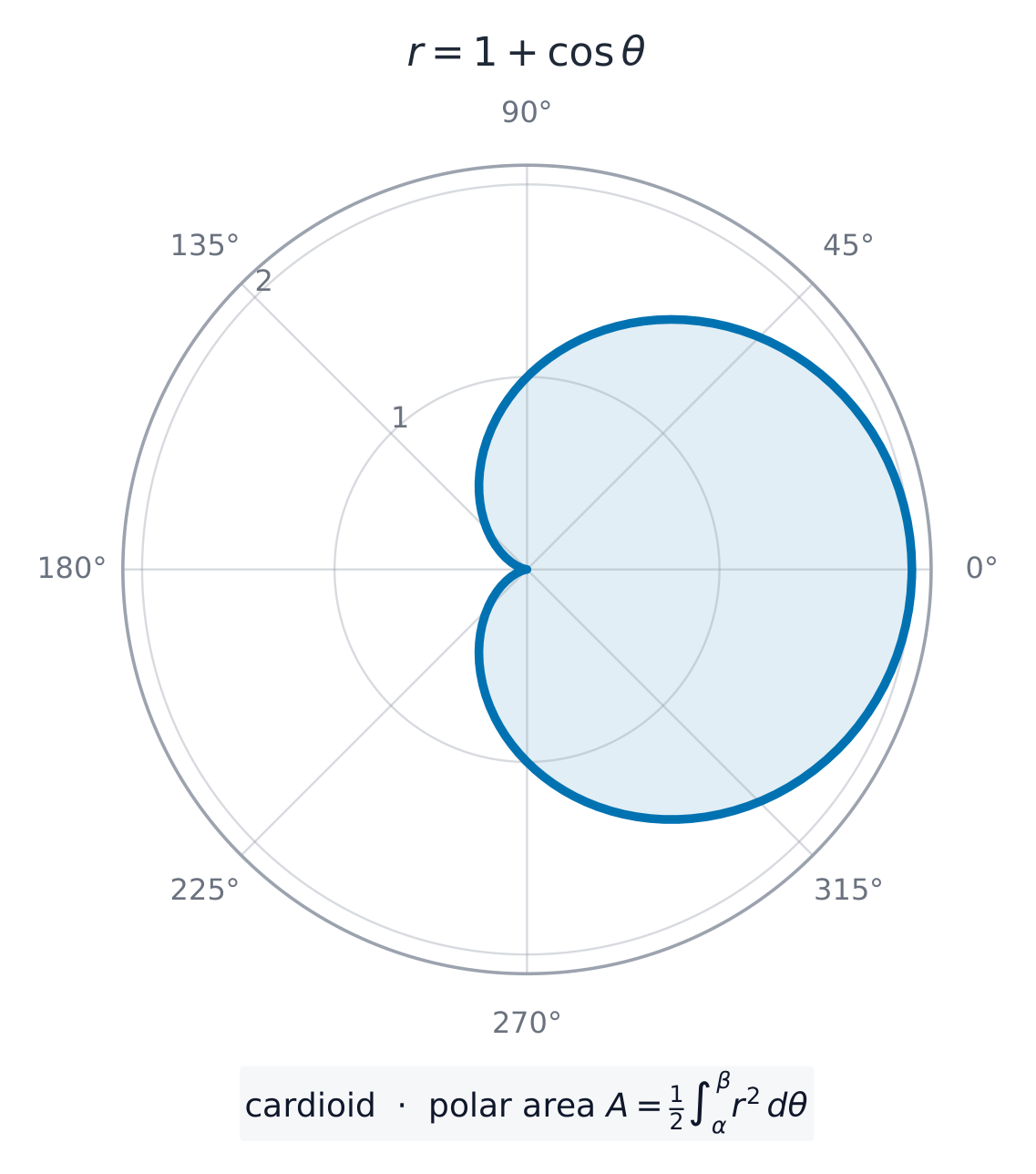
The cardioid $r=1+\cos\theta$, plotted straight from $r$ as a function of $\theta$. Worked example. Convert the polar equation $r = 4\cos\theta$ to Cartesian form.
Multiply both sides by $r$: $r^2 = 4r\cos\theta$, so $x^2 + y^2 = 4x$. Completing the square gives $(x - 2)^2 + y^2 = 4$, a circle of radius $2$ centred at $(2, 0)$.
Explore · ИсследоватьPolar curves · Полярные кривые
Pick a curve and change a. In polar form a point is set by its distance r and angle θ — that draws roses, cardioids and spirals. · Выберите кривую и измените a. В полярной форме точка задается расстоянием r и углом θ — так рисуются розы, кардиоиды и спирали.
Vocabulary · Словарь Train · ТренироватьEnglish Русский polar coordinates/ˈpəʊlə kəʊˈɔːdɪnəts/ полярные координаты Cartesian coordinates/kɑːˈtiːzɪən kəʊˈɔːdɪnəts/ декартовы координаты polar curves/ˈpəʊlə kɜːvz/ полярные кривые 1.6
Vectors

Syllabus · Программа
EnglishCandidates should be able to: Notes and examples use the equation of a plane in any of the forms $ax + by + cz = d$ or $\mathbf{r.n} = p$ or $\mathbf{r} = \mathbf{a} + \lambda\mathbf{b} + \mu\mathbf{c}$ and convert equations of planes from one form to another as necessary in solving problems recall that the vector product $\mathbf{a} \times \mathbf{b}$ of two vectors can be expressed either as $|\mathbf{a}||\mathbf{b}|\sin\theta\hat{\mathbf{n}}$, where $\hat{\mathbf{n}}$ is a unit vector, or in component form as $(a_2b_3 - a_3b_2)\mathbf{i} + (a_3b_1 - a_1b_3)\mathbf{j} + (a_1b_2 - a_2b_1)\mathbf{k}$ use equations of lines and planes, together with scalar and vector products where appropriate, to solve problems concerning distances, angles and intersections, including: – determining whether a line lies in a plane, is parallel to a plane or intersects a plane, and finding the point of intersection of a line and a plane when it exists – finding the foot of the perpendicular from a point to a plane – finding the angle between a line and a plane, and the angle between two planes – finding an equation for the line of intersection of two planes – calculating the shortest distance between two skew lines – finding an equation for the common perpendicular to two skew lines. РусскийКандидаты должны уметь: Примечания и примеры Использовать уравнение плоскости в любой из форм $ax + by + cz = d$ или $\mathbf{r.n} = p$ или $\mathbf{r} = \mathbf{a} + \lambda\mathbf{b} + \mu\mathbf{c}$ и преобразовывать уравнения плоскостей из одной формы в другую при необходимости решения задач вспомнить, что векторное произведение $\mathbf{a} \times \mathbf{b}$ двух векторов может быть выражено либо как $|\mathbf{a}||\mathbf{b}|\sin\theta\hat{\mathbf{n}}$, где $\hat{\mathbf{n}}$ — единичный вектор, либо в компонентной форме как $(a_2b_3 - a_3b_2)\mathbf{i} + (a_3b_1 - a_1b_3)\mathbf{j} + (a_1b_2 - a_2b_1)\mathbf{k}$ использовать уравнения прямых и плоскостей, а также скалярное и векторное произведения (где это уместно), для решения задач, связанных с расстояниями, углами и пересечениями, включая: – определение того, лежит ли прямая в плоскости, параллельна ей или пересекает её, и нахождение точки пересечения прямой и плоскости, если она существует – нахождение основания перпендикуляра, опущенного из точки на плоскость – нахождение угла между прямой и плоскостью, а также угла между двумя плоскостями – нахождение уравнения прямой пересечения двух плоскостей – вычисление кратчайшего расстояния между двумя скрещивающимися прямыми – нахождение уравнения общего перпендикуляра к двум скрещивающимся прямым. Source: Cambridge International syllabus · Источник: Программа Cambridge International
Forces like wind and water are vectors — they have both size and direction. In three dimensions a plane 平面 can be written as $ax + by + cz = d$, or $\mathbf{r}\cdot\mathbf{n} = p$, or $\mathbf{r} = \mathbf{a} + \lambda\mathbf{b} + \mu\mathbf{c}$. Besides the scalar product, there is the vector product 向量积 of two vectors 向量:
$$\mathbf{a}\times\mathbf{b} = |\mathbf{a}|\,|\mathbf{b}|\sin\theta\;\hat{\mathbf{n}},$$which gives a vector at right angles to both. With scalar and vector products you can find distances, angles, and where lines and planes meet — including the shortest distance between skew lines 异面直线.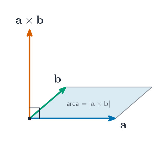
$\mathbf{a}\times\mathbf{b}$ is perpendicular to both vectors; its length equals the area of the parallelogram they span. Worked example. Find $\mathbf{a}\times\mathbf{b}$ for $\mathbf{a} = \mathbf{i} + \mathbf{j}$ and $\mathbf{b} = \mathbf{j} + \mathbf{k}$.
$$\mathbf{a}\times\mathbf{b} = \begin{vmatrix} \mathbf{i} & \mathbf{j} & \mathbf{k} \\ 1 & 1 & 0 \\ 0 & 1 & 1 \end{vmatrix} = \mathbf{i}(1) - \mathbf{j}(1) + \mathbf{k}(1) = \mathbf{i} - \mathbf{j} + \mathbf{k}.$$Explore · ИсследоватьVectors · Векторы
a · b = |a||b|cos θ
The dot product is zero exactly when two vectors are perpendicular. · Скалярное произведение равно нулю тогда и только тогда, когда два вектора перпендикулярны.
Vocabulary · Словарь Train · ТренироватьEnglish Русский plane/pleɪn/ плоскость vector product/ˈvektə ˈprɒdʌkt/ векторное произведение vectors/ˈvektəz/ векторы skew lines/skjuː laɪnz/ скрещивающиеся прямые 1.7
Proof by induction

Syllabus · Программа
EnglishCandidates should be able to: Notes and examples use the method of mathematical induction to establish a given result e.g. $\sum_{r=1}^{n} r^4 = \frac{1}{4}n^2(n+1)^2$, $u_n = \frac{1}{2}(1 + 3^{n-1})$ for the sequence given by $u_{n+1} = 3u_n - 1$ and $u_1 = 1$, $\begin{pmatrix} 4 & -1 \\ 6 & -1 \end{pmatrix}^n = \begin{pmatrix} 3 \times 2^n - 2 & 1 - 2^n \\ 3 \times 2^{n+1} - 6 & 3 - 2^{n+1} \end{pmatrix}$, $3^{2n} + 2 \times 5^n - 3$ is divisible by 8. recognise situations where conjecture based on a limited trial followed by inductive proof is a useful strategy, and carry this out in simple cases. e.g. find the $n$th derivative of $x e^x$, find $\sum_{r=1}^{n} r \times r!$. РусскийКандидаты должны уметь: Примечания и примеры использовать метод математической индукции для доказательства заданного результата Например: $\sum_{r=1}^{n} r^4 = \frac{1}{4}n^2(n+1)^2$, $u_n = \frac{1}{2}(1 + 3^{n-1})$ для последовательности, заданной $u_{n+1} = 3u_n - 1$, и $u_1 = 1$, $\begin{pmatrix} 4 & -1 \\ 6 & -1 \end{pmatrix}^n = \begin{pmatrix} 3 \times 2^n - 2 & 1 - 2^n \\ 3 \times 2^{n+1} - 6 & 3 - 2^{n+1} \end{pmatrix}$, $3^{2n} + 2 \times 5^n - 3$ делится на 8. распознавать ситуации, где гипотеза, основанная на ограниченном опыте, с последующим доказательством по индукции, является полезной стратегией, и реализовывать её в простых случаях. Например: найти $n$-ю производную от $x e^x$; найти $\sum_{r=1}^{n} r \times r!$. Source: Cambridge International syllabus · Источник: Программа Cambridge International
Induction: the domino proof Mathematical induction 数学归纳法 proves a result for every positive integer $n$ in two steps:
- Base case: show the result is true for $n = 1$.
- Inductive step: assume it is true for $n = k$, then prove it for $n = k + 1$.
If both steps work, the result is true for all $n$. Often you first make a conjecture 猜想 (a sensible guess) from a few cases, then confirm it by inductive proof 归纳证明.
Induction is like dominoes: the base case topples the first, and the inductive step makes each one knock over the next — so the result holds for every n Worked example. Prove that $\displaystyle\sum_{r=1}^{n} r = \tfrac12 n(n+1)$.
Base case $n = 1$: the left side is $1$ and the right side is $\tfrac12(1)(2) = 1$. True. Inductive step: assume $\displaystyle\sum_{r=1}^{k} r = \tfrac12 k(k+1)$. Then
$$\sum_{r=1}^{k+1} r = \tfrac12 k(k+1) + (k+1) = (k+1)\left(\tfrac{k}{2} + 1\right) = \tfrac12 (k+1)(k+2).$$This is the formula with $n = k + 1$, so by induction it holds for all $n$.Explore · ИсследоватьProof by induction route · Маршрут доказательства методом математической индукции
See induction as a first domino plus a rule that pushes every next case. · Представьте индукцию как первый падающий домино plus правило, толкающее каждый следующий случай.
Vocabulary · Словарь Train · ТренироватьEnglish Русский mathematical induction/ˌmæθɪˈmætɪkl ɪnˈdʌkʃn/ математическая индукция conjecture/kənˈdʒektʃə/ гипотеза inductive proof/ɪnˈdʌktɪv pruːf/ математическая индукция 1.7
Exam tips
- Use the relationships between roots and coefficients (sum, sum of pairs, product) instead of solving the polynomial.
- For proof by induction, set out the base case, assume the result for $n = k$, prove it for $n = k+1$, and write a clear closing statement.
- Sketch rational-function graphs with their asymptotes and turning points; use the method of differences for a summation.
- For matrices, know the determinant, inverse and invariant lines, and interpret each transformation geometrically.
-
2
Further Pure Mathematics 2 · Дополнительная чистая математика 2
Watch lesson · Смотреть урокThis handout covers Topic 2: Further Pure Mathematics 进阶纯数学 2. It adds hyperbolic functions, eigenvalues, new differentiation and integration, de Moivre's theorem, and methods for differential equations.
2.1
Hyperbolic functions

Syllabus · Программа
EnglishCandidates should be able to: Notes and examples understand the definitions of the hyperbolic functions $\sinh x$, $\cosh x$, $\tanh x$, $\text{sech } x$, $\text{cosech } x$, $\text{coth } x$ in terms of the exponential function sketch the graphs of hyperbolic functions prove and use identities involving hyperbolic functions e.g. $\cosh^2 x - \sinh^2 x \equiv 1$, $\sinh 2x \equiv 2 \sinh x \cosh x$, and similar results corresponding to the standard trigonometric identities. understand and use the definitions of the inverse hyperbolic functions and derive and use the logarithmic forms РусскийКандидаты должны уметь: Примечания и примеры понимать определения гиперболических функций $\sinh x$, $\cosh x$, $\tanh x$, $\text{sech } x$, $\text{cosech } x$, $\text{coth } x$ через экспоненциальную функцию строить графики гиперболических функций доказывать и использовать тождества,涉及的 гиперболическими функциями Например: $\cosh^2 x - \sinh^2 x \equiv 1$, $\sinh 2x \equiv 2 \sinh x \cosh x$, и аналогичные результаты, соответствующие стандартным тригонометрическим тождествам. понимать и использовать определения обратных гиперболических функций и выводить, а также использовать логарифмические формы Source: Cambridge International syllabus · Источник: Программа Cambridge International
cosh and sinh built from exponentials A hanging cable forms a catenary — the curve of the hyperbolic cosine. The hyperbolic functions 双曲函数 are built from the exponential function:
$$\cosh x = \frac{e^x + e^{-x}}{2}, \qquad \sinh x = \frac{e^x - e^{-x}}{2}, \qquad \tanh x = \frac{\sinh x}{\cosh x}.$$
$\cosh$ is the average of $e^x$ and $e^{-x}$; $\sinh$ is half their difference. They obey identities much like the trigonometric ones, the main one being $\cosh^2 x - \sinh^2 x = 1$. The three reciprocals complete the set: $\operatorname{sech} x = \dfrac{1}{\cosh x}$, $\operatorname{cosech} x = \dfrac{1}{\sinh x}$, and $\coth x = \dfrac{1}{\tanh x} = \dfrac{\cosh x}{\sinh x}$ – all built from $e^x$ too, and worth recognising in integrals and mark schemes. The inverse hyperbolic functions 反双曲函数 have a logarithmic form 对数形式, for example $\sinh^{-1} x = \ln\!\left(x + \sqrt{x^2 + 1}\right)$.
Worked example. Show that $\cosh^2 x - \sinh^2 x = 1$.
$$\cosh^2 x - \sinh^2 x = \frac{(e^x + e^{-x})^2 - (e^x - e^{-x})^2}{4} = \frac{(e^{2x} + 2 + e^{-2x}) - (e^{2x} - 2 + e^{-2x})}{4} = \frac{4}{4} = 1.$$Explore · ИсследоватьHyperbolic functions · Гиперболические функции
y = a cosh(x)
cosh is the catenary (a hanging chain) — even, with its minimum at (0, a). · cosh — это цепная линия (провисающая цепь) — четная функция, с минимумом в точке (0, a).
Vocabulary · Словарь Train · ТренироватьEnglish Русский Further Pure Mathematics/ˈfɜːðə pjʊə ˌmæθɪˈmætɪks/ Дополнительная чистая математика (Further Pure Mathematics) hyperbolic functions/ˌhaɪpəˈbɒlɪk ˈfʌŋkʃnz/ гиперболические функции inverse hyperbolic functions/ɪnˈvɜːs ˌhaɪpəˈbɒlɪk ˈfʌŋkʃnz/ обратные гиперболические функции logarithmic form/ˌlɒɡəˈrɪθmɪk fɔːm/ логарифмическая форма 2.2
Matrices

Syllabus · Программа
EnglishCandidates should be able to: Notes and examples formulate a problem involving the solution of 3 linear simultaneous equations in 3 unknowns as a problem involving the solution of a matrix equation, or vice versa understand the cases that may arise concerning the consistency or inconsistency of 3 linear simultaneous equations, relate them to the singularity or otherwise of the corresponding matrix, solve consistent systems, and interpret geometrically in terms of lines and planes e.g. three planes meeting in a common point, or in a common line, or having no common points. understand the terms 'characteristic equation', 'eigenvalue' and 'eigenvector', as applied to square matrices Including use of the definition $\mathbf{Ae} = \lambda \mathbf{e}$ to prove simple properties, e.g. that $\lambda^n$ is an eigenvalue of $\mathbf{A}^n$. find eigenvalues and eigenvectors of $2 \times 2$ and $3 \times 3$ matrices Restricted to cases where the eigenvalues are real and distinct. express a square matrix in the form $\mathbf{QDQ}^{-1}$, where $\mathbf{D}$ is a diagonal matrix of eigenvalues and $\mathbf{Q}$ is a matrix whose columns are eigenvectors, and use this expression e.g. in calculating powers of $2 \times 2$ or $3 \times 3$ matrices. use the fact that a square matrix satisfies its own characteristic equation. e.g. in finding successive powers of a matrix or finding an inverse matrix; restricted to $2 \times 2$ or $3 \times 3$ matrices only. РусскийКандидаты должны уметь: Примечания и примеры формулировать задачу, связанную с решением системы из 3 линейных одновременных уравнений с 3 неизвестными, как задачу о решении матричного уравнения, или наоборот понимать возможные случаи совместности или несовместности системы из 3 линейных одновременных уравнений, связывать их с вырожденностью или отсутствием таковой соответствующей матрицы, решать совместные системы и интерпретировать их геометрически в терминах прямых и плоскостей Например: три плоскости, пересекающиеся в общей точке, в общей прямой или не имеющие общих точек. понимать термины «характеристическое уравнение», «собственное число» и «собственный вектор» применительно к квадратным матрицам Включая использование определения $\mathbf{Ae} = \lambda \mathbf{e}$ для доказательства простых свойств, например, что $\lambda^n$ является собственным числом матрицы $\mathbf{A}^n$. найти собственные значения и собственные векторы матриц $2 \times 2$ и $3 \times 3$ Ограничено случаями, когда собственные значения вещественны и различны. представить квадратную матрицу в виде $\mathbf{QDQ}^{-1}$, где $\mathbf{D}$ — диагональная матрица собственных значений, а $\mathbf{Q}$ — матрица, столбцы которой являются собственными векторами, и использовать это представление напр., при вычислении степеней матриц $2 \times 2$ или $3 \times 3$. использовать тот факт, что квадратная матрица удовлетворяет своему характеристическому уравнению. напр., при нахождении последовательных степеней матрицы или обратной матрицы; ограничено матрицами $2 \times 2$ или $3 \times 3$ только. Source: Cambridge International syllabus · Источник: Программа Cambridge International
A matrix moves the plane You can write three linear equations in three unknowns as a single matrix equation 矩阵方程 $A\mathbf{x} = \mathbf{b}$. If $A$ is non-singular there is one solution; if $A$ is singular the equations are either inconsistent (no solution) or have infinitely many.
For a square matrix $A$, the characteristic equation 特征方程 is $\det(A - \lambda I) = 0$. Its solutions are the eigenvalues 特征值 $\lambda$, and for each one the vector $\mathbf{v}$ with $A\mathbf{v} = \lambda\mathbf{v}$ is an eigenvector 特征向量. You can then write $A = QDQ^{-1}$, where $D$ is a diagonal matrix 对角矩阵 of eigenvalues and the columns of $Q$ are the eigenvectors.
Multiplying an eigenvector by $A$ only stretches it; a general vector is turned to a new direction. Worked example. Find the eigenvalues of $A = \begin{pmatrix} 2 & 1 \\ 1 & 2 \end{pmatrix}$.
The characteristic equation is
$$\det\begin{pmatrix} 2 - \lambda & 1 \\ 1 & 2 - \lambda \end{pmatrix} = (2 - \lambda)^2 - 1 = 0 \;\Rightarrow\; 2 - \lambda = \pm 1.$$So $\lambda = 1$ or $\lambda = 3$. (The eigenvector for $\lambda = 3$ is $\begin{pmatrix} 1 \\ 1 \end{pmatrix}$ and for $\lambda = 1$ is $\begin{pmatrix} 1 \\ -1 \end{pmatrix}$.)Explore · ИсследоватьTransformations and the determinant · Преобразования и определитель
Change the matrix to rotate, stretch or shear the unit square; the determinant shows how area changes. · Измените матрицу, чтобы повернуть, растянуть или сдвинуть единичный квадрат; определитель показывает, как изменяется площадь.
Vocabulary · Словарь Train · ТренироватьEnglish Русский matrix equation/ˈmeɪtrɪks ɪˈkweɪʒn/ матричное уравнение characteristic equation/ˌkærɪktəˈrɪstɪk ɪˈkweɪʒn/ характеристическое уравнение eigenvalues/ˈaɪdʒənvæljuːz/ собственные значения eigenvector/ˈaɪdʒənvektə/ собственный вектор diagonal matrix/daɪˈæɡənl ˈmeɪtrɪks/ диагональная матрица 2.3
Differentiation

Syllabus · Программа
EnglishCandidates should be able to: Notes and examples • differentiate hyperbolic functions and differentiate $\sin^{-1}x$, $\cos^{-1}x$, $\sinh^{-1}x$, $\cosh^{-1}x$ and $\tanh^{-1}x$ • obtain an expression for $\frac{\text{d}^2y}{\text{d}x^2}$ in cases where the relation between $x$ and $y$ is defined implicitly or parametrically • derive and use the first few terms of a Maclaurin's series for a function. Derivation of a general term is not included, but successive 'implicit' differentiation steps may be required, e.g. for $y = \tan x$ following an initial differentiation rearranged as $y' = 1 + y^2$. РусскийКандидаты должны уметь: Примечания и примеры • дифференцировать гиперболические функции и дифференцировать $\sin^{-1}x$, $\cos^{-1}x$, $\sinh^{-1}x$, $\cosh^{-1}x$ и $\tanh^{-1}x$ • получить выражение для $\frac{\text{d}^2y}{\text{d}x^2}$ в случаях, когда зависимость между $x$ и $y$ задана неявно или параметрически • вывести и использовать первые несколько членов ряда Маклорена для функции. Вывод общего члена не включен, но могут потребоваться последовательные шаги «неявного» дифференцирования, напр., для $y = \tan x$ после начального дифференцирования, преобразованного как $y' = 1 + y^2$. Source: Cambridge International syllabus · Источник: Программа Cambridge International
You can now differentiate the hyperbolic functions and the inverse functions $\sin^{-1}x$, $\tan^{-1}x$, $\sinh^{-1}x$ and so on. You can also find $\dfrac{d^2y}{dx^2}$ for curves given implicitly or parametrically.
A Maclaurin's series 麦克劳林级数 writes a function as a power series:
$$f(x) = f(0) + f'(0)\,x + \frac{f''(0)}{2!}\,x^2 + \frac{f'''(0)}{3!}\,x^3 + \cdots$$For example $e^x = 1 + x + \dfrac{x^2}{2!} + \dfrac{x^3}{3!} + \cdots$Adding more terms makes the polynomial match $e^x$ over a wider stretch around $x=0$. Worked example. Find the Maclaurin series of $f(x) = \ln(1+x)$ up to the term in $x^3$.
$f(0) = 0$; $f'(x) = \dfrac{1}{1+x}$ so $f'(0) = 1$; $f''(x) = \dfrac{-1}{(1+x)^2}$ so $f''(0) = -1$; $f'''(x) = \dfrac{2}{(1+x)^3}$ so $f'''(0) = 2$. Substituting into the series:
$$\ln(1+x) = x - \frac{x^2}{2} + \frac{x^3}{3} - \cdots$$Explore · ИсследоватьThe gradient at a point · Наклон касательной в точке
gradient = dy/dx · наклон = dy/dx
The derivative is the slope of the tangent, however exotic the function. · Производная — это наклон касательной, какой бы экзотической ни была функция.
Vocabulary · Словарь Train · ТренироватьEnglish Русский Maclaurin's series/məˈklɔːrɪnz ˈsɪəriːz/ ряд Маклорена 2.4
Integration
Syllabus · Программа
EnglishCandidates should be able to: Notes and examples • integrate hyperbolic functions and recognise integrals of functions of the form $\frac{1}{\sqrt{a^2 - x^2}}$, $\frac{1}{\sqrt{x^2 + a^2}}$ and $\frac{1}{\sqrt{x^2 - a^2}}$, and integrate associated functions using trigonometric substitutions or hyperbolic substitutions as appropriate Including use of completing the square where necessary, e.g. to integrate $\frac{1}{\sqrt{x^2 + x}}$. • derive and use reduction formulae for the evaluation of definite integrals e.g. $\int_0^{\frac{1}{2}\pi} \sin^n x \text{ d}x$, $\int_0^1 \text{e}^{-x}(1-x)^n \text{ d}x$. In harder cases hints may be given, e.g. $\int_0^{\frac{1}{4}\pi} \sec^n x \text{ d}x$ by considering $\frac{\text{d}}{\text{d}x}(\tan x \sec^n x)$. • understand how the area under a curve may be approximated by areas of rectangles, and use rectangles to estimate or set bounds for the area under a curve or to derive inequalities or limits concerning sums Questions may involve either rectangles of unit width or rectangles whose width can tend to zero, e.g. $1 + \ln n > \sum_{r=1}^n \frac{1}{r} > \ln(n+1)$, $\sum_{r=1}^n \frac{1}{n}\left(1 + \frac{r}{n}\right)^{-1} \approx \int_0^1 (1+x)^{-1} \text{ d}x$. continued • use integration to find – arc lengths for curves with equations in Cartesian coordinates, including the use of a parameter, or in polar coordinates – surface areas of revolution about one of the axes for curves with equations in Cartesian coordinates, including the use of a parameter. Any questions involving integration may require techniques from Cambridge International A Level Mathematics (9709) applied to more difficult cases, e.g. integration by parts for $\int e^x \sin x \mathrm{d}x$, or use of the substitution $t = \tan \frac{1}{2}x$. Surface areas of revolution for curves with equations in polar coordinates will not be required. РусскийКандидаты должны уметь: Примечания и примеры • интегрировать гиперболические функции и распознавать интегралы функций вида $\frac{1}{\sqrt{a^2 - x^2}}$, $\frac{1}{\sqrt{x^2 + a^2}}$ и $\frac{1}{\sqrt{x^2 - a^2}}$, а также интегрировать связанные функции с помощью тригонометрических подстановок или гиперболических подстановок в зависимости от необходимости Включая использование выделения полного квадрата, где необходимо, напр., для интегрирования $\frac{1}{\sqrt{x^2 + x}}$. • вывести и использовать формулы понижения порядка для вычисления определенных интегралов напр., $\int_0^{\frac{1}{2}\pi} \sin^n x \text{ d}x$, $\int_0^1 \text{e}^{-x}(1-x)^n \text{ d}x$. В более сложных случаях могут даваться подсказки, напр., $\int_0^{\frac{1}{4}\pi} \sec^n x \text{ d}x$ путем рассмотрения $\frac{\text{d}}{\text{d}x}(\tan x \sec^n x)$. понять, как площадь под кривой может быть приближена площадями прямоугольников, и использовать прямоугольники для оценки или задания границ площади под кривой или для вывода неравенств или пределов относительно сумм Вопросы могут касаться либо прямоугольников единичной ширины, либо прямоугольников, ширина которых может стремиться к нулю, напр., $1 + \ln n > \sum_{r=1}^n \frac{1}{r} > \ln(n+1)$, $\sum_{r=1}^n \frac{1}{n}\left(1 + \frac{r}{n}\right)^{-1} \approx \int_0^1 (1+x)^{-1} \text{ d}x$. Продолжение использовать интегрирование для нахождения – длин дуг кривых с уравнениями в декартовых координатах, включая использование параметра, или в полярных координатах – площадей поверхностей вращения вокруг одной из осей для кривых с уравнениями в декартовых координатах, включая использование параметра. Любые вопросы, требующие интегрирования, могут нуждаться в методах из Cambridge International A Level Mathematics (9709), применяемых к более сложным случаям, напр., интегрирование частями для $\int e^x \sin x \mathrm{d}x$, или использование подстановки $t = \tan \frac{1}{2}x$. Площади поверхностей вращения для кривых с уравнениями в полярных координатах не требуются. Source: Cambridge International syllabus · Источник: Программа Cambridge International
Learn these standard integrals:
$$\int \frac{1}{a^2 + x^2}\,dx = \frac{1}{a}\tan^{-1}\frac{x}{a} + C, \qquad \int \frac{1}{\sqrt{a^2 - x^2}}\,dx = \sin^{-1}\frac{x}{a} + C.$$A trigonometric substitution, a hyperbolic substitution, or completing the square 配方法 in the denominator handles related forms. A reduction formula 递推公式 links an integral $I_n$ to $I_{n-1}$, so you can work down step by step. Integration also gives the arc length 弧长 of a curve and the surface area of revolution 旋转曲面面积 when a curve is turned about an axis.Worked example. Find $\displaystyle\int \frac{1}{\sqrt{4 - x^2}}\,dx$.
Here $a^2 = 4$, so $a = 2$ and
$$\int \frac{1}{\sqrt{4 - x^2}}\,dx = \sin^{-1}\frac{x}{2} + C.$$Bounding a sum by an integral. Draw rectangles of unit width under, or over, a decreasing curve such as $y=\frac1x$. Each rectangle of height $\frac1r$ is trapped between two integral strips, so summing gives
$$\ln(n+1) < \sum_{r=1}^{n}\frac1r < 1 + \ln n.$$Shrinking the rectangle width to $\frac1n\to 0$ turns such a sum into a Riemann sum 黎曼和 that equals the integral in the limit, e.g. $\displaystyle\lim_{n\to\infty}\frac1n\sum_{r=1}^{n}f\!\left(\frac{r}{n}\right)=\int_0^1 f(x)\,dx$.Explore · ИсследоватьThe area under the curve · Площадь под кривой
area = ∫ f(x) dx · площадь = ∫ f(x) dx
Every integral measures the area under the curve — drag the limits. · Каждый интеграл измеряет площадь под кривой — перетащите пределы интегрирования.
Vocabulary · Словарь Train · ТренироватьEnglish Русский completing the square/kəmˈpliːtɪŋ ðə skweə/ выделение полного квадрата reduction formula/rɪˈdʌkʃn ˈfɔːmjʊlə/ формула понижения порядка arc length/ɑːk leŋθ/ длину дуги surface area of revolution/ˈsɜːfɪs ˈeərɪə ɒv ˌrevəˈluːʃn/ площадь поверхности вращения Riemann sum/ˈriːmən sʌm/ сумма Римана 2.5
Complex numbers

Syllabus · Программа
EnglishCandidates should be able to: Notes and examples • understand de Moivre’s theorem, for a positive or negative integer exponent, in terms of the geometrical effect of multiplication and division of complex numbers • prove de Moivre’s theorem for a positive integer exponent e.g. by induction. • use de Moivre’s theorem for a positive or negative rational exponent e.g. expressing $\cos 5\theta$ in terms of $\cos \theta$ or $\tan 5\theta$ in terms of $\tan \theta$. – to express trigonometrical ratios of multiple angles in terms of powers of trigonometrical ratios of the fundamental angle e.g. expressing $\sin^6 \theta$ in terms of $\cos 2\theta$, $\cos 4\theta$ and $\cos 6\theta$. – to express powers of $\sin \theta$ and $\cos \theta$ in terms of multiple angles – in the summation of series e.g. using the '$C + \mathrm{i}S$' method to sum series such as $\sum_{r=1}^{n} \binom{n}{r} \sin r\theta$. – in finding and using the $n$th roots of unity. РусскийКандидаты должны уметь: Примечания и примеры понять теорему Муавра для положительного или отрицательного целого показателя степени, с точки зрения геометрического эффекта умножения и деления комплексных чисел доказать теорему Муавра для положительного целого показателя степени напр., методом математической индукции. использовать теорему Муавра для положительного или отрицательного рационального показателя степени напр., выражая $\cos 5\theta$ через $\cos \theta$ или $\tan 5\theta$ через $\tan \theta$. – выражать тригонометрические отношения кратных углов через степени тригонометрических отношений основного угла напр., выражая $\sin^6 \theta$ через $\cos 2\theta$, $\cos 4\theta$ и $\cos 6\theta$. – выражать степени $\sin \theta$ и $\cos \theta$ через кратные углы – при суммировании рядов напр., используя метод «$C + \mathrm{i}S$» для суммирования таких рядов, как $\sum_{r=1}^{n} \binom{n}{r} \sin r\theta$. – при нахождении и использовании $n$-х корней из единицы. Source: Cambridge International syllabus · Источник: Программа Cambridge International
The nth roots of unity form a polygon Multiplying complex numbers: lengths multiply, angles add Multiplying by i is a rotation Self-similar patterns like Romanesco broccoli arise from iterating functions in the complex plane. A complex number 复数 in polar form is $z = r(\cos\theta + i\sin\theta)$. De Moivre's theorem 棣莫弗定理 says that for any integer $n$,
$$(\cos\theta + i\sin\theta)^n = \cos n\theta + i\sin n\theta.$$It is used to expand $\cos n\theta$ and $\sin n\theta$ in powers, to sum series, and to find the $n$ roots of unity 单位根 (the solutions of $z^n = 1$, equally spaced around the unit circle).
The five solutions of $z^5=1$ are equally spaced $72^\circ$ apart on the unit circle. Worked example. Use de Moivre's theorem to express $\cos 3\theta$ in terms of $\cos\theta$.
Take the real part of $(\cos\theta + i\sin\theta)^3 = \cos 3\theta + i\sin 3\theta$:
$$\cos 3\theta = \cos^3\theta - 3\cos\theta\sin^2\theta = \cos^3\theta - 3\cos\theta(1 - \cos^2\theta) = 4\cos^3\theta - 3\cos\theta.$$Explore · ИсследоватьThe Argand diagram · Диаграмма Арганда
Drag the point to explore modulus and argument — the language of complex numbers in polar (modulus–argument) form. · Перетащите точку, чтобы изучить модуль и аргумент — язык комплексных чисел в полярной (модуль–аргумент) форме.
Vocabulary · Словарь Train · ТренироватьEnglish Русский complex number/ˈkɒmpleks ˈnʌmbə/ комплексное число De Moivre's theorem/də ˈmɔɪvəz ˈθɪərəm/ теорема Муавра roots of unity/ruːts ɒv ˈjuːnɪti/ корни единичного числа 2.6
Differential equations

Syllabus · Программа
EnglishCandidates should be able to: Notes and examples • find an integrating factor for a first order linear differential equation, and use an integrating factor to find the general solution e.g. $\frac{\mathrm{d}y}{\mathrm{d}x} - 2y = x^2$, $x\frac{\mathrm{d}y}{\mathrm{d}x} - y = x^4$, $\frac{\mathrm{d}y}{\mathrm{d}x} + y\coth x = \cosh x$. • recall the meaning of the terms 'complementary function' and 'particular integral' in the context of linear differential equations, and recall that the general solution is the sum of the complementary function and a particular integral find the complementary function for a first or second order linear differential equation with constant coefficients For second order equations, including the cases where the auxiliary equation has distinct real roots, a repeated real root or conjugate complex roots. recall the form of, and find, a particular integral for a first or second order linear differential equation in the cases where a polynomial or $ae^{bx}$ or $a\cos px + b\sin px$ is a suitable form, and in other simple cases find the appropriate coefficient(s) given a suitable form of particular integral e.g. evaluate $k$ given that $kx \cos 2x$ is a particular integral of $$\frac{\text{d}^2y}{\text{d}x^2} + 4y = \sin 2x$$.use a given substitution to reduce a differential equation to a first or second order linear equation with constant coefficients or to a first order equation with separable variables e.g. the substitution $x = e^t$ to reduce to linear form a differential equation with terms of the form $$ax^2\frac{\text{d}^2y}{\text{d}x^2} + bx\frac{\text{d}y}{\text{d}x} + cy$$, or the substitution $y = ux$ to reduce$$\frac{\text{d}y}{\text{d}x} = \frac{x+y}{x-y}$$to separable form.use initial conditions to find a particular solution to a differential equation, and interpret a solution in terms of a problem modelled by a differential equation. РусскийКандидаты должны уметь: Примечания и примеры найти интегрирующий множитель для линейного дифференциального уравнения первого порядка и использовать интегрирующий множитель для нахождения общего решения напр., $\frac{\mathrm{d}y}{\mathrm{d}x} - 2y = x^2$, $x\frac{\mathrm{d}y}{\mathrm{d}x} - y = x^4$, $\frac{\mathrm{d}y}{\mathrm{d}x} + y\coth x = \cosh x$. вспомнить значение терминов «дополнительная функция» и «частное решение» в контексте линейных дифференциальных уравнений, а также помнить, что общее решение является суммой дополнительной функции и частного решения найти дополнительную функцию для линейного дифференциального уравнения первого или второго порядка с постоянными коэффициентами Для уравнений второго порядка, включая случаи, когда вспомогательное уравнение имеет различные вещественные корни, повторяющийся вещественный корень или сопряженные комплексные корни. вспомнить вид и найти частное решение для линейного дифференциального уравнения первого или второго порядка в случаях, когда полином или $ae^{bx}$ или $a\cos px + b\sin px$ является подходящим видом, а в других простых случаях найти соответствующие коэффициент(ы), зная подходящий вид частного решения напр., вычислить $k$, зная, что $kx \cos 2x$ является частным решением для $$\frac{\text{d}^2y}{\text{d}x^2} + 4y = \sin 2x$$.использовать заданную подстановку для сведения дифференциального уравнения к линейному уравнению первого или второго порядка с постоянными коэффициентами или к уравнению первого порядка с разделяющимися переменными напр., подстановка $x = e^t$ для приведения к линейной форме дифференциального уравнения с членами вида $$ax^2\frac{\text{d}^2y}{\text{d}x^2} + bx\frac{\text{d}y}{\text{d}x} + cy$$, или подстановка $y = ux$ для приведения$$\frac{\text{d}y}{\text{d}x} = \frac{x+y}{x-y}$$к разделяемой форме.использовать начальные условия для нахождения частного решения дифференциального уравнения и интерпретировать решение в контексте задачи, смоделированной дифференциальным уравнением. Source: Cambridge International syllabus · Источник: Программа Cambridge International
For a first order linear equation $\dfrac{dy}{dx} + P(x)\,y = Q(x)$, multiply by the integrating factor 积分因子 $\mu = e^{\int P\,dx}$. The left side then becomes $\dfrac{d}{dx}(\mu y)$, so you can integrate directly.
For a linear equation with constant coefficients, the general solution 通解 is the sum of two parts: the complementary function 余函数 (the solution of the equation with the right side set to $0$, found from the auxiliary equation) and a particular integral 特积分 (any one solution of the full equation). Initial conditions then fix the constants to give the particular solution 特解; simpler equations with separable variables 可分离变量 are integrated directly.
A solution curve follows the slope field, staying tangent to the little segments everywhere. Worked example. Solve $\dfrac{dy}{dx} + 2y = e^x$.
The integrating factor is $\mu = e^{\int 2\,dx} = e^{2x}$. Multiplying through gives $\dfrac{d}{dx}\!\left(y\,e^{2x}\right) = e^{3x}$, so
$$y\,e^{2x} = \tfrac13 e^{3x} + C \;\Rightarrow\; y = \tfrac13 e^x + C e^{-2x}.$$Second order, constant coefficients. For $\dfrac{d^2y}{dx^2}+b\dfrac{dy}{dx}+cy=f(x)$, solve the auxiliary equation 辅助方程 $m^2+bm+c=0$. The complementary function depends on its roots:
- two distinct real roots $m_1,m_2$: $y=Ae^{m_1x}+Be^{m_2x}$;
- a repeated root $m$: $y=(A+Bx)e^{mx}$;
- complex roots $p\pm qi$: $y=e^{px}(A\cos qx+B\sin qx)$.
Then add a particular integral by trying a form matching $f(x)$ (a polynomial, $ae^{bx}$, or $a\cos px+b\sin px$); if that trial already appears in the complementary function, multiply it by $x$.
Worked example. Solve $\dfrac{d^2y}{dx^2}-4\dfrac{dy}{dx}+4y=0$. The auxiliary equation $m^2-4m+4=(m-2)^2=0$ has a repeated root $m=2$, so $y=(A+Bx)e^{2x}$.
Explore · ИсследоватьDifferential equations · Дифференциальные уравнения
dy/dx = a y
The equation sets the slope everywhere; the solution follows those slopes. · Уравнение задает наклон повсюду; решение следует этим наклонам.
Vocabulary · Словарь Train · ТренироватьEnglish Русский integrating factor/ˈɪntɪɡreɪtɪŋ ˈfæktə/ интегрирующий множитель general solution/ˈdʒenərəl səˈluːʃn/ общее решение complementary function/ˌkɒmplɪˈmentəri ˈfʌŋkʃn/ дополнительная функция particular integral/pəˈtɪkjʊlə ˈɪntɪɡrəl/ частное интегральное решение particular solution/pəˈtɪkjʊlə səˈluːʃn/ частное решение separable variables/ˈsepərəbl ˈveərɪəblz/ разделяемые переменные auxiliary equation/ɔːkˈsɪlɪəri ɪˈkweɪʒn/ вспомогательное уравнение 2.6
Exam tips
- Learn the hyperbolic identities and derivatives, and use the inverse hyperbolic functions in integration.
- Solve a linear differential equation as complementary function $+$ particular integral, then apply the boundary conditions.
- Use de Moivre's theorem for powers and roots of complex numbers and to derive trigonometric identities.
- Reduce an integral to a standard form by a stated substitution.
-
3
Further Mechanics · Дополнительная механика
Watch lesson · Смотреть урокEnglishThis handout covers Topic 3: Further Mechanics 进阶力学. It extends mechanics to projectiles, rigid bodies, circular motion, elastic strings, variable forces and collisions. Take $g = 10\ \text{m s}^{-2}$.
РусскийЭтот раздаточный материал охватывает Раздел 3: Дополнительная механика. Он расширяет раздел механики, включая движение снарядов, твердых тел, круговое движение, упругие нити, переменные силы и столкновения. Изучите $g = 10\ \text{m s}^{-2}$.
3.1
Motion of a projectile · Движение снаряда

Syllabus · Программа
EnglishCandidates should be able to: Notes and examples • model the motion of a projectile as a particle moving with constant acceleration and understand any limitations of the model Vector methods are not required • use horizontal and vertical equations of motion to solve problems on the motion of projectiles, including finding the magnitude and direction of the velocity at a given time or position, the range on a horizontal plane and the greatest height reached • derive and use the Cartesian equation of the trajectory of a projectile, including problems in which the initial speed and/or angle of projection may be unknown. Knowledge of the 'bounding parabola' for accessible points is not included. РусскийКандидаты должны уметь: Примечания и примеры моделировать движение снаряда как частицы, движущейся с постоянным ускорением, и понимать любые ограничения этой модели Векторные методы не требуются использовать горизонтальные и вертикальные уравнения движения для решения задач о движении снарядов, включая нахождение модуля и направления скорости в заданный момент времени или в заданной точке, дальности полета по горизонтальной плоскости и максимальной достигнутой высоты • выводить и использовать картезианское уравнение траектории тела, брошенного под углом к горизонту, включая задачи, в которых начальная скорость и/или угол броска могут быть неизвестны. Знание «ограничивающей параболы» для доступных точек не требуется. Source: Cambridge International syllabus · Источник: Программа Cambridge International
EnglishDropped vs thrown: falling together A projectile 抛射体 moves freely under gravity, so it has constant acceleration 匀加速 $g$ downwards and no horizontal acceleration. Treat the horizontal and vertical motions separately. If it is launched at speed $u$ and angle $\alpha$:
$$\text{horizontal: } x = u\cos\alpha\,\cdot t, \qquad \text{vertical: } y = u\sin\alpha\,\cdot t - \tfrac12 g t^2.$$Eliminating $t$ gives the Cartesian equation 直角坐标方程 of the trajectory 轨迹 (the path), which is a parabola. For a fixed launch speed, all the trajectories lie under a bounding parabola 包络抛物线 (the envelope of reachable points). The range on level ground is $\dfrac{u^2\sin 2\alpha}{g}$ and the greatest height is $\dfrac{u^2\sin^2\alpha}{2g}$.Worked example. A ball is thrown at $u = 20\ \text{m s}^{-1}$ at $30^\circ$ to the horizontal. Find the range and greatest height.
$$\text{range} = \frac{20^2\sin 60^\circ}{10} = 40\times 0.866 = 34.6\ \text{m}, \qquad \text{height} = \frac{20^2\sin^2 30^\circ}{2\times 10} = \frac{400\times 0.25}{20} = 5\ \text{m}.$$РусскийПадение vs бросок: падают вместе Струи воды следуют по параболическим траекториям — классическое движение снаряда под действием гравитации. Проектильное тело движется свободно под действием гравитации, поэтому оно имеет постоянное ускорение $g$ вниз и нулевое горизонтальное ускорение. Рассматривайте горизонтальное и вертикальное движения отдельно. Если тело выпущено со скоростью $u$ под углом $\alpha$:
$$\text{horizontal: } x = u\cos\alpha\,\cdot t, \qquad \text{vertical: } y = u\sin\alpha\,\cdot t - \tfrac12 g t^2.$$Исключив $t$, получаем декартово уравнение траектории (траектории полета), которая представляет собой параболу. При фиксированной начальной скорости все траектории лежат внутри ограничивающей параболы (огибаемой достижимых точек). Дальность на горизонтальной поверхности равна $\dfrac{u^2\sin 2\alpha}{g}$, а максимальная высота — $\dfrac{u^2\sin^2\alpha}{2g}$.
Траектория представляет собой параболу; начальная скорость $u$ раскладывается на постоянную горизонтальную составляющую и вертикальную составляющую, замедляемую гравитацией. Разобранный пример. Шар брошен со скоростью $u = 20\ \text{m s}^{-1}$ под углом $30^\circ$ к горизонту. Найдите дальность полета и максимальную высоту.
$$\text{range} = \frac{20^2\sin 60^\circ}{10} = 40\times 0.866 = 34.6\ \text{m}, \qquad \text{height} = \frac{20^2\sin^2 30^\circ}{2\times 10} = \frac{400\times 0.25}{20} = 5\ \text{m}.$$Explore · ИсследоватьLaunch a projectile · Запуск снаряда
Fire the ball, then change the angle and speed. The horizontal motion is steady while gravity pulls it down — together they trace a parabola. Find the angle for the longest range, and try the Moon. · Выпустите мяч, затем измените угол и скорость. Горизонтальное движение равномерное, а гравитация тянет его вниз — вместе они образуют параболу. Найдите угол для максимальной дальности полёта и попробуйте на Луне.
Vocabulary · Словарь Train · ТренироватьEnglish Русский Further Mechanics/ˈfɜːðə mɪˈkænɪks/ Дополнительная механика projectile/prəˈdʒektaɪl/ снаряд constant acceleration/ˈkɒnstənt əkˌseləˈreɪʃn/ постоянное ускорение Cartesian equation/kɑːˈtiːzɪən ɪˈkweɪʒn/ декартово уравнение trajectory/trəˈdʒektəri/ траектория 3.2
Equilibrium of a rigid body · Равновесие твердого тела

Syllabus · Программа
EnglishCandidates should be able to: Notes and examples • calculate the moment of a force about a point For questions involving coplanar forces only; understanding of the vector nature of moments is not required. • use the result that the effect of gravity on a rigid body is equivalent to a single force acting at the centre of mass of the body, and identify the position of the centre of mass of a uniform body using considerations of symmetry • use given information about the position of the centre of mass of a triangular lamina and other simple shapes Proofs of results given in the MF19 List of formulae are not required. • determine the position of the centre of mass of a composite body by considering an equivalent system of particles Simple cases only, e.g. a uniform L-shaped lamina, or a uniform cone joined at its base to a uniform hemisphere of the same radius. • use the principle that if a rigid body is in equilibrium under the action of coplanar forces then the vector sum of the forces is zero and the sum of the moments of the forces about any point is zero, and the converse of this • solve problems involving the equilibrium of a single rigid body under the action of coplanar forces, including those involving toppling or sliding. РусскийКандидаты должны уметь: Примечания и примеры • вычислять момент силы относительно точки Только для вопросов, касающихся сопоставимых сил; понимание векторной природы моментов не требуется. • использовать факт, что действие гравитации на твердое тело эквивалентно одной силе, приложенной к центру масс этого тела, а также определять положение центра масс однородного тела с использованием соображений симметрии • использовать заданную информацию о положении центра масс треугольной пластины и других простых фигур Доказательство результатов, приведенных в списке формул MF19, не требуется. • определять положение центра масс составного тела, рассматривая его как эквивалентную систему частиц Только простые случаи, например, однородная Г-образная пластина или однородный конус, соединенный основанием с однородной полусферой того же радиуса. • использовать принцип, согласно которому, если твердое тело находится в равновесии под действием сопоставимых сил, то векторная сумма этих сил равна нулю, а сумма моментов сил относительно любой точки также равна нулю, и обратное утверждение • решать задачи о равновесии одного твердого тела под действием сопоставимых сил, включая задачи, связанные с опрокидыванием или скольжением. Source: Cambridge International syllabus · Источник: Программа Cambridge International
EnglishThe moment 力矩 of a force about a point is force $\times$ perpendicular distance; it measures turning effect. The weight of a body acts at its centre of mass 质心, which you can find using symmetry 对称 for a uniform flat shape (a lamina 薄片), or by treating a composite body as a set of particles.
A rigid body under coplanar forces 共面力 is in equilibrium 平衡 when two conditions both hold: the vector sum of the forces is zero, and the sum of the moments about any point is zero. A body may also be on the edge of toppling 翻倒 (turning over) or sliding 滑动 (slipping).
Worked example. A uniform beam $AB$ of length $4\ \text{m}$ and weight $100\ \text{N}$ rests on a pivot at $A$. A vertical force $F$ at $B$ keeps it horizontal. Find $F$.
Take moments about $A$ (the weight acts at the centre, $2\ \text{m}$ from $A$):
$$F\times 4 = 100\times 2 \;\Rightarrow\; F = 50\ \text{N}.$$РусскийМомент силы относительно точки равен силе $\times$ перпендикулярное расстояние; он характеризует вращающее действие. Вес тела действует в его центре масс, который можно найти, используя симметрию для однородной плоской фигуры (пластины), или рассматривая составное тело как совокупность частиц.
Твердое тело под действием соплосных сил находится в равновесии, когда одновременно выполняются два условия: векторная сумма сил равна нулю, и сумма моментов относительно любой точки равна нулю. Тело также может находиться на грани опрокидывания (переворачивания) или скольжения.
При взятии моментов относительно шарнира $A$ вращающие эффекты балансируются: $F\times4 = 100\times2$. Разобранный пример. Однородный брус $AB$ длиной $4\ \text{m}$ и весом $100\ \text{N}$ опирается на шарнир в точке $A$. Вертикальная сила $F$, действующая в точке $B$, удерживает его в горизонтальном положении. Найдите $F$.
Возьмите моменты относительно $A$ (вес действует в центре, на расстоянии $2\ \text{m}$ от $A$):
$$F\times 4 = 100\times 2 \;\Rightarrow\; F = 50\ \text{N}.$$Explore · ИсследоватьEquilibrium of forces · Равновесие сил
resultant = 0 · результирующая = 0
A body is in equilibrium when the forces add tip-to-tail back to zero. · Тело находится в равновесии, когда силы, сложенные по цепочке (от конца к началу), дают в сумме ноль.
Vocabulary · Словарь Train · ТренироватьEnglish Русский moment/ˈməʊmənt/ момент centre of mass/ˈsentə ɒv mæs/ центра масс symmetry/ˈsɪmətri/ симметрию equilibrium/ˌiːkwɪˈlɪbrɪəm/ равновесные toppling/ˈtɒplɪŋ/ опрокидывание sliding/ˈslaɪdɪŋ/ скольжение angular speed/ˈæŋɡjʊlə spiːd/ угловую скорость centripetal acceleration/senˈtrɪpɪtl əkˌseləˈreɪʃn/ центростремительное ускорение horizontal circle/ˌhɒrɪˈzɒntl ˈsɜːkl/ горизонтальная окружность vertical circle/ˈvɜːtɪkl ˈsɜːkl/ вертикальная окружность Hooke's law/hʊks lɔː/ Закон Гука modulus of elasticity/ˈmɒdjʊləs ɒv ɪlæˈstɪsɪti/ модуль упругости elastic potential energy/ɪˈlæstɪk pəˈtenʃl ˈenədʒi/ упругая потенциальная энергия differential equation/ˌdɪfəˈrenʃl ɪˈkweɪʒn/ дифференциальное уравнение 3.3
Circular motion · Круговое движение

Syllabus · Программа
EnglishCandidates should be able to: Notes and examples understand the concept of angular speed for a particle moving in a circle, and use the relation $v = r\omega$ understand that the acceleration of a particle moving in a circle with constant speed is directed towards the centre of the circle, and use the formulae $r\omega^2$ and $\frac{v^2}{r}$. Proof of the acceleration formulae is not required. solve problems which can be modelled by the motion of a particle moving in a horizontal circle with constant speed solve problems which can be modelled by the motion of a particle in a vertical circle without loss of energy. Including finding a normal contact force or the tension in a string, locating points at which these are zero, and conditions for complete circular motion. РусскийКандидаты должны уметь: Примечания и примеры понимать понятие угловой скорости для частицы, движущейся по окружности, и использовать соотношение $v = r\omega$ понимать, что ускорение частицы, движущейся по окружности с постоянной скоростью, направлено к центру окружности, и использовать формулы $r\omega^2$ и $\frac{v^2}{r}$. Доказательство формул ускорения не требуется. решать задачи, которые можно смоделировать движением частицы по горизонтальной окружности с постоянной скоростью решать задачи, которые можно смоделировать движением частицы по вертикальной окружности без потерь энергии. Включая определение нормальной реакции опоры или натяжения нити, нахождение точек, где они равны нулю, и условий полного кругового движения. Source: Cambridge International syllabus · Источник: Программа Cambridge International
EnglishFor a particle moving in a circle of radius $r$, the angular speed 角速度 $\omega$ links to the speed by $v = r\omega$. The acceleration points towards the centre — the centripetal acceleration 向心加速度 — with size
$$a = r\omega^2 = \frac{v^2}{r}.$$In a horizontal circle 水平圆 the speed is constant — as in a conical pendulum 圆锥摆 (a mass swung on a string). In a vertical circle 竖直圆 use energy conservation, because the speed changes with height; the normal contact force 法向接触力 or string tension provides the centripetal force.
Worked example. A particle moves in a horizontal circle of radius $2\ \text{m}$ with angular speed $3\ \text{rad s}^{-1}$. Find its speed and acceleration.
$$v = r\omega = 2\times 3 = 6\ \text{m s}^{-1}, \qquad a = r\omega^2 = 2\times 3^2 = 18\ \text{m s}^{-2}.$$РусскийДля частицы, движущейся по окружности радиуса $r$, угловая скорость $\omega$ связана со скоростью соотношением $v = r\omega$. Ускорение направлено к центру — это центростремительное ускорение — величиной
$$a = r\omega^2 = \frac{v^2}{r}.$$Скорость направлена вдоль касательной; ускорение направлено внутрь к центру. 
Метатель молота является живым примером этой страницы. Натянутая проволока тянет шар к центру — это inward pull является центростремительной силой — в то время как скорость шара направлена вдоль касательной. Отпустите, и при отсутствии inward force шар улетит прямо по касательной В горизонтальной окружности скорость постоянна — как в коническом маятнике (груз, качающийся на нити). В вертикальной окружности используйте закон сохранения энергии, так как скорость меняется с высотой; сила нормальной реакции или натяжение нити обеспечивают центростремительную силу.
Разобранный пример. Частица движется по горизонтальной окружности радиуса $2\ \text{m}$ с угловой скоростью $3\ \text{rad s}^{-1}$. Найдите ее скорость и ускорение.
$$v = r\omega = 2\times 3 = 6\ \text{m s}^{-1}, \qquad a = r\omega^2 = 2\times 3^2 = 18\ \text{m s}^{-2}.$$Explore · ИсследоватьAngle in radians · Угол в радианах
Circular motion is measured in radians: drag the angle θ and radius r to see the arc swept — angular speed ω turns this into v = rω. · Круговое движение измеряется в радианах: перетащите угол θ и радиус r, чтобы увидеть пройденную дугу — угловая скорость ω преобразует это в линейную v = rω.
3.4
Hooke's law · Закон Гука

Syllabus · Программа
EnglishCandidates should be able to: Notes and examples use Hooke’s law as a model relating the force in an elastic string or spring to the extension or compression, and understand the term modulus of elasticity use the formula for the elastic potential energy stored in a string or spring Proof of the formula is not required. solve problems involving forces due to elastic strings or springs, including those where considerations of work and energy are needed. e.g. a particle moving horizontally or vertically or on an inclined plane while attached to one or more strings or springs, or a particle attached to an elastic string acting as a 'conical pendulum'. РусскийКандидаты должны уметь: Примечания и примеры использовать закон Гука как модель, связывающую силу в упругой нити или пружине с ее удлинением или сжатием, и понимать термин модуль упругости использовать формулу для упругой потенциальной энергии, запасенной в нити или пружине Доказательство формулы не требуется. решать задачи, связанные с силами, действующими со стороны упругих нитей или пружин, в том числе там, где необходимо учитывать работу и энергию. Например, частица движется горизонтально, вертикально или по наклонной плоскости, будучи прикрепленной к одной или нескольким нитям или пружинам, или частица, прикрепленная к упругой нити, которая служит «коническим маятником». Source: Cambridge International syllabus · Источник: Программа Cambridge International
EnglishHooke's law 胡克定律 says the tension in an elastic string or spring is proportional to its extension $x$:
$$T = \frac{\lambda x}{L},$$where $L$ is the natural length and $\lambda$ is the modulus of elasticity 弹性模量. Stretching stores elastic potential energy 弹性势能:$$E = \frac{\lambda x^2}{2L}.$$Worked example. An elastic string of natural length $2\ \text{m}$ and modulus $50\ \text{N}$ is stretched by $0.5\ \text{m}$. Find the tension and the stored energy.
$$T = \frac{50\times 0.5}{2} = 12.5\ \text{N}, \qquad E = \frac{50\times 0.5^2}{2\times 2} = 3.125\ \text{J}.$$РусскийЗакон Гука гласит, что натяжение упругой нити или пружины пропорционально ее удлинению $x$:
$$T = \frac{\lambda x}{L},$$где $L$ — натуральная длина, а $\lambda$ — жесткость (модуль упругости). Растяжение запасает потенциальную энергию упругости:$$E = \frac{\lambda x^2}{2L}.$$Натяжение возрастает пропорционально удлинению; заштрихованный треугольник — это запасенная упругая энергия. Разобранный пример. Упругая нить натуральной длины $2\ \text{m}$ и жесткости $50\ \text{N}$ растянута на $0.5\ \text{m}$. Найдите натяжение и запасенную энергию.
$$T = \frac{50\times 0.5}{2} = 12.5\ \text{N}, \qquad E = \frac{50\times 0.5^2}{2\times 2} = 3.125\ \text{J}.$$Explore · ИсследоватьHooke's law · Закон Гука
F = k·x
Force is proportional to extension — the gradient is the stiffness k. · Сила пропорциональна удлинению — градиент является жесткостью k.
3.5
Linear motion under a variable force · Линейное движение под переменной силой
Syllabus · Программа
EnglishCandidates should be able to: Notes and examples solve problems which can be modelled as the linear motion of a particle under the action of a variable force, by setting up and solving an appropriate differential equation. Including use of $v \frac{\mathrm{d}v}{\mathrm{d}x}$ for acceleration, where appropriate. Calculus required is restricted to content from Pure Mathematics 3 in Cambridge International A Level Mathematics (9709). Only differential equations in which the variables are separable are included. РусскийКандидаты должны уметь: Примечания и примеры решать задачи, которые можно смоделировать линейным движением частицы под действием переменной силы, составляя и решая соответствующее дифференциальное уравнение. Включая использование $v \frac{\mathrm{d}v}{\mathrm{d}x}$ для ускорения, где это уместно. Требуемая математика ограничена содержанием Pure Mathematics 3 из Cambridge International A Level Mathematics (9709). Рассматриваются только дифференциальные уравнения с разделяющимися переменными. Source: Cambridge International syllabus · Источник: Программа Cambridge International
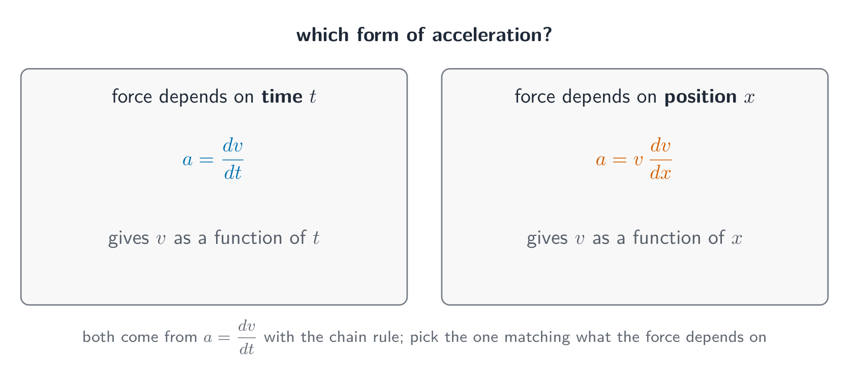
EnglishWhen the force depends on position $x$, use acceleration in the form $a = v\dfrac{dv}{dx}$, which turns Newton's law into a differential equation 微分方程 relating $v$ and $x$.
Worked example. A particle of mass $8\ \text{kg}$ moves along a line under a variable force 变力 of size $(x^3 + 4x)\ \text{N}$ acting in the direction of motion. When $x = 0$, $v = 1$. Find $v$ in terms of $x$.
Newton's law gives $8v\dfrac{dv}{dx} = x^3 + 4x$. Separating and integrating:
$$\int 8v\,dv = \int (x^3 + 4x)\,dx \;\Rightarrow\; 4v^2 = \tfrac14 x^4 + 2x^2 + C.$$At $x = 0$, $v = 1$ gives $C = 4$, so $4v^2 = \tfrac14 x^4 + 2x^2 + 4 = 4\left(\tfrac{x^2}{4} + 1\right)^2$. Hence $v = \tfrac14 x^2 + 1$.РусскийКогда сила зависит от положения $x$, используйте ускорение в виде $a = v\dfrac{dv}{dx}$, что превращает закон Ньютона в дифференциальное уравнение, связывающее $v$ и $x$.
Используйте dv/dt, когда сила зависит от времени, и vdv/dx, когда она зависит от положения*Разобранный пример. Частица массой $8\ \text{kg}$ движется вдоль прямой под действием переменной силы величиной $(x^3 + 4x)\ \text{N}$, действующей в направлении движения. При $x = 0$, $v = 1$. Найдите $v$ через $x$.
Закон Ньютона дает $8v\dfrac{dv}{dx} = x^3 + 4x$. Разделяя переменные и интегрируя:
$$\int 8v\,dv = \int (x^3 + 4x)\,dx \;\Rightarrow\; 4v^2 = \tfrac14 x^4 + 2x^2 + C.$$При $x = 0$, из выражения $v = 1$ следует $C = 4$, следовательно $4v^2 = \tfrac14 x^4 + 2x^2 + 4 = 4\left(\tfrac{x^2}{4} + 1\right)^2$. Отсюда $v = \tfrac14 x^2 + 1$.
Сила, зависящая от положения, становится дифференциальным уравнением относительно скорости и координаты Explore · ИсследоватьWork from a variable force · Работа переменной силы
W = ∫ F dx
When the force changes, the work done is the area under the force–distance graph. · Когда сила изменяется, совершенная работа равна площади под графиком зависимости силы от расстояния.
Vocabulary · Словарь Train · ТренироватьEnglish Русский variable force/ˈveərɪəbl fɔːs/ переменная сила conservation of momentum/ˌkɒnsəˈveɪʃn ɒv məʊˈmentəm/ сохранения импульса Newton's experimental law/ˈnjuːtnz ekˌsperɪˈmentl lɔː/ экспериментальный закон Ньютона coefficient of restitution/ˌkəʊɪˈfɪʃənt ɒv rɪstɪˈtjuːʃn/ коэффициент восстановления bounding parabola/ˈbaʊndɪŋ pəˈræbələ/ ограничивающая парабола lamina/ˈlæmɪnə/ пластина (ламине) coplanar forces/ˌkəʊˈpleɪnə ˈfɔːsɪz/ соплосковые силы conical pendulum/ˈkɒnɪkl ˈpendjʊləm/ конический маятник normal contact force/ˈnɔːml ˈkɒntækt fɔːs/ нормальная контактная сила oblique impact/əˈbliːk ˈɪmpækt/ косой удар 3.6
Momentum · Импульс

Syllabus · Программа
EnglishCandidates should be able to: Notes and examples recall Newton’s experimental law and the definition of the coefficient of restitution, the property $0 \leqslant e \leqslant 1$, and the meaning of the terms ‘perfectly elastic’ ($e = 1$) and ‘inelastic’ ($e = 0$) use conservation of linear momentum and/or Newton’s experimental law to solve problems that may be modelled as the direct or oblique impact of two smooth spheres, or the direct or oblique impact of a smooth sphere with a fixed surface. РусскийКандидаты должны уметь: Примечания и примеры вспомнить экспериментальный закон Ньютона и определение коэффициента восстановления, свойство $0 \leqslant e \leqslant 1$, а также значение терминов «абсолютно упругий» ($e = 1$) и «неупругий» ($e = 0$) использовать закон сохранения импульса и/или экспериментальный закон Ньютона для решения задач, которые могут быть смоделированы как прямое или косое столкновение двух гладких шаров, или прямое или косое столкновение гладкого шара с неподвижной поверхностью. Source: Cambridge International syllabus · Источник: Программа Cambridge International
EnglishIn a collision, total linear momentum is conserved — the conservation of linear momentum 动量守恒. The bounciness is measured by Newton's experimental law 牛顿实验定律, which defines the coefficient of restitution 恢复系数 $e$:
$$e = \frac{\text{speed of separation}}{\text{speed of approach}}, \qquad 0 \leqslant e \leqslant 1.$$Here $e = 1$ is perfectly elastic (no energy lost) and $e = 0$ is inelastic (the bodies stay together). In an oblique impact 斜碰撞, resolve the velocities along and perpendicular to the line of impact, applying restitution along it.Worked example. A sphere $A$ of mass $2\ \text{kg}$ moving at $5\ \text{m s}^{-1}$ hits a stationary sphere $B$ of mass $3\ \text{kg}$, with $e = 0.5$. Find the speeds afterwards.
Momentum: $2(5) = 2v_A + 3v_B$, so $2v_A + 3v_B = 10$. Restitution: $v_B - v_A = 0.5(5) = 2.5$. Solving together gives $v_A = 0.5\ \text{m s}^{-1}$ and $v_B = 3.0\ \text{m s}^{-1}$.
РусскийМаятник Ньютона демонстрирует закон сохранения импульса при столкновениях. При столкновении полный линейный импульс сохраняется — это закон сохранения линейного импульса. Упругость измеряется по экспериментальному закону Ньютона, который определяет коэффициент восстановления $e$:
$$e = \frac{\text{speed of separation}}{\text{speed of approach}}, \qquad 0 \leqslant e \leqslant 1.$$Здесь $e = 1$ — абсолютно упругое столкновение (нет потери энергии), а $e = 0$ — неупругое (тела слипаются). При нецентральном ударе разложите скорости вдоль и перпендикулярно линии удара, применяя коэффициент восстановления вдоль линии удара.
Коэффициент восстановления $e$ сравнивает скорость разлета тел со скоростью их сближения. Разобранный пример. Сфера $A$ массой $2\ \text{kg}$, движущаяся со скоростью $5\ \text{m s}^{-1}$, ударяет о неподвижную сферу $B$ массой $3\ \text{kg}$, при $e = 0.5$. Найдите скорости после удара.
Импульс: $2(5) = 2v_A + 3v_B$, значит $2v_A + 3v_B = 10$. Коэффициент восстановления: $v_B - v_A = 0.5(5) = 2.5$. Решение системы дает $v_A = 0.5\ \text{m s}^{-1}$ и $v_B = 3.0\ \text{m s}^{-1}$.
Explore · ИсследоватьA collision · Столкновение
Set each mass and speed, then collide them. Total momentum is conserved — see how the velocities come out. · Установите массу и скорость каждого объекта, затем столкните их. Общий импульс сохраняется — посмотрите, какие получаются скорости.
3.6
Exam tips · Советы для экзамена
English- For projectiles, resolve into horizontal (constant velocity) and vertical ($a = g$) motion, linked by the same time.
- For a rigid body in equilibrium, take moments about a point that removes an unknown force.
- For circular motion, use $F = mv^2/r = m\omega^2 r$ towards the centre; in a vertical circle check the minimum speed at the top.
- With a variable force, use $a = v\,\frac{dv}{dx}$ and integrate; elastic PE $= \frac{\lambda x^2}{2L}$.
Русский- Для проектильных тел разложите движение на горизонтальное (равномерное) и вертикальное ($a = g$), связанные общим временем.
- Для твердого тела в равновесии составьте уравнение моментов относительно точки, исключающей неизвестную силу.
- Для кругового движения используйте $F = mv^2/r = m\omega^2 r$ к центру; в вертикальной окружности проверьте минимальную скорость в верхней точке.
- При переменной силе используйте $a = v\,\frac{dv}{dx}$ и интегрируйте; упругая потенциальная энергия $= \frac{\lambda x^2}{2L}$.
-
4
Further Probability & Statistics · Дополнительная теория вероятностей и статистика
Watch lesson · Смотреть урокEnglishThis handout covers Topic 4: Further Probability & Statistics 进阶概率统计. It adds continuous distributions, small-sample inference, the chi-squared and non-parametric tests, and probability generating functions.
РусскийЭта методичка охватывает тему 4: Дополнительная теория вероятностей и статистика. Она включает непрерывные распределения, вывод для малых выборок, критерий хи-квадрат и непараметрические тесты, а также производящие функции вероятности.
4.1
Continuous random variables · Непрерывные случайные величины

Syllabus · Программа
EnglishCandidates should be able to: Notes and examples use a probability density function which may be defined piecewise use the general result $\text{E}(g(X)) = \int f(x)g(x) \, \mathrm{d}x$ where $f(x)$ is the probability density function of the continuous random variable $X$ and $g(X)$ is a function of $X$ understand and use the relationship between the probability density function (PDF) and the cumulative distribution function (CDF), and use either to evaluate probabilities or percentiles use cumulative distribution functions (CDFs) of related variables in simple cases. e.g. given the CDF of a variable $X$, find the CDF of a related variable $Y$, and hence its PDF, e.g. where $Y = X^3$. РусскийКандидаты должны уметь: Примечания и примеры использовать функцию плотности вероятности, которая может быть задана кусочно использовать общее следствие $\text{E}(g(X)) = \int f(x)g(x) \, \mathrm{d}x$, где $f(x)$ является функцией плотности вероятности непрерывной случайной величины $X$, а $g(X)$ — функция от $X$ понимать и использовать связь между функцией плотности вероятности (PDF) и функцией распределения (CDF), а также использовать любую из них для вычисления вероятностей или перцентилей использовать функции распределения (CDF) связанных величин в простых случаях. Например, зная CDF величины $X$, найти CDF связанной величины $Y$, а затем её PDF, например, когда $Y = X^3$. Source: Cambridge International syllabus · Источник: Программа Cambridge International
EnglishA continuous variable $X$ is described by a probability density function 概率密度函数 $f(x)$, which may be defined piecewise. The probability over a range is the area under $f$, and the mean of any function of $X$ is
$$E(g(X)) = \int g(x)\,f(x)\,dx.$$The cumulative distribution function 累积分布函数 $F(x) = P(X \leqslant x)$ is the running total: $F(x) = \displaystyle\int_{-\infty}^{x} f(t)\,dt$, and $f(x) = F'(x)$. Use $F$ to find probabilities and percentiles 百分位数 (for example, the median 中位数 solves $F(x) = 0.5$).
Worked example. A variable has $f(x) = \tfrac12 x$ for $0 \leqslant x \leqslant 2$. Find the median.
The cumulative distribution function is $F(x) = \displaystyle\int_0^x \tfrac12 t\,dt = \tfrac14 x^2$. Set $F(m) = 0.5$:
$$\tfrac14 m^2 = 0.5 \;\Rightarrow\; m^2 = 2 \;\Rightarrow\; m = \sqrt{2} = 1.41.$$The distribution of a related variable. If $Y=g(X)$, find $Y$'s distribution through its cumulative function. For $Y=X^2$: $F_Y(y)=P(X^2\leqslant y)=P(-\sqrt y\leqslant X\leqslant\sqrt y)=F_X(\sqrt y)-F_X(-\sqrt y)$, then differentiate for $f_Y=F_Y'$. When $g$ is monotonic increasing there is a shortcut, $F_Y(y)=F_X\big(g^{-1}(y)\big)$.
Worked example. With $f_X(x)=\tfrac12 x$ on $[0,2]$ (so $F_X(x)=\tfrac14 x^2$), let $Y=X^2$. For $0\leqslant y\leqslant 4$, $F_Y(y)=F_X(\sqrt y)=\tfrac14 y$, so $f_Y(y)=F_Y'(y)=\tfrac14$ – that is, $Y$ is uniform on $[0,4]$.
РусскийНепреремнная переменная $X$ описывается функцией плотности вероятности $f(x)$, которая может быть задана кусочно. Вероятность попадания в диапазон равна площади под $f$, а среднее значение любой функции от $X$ равно
$$E(g(X)) = \int g(x)\,f(x)\,dx.$$Медиана находится там, где площадь под $f(x)$ слева от нее составляет ровно $0.5$. Функция накопленного распределения $F(x) = P(X \leqslant x)$ — это накопленная сумма: $F(x) = \displaystyle\int_{-\infty}^{x} f(t)\,dt$, и $f(x) = F'(x)$. Используйте $F$ для нахождения вероятностей и перцентилей (например, медиана определяет $F(x) = 0.5$).

График накопленного распределения $F(x)$ возрастает от $0$ до $1$; высота $0.5$ достигается в точке медианы. Разбор примера. Случайная величина имеет $f(x) = \tfrac12 x$ при $0 \leqslant x \leqslant 2$. Найдите медиану.
Функция накопленного распределения равна $F(x) = \displaystyle\int_0^x \tfrac12 t\,dt = \tfrac14 x^2$. Приравняйте $F(m) = 0.5$:
$$\tfrac14 m^2 = 0.5 \;\Rightarrow\; m^2 = 2 \;\Rightarrow\; m = \sqrt{2} = 1.41.$$Распределение связанной переменной. Если $Y=g(X)$, найдите распределение $Y$ через его функцию накопления. Для $Y=X^2$: $F_Y(y)=P(X^2\leqslant y)=P(-\sqrt y\leqslant X\leqslant\sqrt y)=F_X(\sqrt y)-F_X(-\sqrt y)$, затем дифференцируйте для получения $f_Y=F_Y'$. Когда $g$ монотонно возрастает, существует упрощение, $F_Y(y)=F_X\big(g^{-1}(y)\big)$.
Разбор примера. Имеется $f_X(x)=\tfrac12 x$ на интервале $[0,2]$ (поэтому $F_X(x)=\tfrac14 x^2$), пусть $Y=X^2$. Для $0\leqslant y\leqslant 4$, $F_Y(y)=F_X(\sqrt y)=\tfrac14 y$, следовательно $f_Y(y)=F_Y'(y)=\tfrac14$ — то есть $Y$ распределена равномерно на $[0,4]$.
Explore · ИсследоватьContinuous random variables · Непрерывные случайные величины
P(a < X < b) = ∫ f(x) dx
For a continuous variable, probability is the area under the density curve. · Для непрерывной переменной вероятность равна площади под кривой плотности.
Vocabulary · Словарь Train · ТренироватьEnglish Русский probability density function/ˌprɒbəˈbɪlɪti ˈdensɪti ˈfʌŋkʃn/ функция плотности вероятности cumulative distribution function/ˈkjuːmjʊlətɪv ˌdɪstrɪˈbjuːʃn ˈfʌŋkʃn/ функция распределения percentiles/pəˈsentaɪlz/ перцентилей median/ˈmiːdiːən/ медианой hypothesis test/haɪˈpɒθəsɪs test/ статистическая гипотеза confidence interval/ˈkɒnfɪdəns ˈɪntəvl/ доверительный интервал pooled estimate/puːld ˈestɪmət/ объединенная оценка chi-squared test/kaɪ skweəd test/ критерий хи-квадрат theoretical distribution/θɪəˈretɪkl ˌdɪstrɪˈbjuːʃn/ теоретическое распределение degrees of freedom/dɪˈɡriːz ɒv ˈfriːdəm/ число степеней свободы goodness of fit/ˈɡʊdnəs ɒv fɪt/ соответствия independence/ˌɪndɪˈpendəns/ независимости contingency table/kənˈtɪndʒənsi ˈteɪbl/ таблица сопряженности non-parametric test/nɒn ˌpærəˈmetrɪk test/ непараметрический тест 4.2
Inference using normal and t-distributions · Вывод на основе нормального и t-распределений

Syllabus · Программа
EnglishCandidates should be able to: Notes and examples formulate hypotheses and apply a hypothesis test concerning the population mean using a small sample drawn from a normal population of unknown variance, using a t-test calculate a pooled estimate of a population variance from two samples Calculations based on either raw or summarised data may be required. formulate hypotheses concerning the difference of population means, and apply, as appropriate: - a 2-sample t-test - a paired sample t-test - a test using a normal distribution The ability to select the test appropriate to the circumstances of a problem is expected. determine a confidence interval for a population mean, based on a small sample from a normal population with unknown variance, using a t-distribution determine a confidence interval for a difference of population means, using a t-distribution or a normal distribution, as appropriate. РусскийКандидаты должны уметь: Примечания и примеры формулировать гипотезы и применять проверку гипотезы относительно среднего значения генеральной совокупности на основе малой выборки, выбранной из нормального распределения с неизвестной дисперсией, используя t-критерий вычислять объединенную оценку дисперсии генеральной совокупности по двум выборкам Могут потребоваться расчеты как на основе исходных данных, так и на основе сводных данных. Формулировать гипотезы относительно разности средних генеральных совокупностей и применять, где уместно: - t-критерий для выборки ⟨2⟩ - ** paired t-критерий (для парных выборок)** - тест с использованием нормального распределения Ожидается способность выбирать тест, соответствующий обстоятельствам задачи. определить доверительный интервал для среднего значения генеральной совокупности на основе малой выборки из нормального распределения с неизвестной дисперсией, используя t-распределение определить доверительный интервал для разности средних значений генеральных совокупностей, используя t-распределение или нормальное распределение, в зависимости от обстоятельств. Source: Cambridge International syllabus · Источник: Программа Cambridge International
EnglishWhen a sample is small and the population variance is unknown, base your hypothesis test 假设检验 on the $t$-distribution instead of the normal. The same idea gives a confidence interval 置信区间 for the mean:
$$\bar{x} \pm t\,\frac{s}{\sqrt{n}},$$where $t$ comes from the $t$-tables with $n - 1$ degrees of freedom. To compare two populations, use a two-sample (2-sample) or paired-sample $t$-test, after finding a pooled estimate 合并估计 of the shared variance when appropriate.Worked example. A sample of $n = 10$ has mean $\bar{x} = 50$ and standard deviation $s = 4$. Find a $95\%$ confidence interval for the mean (use $t = 2.262$ for $9$ degrees of freedom).
$$50 \pm 2.262\times\frac{4}{\sqrt{10}} = 50 \pm 2.86 \;\Rightarrow\; (47.1,\ 52.9).$$РусскийДоска Гальтона: падающие шары через штырьки складываются в колоколообразное нормальное распределение. Когда выборка мала, а дисперсия генеральной совокупности неизвестна, основывайте гипотезу на распределении $t$ вместо нормального. Та же идея дает доверительный интервал для среднего:
$$\bar{x} \pm t\,\frac{s}{\sqrt{n}},$$где $t$ берется из таблиц распределения $t$ с $n - 1$ степенями свободы. Для сравнения двух совокупностей используйте двухвыборочный (2-выборочный) или парный тест $t$, предварительно найдя объединенную оценку общей дисперсии при необходимости.
Для малой выборки распределение $t$ более полого с тяжелыми хвостами, поэтому его критические значения больше. Разобранное решение. Образец $n = 10$ имеет среднее значение $\bar{x} = 50$ и стандартное отклонение $s = 4$. Найдите доверительный интервал для среднего со степенью достоверности $95\%$ (используйте $t = 2.262$ для $9$ степеней свободы).
$$50 \pm 2.262\times\frac{4}{\sqrt{10}} = 50 \pm 2.86 \;\Rightarrow\; (47.1,\ 52.9).$$Explore · ИсследоватьWhy small samples need t instead of z · Почему малым выборкам нужен t вместо z
With $\sigma$ unknown you use $t$, and $t$ has heavier tails than the normal (drawn dashed behind it) — so its critical values are larger and the interval is wider. At the worked example's $9$ degrees of freedom the widget reads $t^* = 2.262$, exactly the table value used above. Sweep df up and $t$ collapses onto the normal. · При неизвестном $\sigma$ используется $t$, и $t$ имеет более тяжелые хвосты, чем нормальное (нарисовано пунктиром позади него) — поэтому его критические значения больше, а интервал шире. При $9$ степенях свободы, указанных в разобранном решении, виджет показывает $t^* = 2.262$, точно такое же табличное значение, что использовалось выше. Прокрутите df вверх, и $t$ совпадет с нормальным распределением.
Explore · ИсследоватьThe normal distribution · Нормальное распределение
Shade a tail to find a probability — the basis of confidence intervals and hypothesis tests. · Заштрихуйте хвост, чтобы найти вероятность — это основа доверительных интервалов и тестов гипотез.
4.3
Chi-squared tests · Критерии хи-квадрат
Syllabus · Программа
EnglishCandidates should be able to: Notes and examples fit a theoretical distribution, as prescribed by a given hypothesis, to given data Questions will not involve lengthy calculations. use a $\chi^2$-test, with the appropriate number of degrees of freedom, to carry out the corresponding goodness of fit analysis Classes should be combined so that each expected frequency is at least 5. use a $\chi^2$-test, with the appropriate number of degrees of freedom, for independence in a contingency table. Yates’ correction is not required. Where appropriate, either rows or columns should be combined so that the expected frequency in each cell is at least 5. РусскийКандидаты должны уметь: Примечания и примеры подбирать теоретическое распределение, предписанное данной гипотезой, к имеющимся данным Задания не будут включать длительные вычисления. использовать $\chi^2$-критерий с соответствующим числом степеней свободы для проведения анализа соответствия (goodness of fit) Классы следует объединять так, чтобы каждая ожидаемая частота была не менее 5. использовать $\chi^2$-критерий с соответствующим числом степеней свободы для проверки независимости в таблице сопряженности. Поправка Йейтса не требуется. При необходимости следует объединять строки или столбцы так, чтобы ожидаемая частота в каждой ячейке составляла не менее 5. Source: Cambridge International syllabus · Источник: Программа Cambridge International
EnglishA $\chi^2$-test (chi-squared test 卡方检验) compares observed counts $O$ with expected counts $E$ from a theoretical distribution 理论分布:
$$\chi^2 = \sum \frac{(O - E)^2}{E}.$$Compare this with a table value for the right number of degrees of freedom 自由度. Two uses: a goodness of fit 拟合优度 test (does the data follow the proposed model?), and a test for independence 独立性 of two variables in a contingency table 列联表.Worked example. Four equally likely categories give observed counts $20, 30, 25, 25$ (so each expected count is $25$). Test the fit at the $5\%$ level.
$$\chi^2 = \frac{(20-25)^2 + (30-25)^2 + 0 + 0}{25} = \frac{25 + 25}{25} = 2.$$With $4 - 1 = 3$ degrees of freedom the table value is $7.815$. Since $2 < 7.815$, do not reject the model.РусскийКритерий $\chi^2$ (χ²-критерий) сравнивает наблюдаемые частоты $O$ с ожидаемыми частотами $E$ из теоретического распределения:
$$\chi^2 = \sum \frac{(O - E)^2}{E}.$$Сравните это значение с табличным для соответствующего числа степеней свободы. Два применения: тест пригодности (соответствуют ли данные предложенной модели?) и тест на независимость двух переменных в таблице сопряженности.Критерий отвергает модель, когда $\chi^2$ превышает критическое значение, попадая в заштрихованный правый хвост $5\%$. Разбор примера. Четыре равновероятные категории дают наблюдаемые частоты $20, 30, 25, 25$ (поэтому каждая ожидаемая частота равна $25$). Проверьте соответствие на уровне значимости $5\%$.
$$\chi^2 = \frac{(20-25)^2 + (30-25)^2 + 0 + 0}{25} = \frac{25 + 25}{25} = 2.$$При $4 - 1 = 3$ степенях свободы табличное значение равно $7.815$. Поскольку $2 < 7.815$, не отвергаем модель.Explore · ИсследоватьThe chi-squared distribution and its 5% tail · Распределение хи-квадрат и его хвост на 5%
The worked example on this page gives $\chi^2 = 2$ with $3$ degrees of freedom against a table value of $7.815$ — the widget reproduces both. Drag df to see why the critical value changes with the number of categories. · Разобранное решение на этой странице дает $\chi^2 = 2$ при $3$ степенях свободы против табличного значения $7.815$ — виджет воспроизводит оба. Перетащите df, чтобы увидеть, почему критическое значение меняется в зависимости от числа категорий.
Explore · ИсследоватьChi-squared test route · Маршрут хи-квадрат теста
Follow observed and expected counts to a test decision. · Следуйте наблюдаемым и ожидаемым частотам для принятия решения по тесту.
4.4
Non-parametric tests · Непараметрические тесты

Syllabus · Программа
EnglishCandidates should be able to: Notes and examples understand the idea of a non-parametric test and appreciate situations in which such a test might be useful e.g. when sampling from a population which cannot be assumed to be normally distributed. understand the basis of the sign test, the Wilcoxon signed-rank test and the Wilcoxon rank-sum test Including knowledge that Wilcoxon tests are valid only for symmetrical distributions. use a single-sample sign test and a single-sample Wilcoxon signed-rank test to test a hypothesis concerning a population median Including the use of normal approximations where appropriate. Questions will not involve tied ranks or observations equal to the population median value being tested. use a paired-sample sign test, a Wilcoxon matched-pairs signed-rank test and a Wilcoxon rank-sum test, as appropriate, to test for identity of populations. Including the use of normal approximations where appropriate. Questions will not involve tied ranks or zero‑difference pairs. РусскийКандидаты должны уметь: Примечания и примеры понимать концепцию непараметрического критерия и оценивать ситуации, в которых такой критерий может быть полезен например, при выборочном исследовании из генеральной совокупности, которую нельзя считать нормально распределенной. понимать основу знакового теста, теста Вилкоксона о рангах со знаками и теста Вилкоксона о сумме рангов Включая знание того, что тесты Вилкоксона применимы только для симметричных распределений. использовать одновыборочный знаковый тест и одновыборочный тест Вилкоксона о рангах со знаками для проверки гипотезы относительно медианы генеральной совокупности Включая использование нормальных приближений там, где это уместно. Задания не будут включать одинаковые ранги или наблюдения, равные проверяемому значению медианы генеральной совокупности. использовать парный знаковый тест, тест Вилкоксона для спаренных выборок о рангах со знаками и тест Вилкоксона о сумме рангов (при необходимости) для проверки равенства генеральных совокупностей. Включая использование нормальных приближений там, где это уместно. Задания не будут включать одинаковые ранги или пары нулевой разницы. Source: Cambridge International syllabus · Источник: Программа Cambridge International
EnglishA non-parametric test 非参数检验 makes no assumption that the data is normal, so it is useful when that assumption fails. The basic ones are:
- the sign test 符号检验: count how many values fall above and below a proposed median, and test those counts with a binomial model;
- the Wilcoxon signed-rank test 威尔科克森符号秩检验 (the matched-pairs test for paired data), which also uses the sizes of the differences, not just their signs;
- the Wilcoxon rank-sum test 威尔科克森秩和检验, for comparing two separate samples.
Worked example. Test whether a median is $5$. In a sample of $10$ values (none equal to $5$), $9$ lie above $5$ and $1$ lies below. Test at the $5\%$ level (two-tailed).
Under $H_0$ (median $= 5$) the number above follows $B(10, 0.5)$. The observed result ($9$ above) is extreme, so find $P(X \geq 9) = \binom{10}{9}(0.5)^{10} + (0.5)^{10} = \dfrac{11}{1024} = 0.0107$. For a two-tailed test compare with $\tfrac{1}{2}(5\%) = 0.025$. Since $0.0107 < 0.025$, reject $H_0$: there is evidence the median is not $5$.
РусскийНепараметрический тест не предполагает нормальное распределение данных, поэтому он полезен, когда это предположение нарушается. Основные из них:
- знаковый тест: подсчитайте, сколько значений находятся выше и ниже предполагаемой медианы, и протестируйте эти подсчеты с помощью биномиальной модели;
- критерий Вилкоксона для связанных выборок (тест для парных данных), который также использует величины различий, а не только их знаки;
- критерий Вилкоксона для независимых выборок, для сравнения двух отдельных выборок.
Знаковый тест подсчитывает, сколько значений находится выше и ниже предлагаемой медианы, затем проверяет эти подсчеты с помощью биномиальной модели Разобранный пример. Проверьте, является ли медиана равной $5$. В выборке из $10$ значений (ни одно не равно $5$), $9$ находятся выше $5$, а $1$ — ниже. Проведите тест на уровне значимости $5\%$ (двусторонний).
При условии $H_0$ (медиана $= 5$) количество наблюдений выше нее следует распределению $B(10, 0.5)$. Наблюдаемый результат ($9$ над медианой) является экстремальным, поэтому найдите P-значение $P(X \geq 9) = \binom{10}{9}(0.5)^{10} + (0.5)^{10} = \dfrac{11}{1024} = 0.0107$. Для двустороннего теста сравните со значением $\tfrac{1}{2}(5\%) = 0.025$. Поскольку $0.0107 < 0.025$, отвергаем гипотезу $H_0$: есть доказательства того, что медиана не равна $5$.
Explore · ИсследоватьNon-parametric test chooser · Выбор непараметрического теста
Choose the rank-based test that matches the data situation. · Выберите ранговый тест, соответствующий ситуации с данными.
Vocabulary · Словарь Train · ТренироватьEnglish Русский sign test/saɪn test/ тест знаков Wilcoxon signed-rank test/ˈwɪlkɒksn saɪnd ræŋk test/ критерий Вилкоксона для связанных выборок Wilcoxon rank-sum test/ˈwɪlkɒksn ræŋk sʌm test/ критерий Вилкоксона probability generating function/ˌprɒbəˈbɪlɪti ˈdʒenəreɪtɪŋ ˈfʌŋkʃn/ функция порождения вероятностей Further Probability & Statistics/ˈfɜːðə ˌprɒbəˈbɪlɪti ænd stəˈtɪstɪks/ Дополнительная теория вероятностей и статистика 4.5
Probability generating functions · Генерирующие функции вероятностей

Syllabus · Программа
EnglishCandidates should be able to: Notes and examples understand the concept of a probability generating function (PGF) and construct and use the PGF for given distributions Including the discrete uniform, binomial, geometric and Poisson distributions. use formulae for the mean and variance of a discrete random variable in terms of its PGF, and use these formulae to calculate the mean and variance of a given probability distribution use the result that the PGF of the sum of independent random variables is the product of the PGFs of those random variables. РусскийКандидаты должны уметь: Примечания и примеры понимать концепцию функции порождения вероятностей (PGF) и составлять и использовать PGF для заданных распределений Включая дискретное равномерное, биномиальное, геометрическое и пуассоновское распределения. использовать формулы для математического ожидания и дисперсии дискретной случайной переменной через её PGF, а также применять эти формулы для вычисления математического ожидания и дисперсии заданного распределения вероятностей использовать результат о том, что PGF суммы независимых случайных величин является произведением их PGF. Source: Cambridge International syllabus · Источник: Программа Cambridge International
EnglishThe probability generating function 概率母函数 of a discrete variable $X$ is
$$G(t) = E(t^X) = \sum_x P(X = x)\,t^x.$$It packs the whole distribution into one function. The mean and variance come from its derivatives at $t = 1$: $E(X) = G'(1)$ and $\mathrm{Var}(X) = G''(1) + G'(1) - \big(G'(1)\big)^2$. Also, the PGF of a sum of independent variables is the product of their PGFs.Worked example. $X$ has $P(X=0) = 0.5$, $P(X=1) = 0.3$, $P(X=2) = 0.2$. Find $E(X)$ using the PGF.
Here $G(t) = 0.5 + 0.3t + 0.2t^2$, so $G'(t) = 0.3 + 0.4t$ and
$$E(X) = G'(1) = 0.3 + 0.4 = 0.7.$$РусскийИгральные кости: отправная точка для теории вероятностей и дискретных случайных величин. Генерирующая функция вероятностей дискретной случайной величины $X$ имеет вид
$$G(t) = E(t^X) = \sum_x P(X = x)\,t^x.$$Она упаковывает всё распределение в одну функцию. Математическое ожидание и дисперсия получаются из её производных при $t = 1$: $E(X) = G'(1)$ и $\mathrm{Var}(X) = G''(1) + G'(1) - \big(G'(1)\big)^2$. Кроме того, ГФ суммы независимых величин равна произведению их ГФ.Разбор примера. Случайная величина $X$ принимает значения $P(X=0) = 0.5$, $P(X=1) = 0.3$, $P(X=2) = 0.2$. Найдите P-функцию (PGF) $E(X)$.
Здесь $G(t) = 0.5 + 0.3t + 0.2t^2$, следовательно $G'(t) = 0.3 + 0.4t$ и
$$E(X) = G'(1) = 0.3 + 0.4 = 0.7.$$
ГФ честной игральной кости упаковывает одинаковые массы от 1 до 6 в G(t) Explore · ИсследоватьProbability generating function lab · Лабораторная работа: функция порождения вероятностей
G(x) = p0 + p1 x + p2 x^2 + ...
Change x and see how a PGF stores probabilities in powers of x. · Измените x и посмотрите, как ФПВ хранит вероятности в степенях x.
4.5
Exam tips · Советы для экзамена
English- For a continuous random variable, the pdf integrates to $1$ over its range, and $E(X) = \int x f(x)\,dx$.
- Use the $t$-distribution when the sample is small and the population variance is unknown; state the degrees of freedom.
- For a chi-squared test compute $\sum (O-E)^2/E$, compare with the critical value at the right degrees of freedom, and combine classes with $E < 5$.
- State $H_0$ and $H_1$ and give the conclusion in context for every test.
Русский- Для непрерывной случайной величины плотность вероятности интегрируется до $1$ по всему диапазону, а интеграл равен $E(X) = \int x f(x)\,dx$.
- Используйте распределение t-Стьюдента ($t$-распределение), когда выборка мала, а генеральная дисперсия неизвестна; укажите число степеней свободы.
- Для χ²-критерия вычислите статистику $\sum (O-E)^2/E$, сравните её с критическим значением для соответствующих степеней свободы и объедините классы с малыми частотами $E < 5$.
- Укажите нулевую и альтернативную гипотезы $H_0$ и $H_1$ и дайте вывод в контексте задачи для каждого теста.