Funções Exponenciais e Logarítmicas

Pré-Cálculo do AP · Topic 2 · ⁨Tópico 2⁩

Train · ⁨Treinar⁩

Video lesson for this topic · ⁨Videoaula para este tópico⁩ Open the video page · ⁨Abrir a página do vídeo⁩

2.1

Change in Arithmetic and Geometric Sequences · ⁨Mudança em Sequências Aritméticas e Geométricas⁩

Syllabus · ⁨Programa⁩

English

Learning Objective 2.1.A: Express arithmetic sequences found in mathematical and contextual scenarios as functions of the whole numbers.

2.1.A.1 A sequence is a function from the whole numbers to the real numbers. Consequently, the graph of a sequence consists of discrete points instead of a curve.
2.1.A.2 Successive terms in an arithmetic sequence have a common difference, or constant rate of change.
2.1.A.3 The general term of an arithmetic sequence with a common difference $d$ is denoted by $a_n$ and is given by $a_n = a_0 + dn$, where $a_0$ is the initial value, or by $a_n = a_k + d(n - k)$, where $a_k$ is the $k$th term of the sequence.

Learning Objective 2.1.B: Express geometric sequences found in mathematical and contextual scenarios as functions of the whole numbers.

2.1.B.1 Successive terms in a geometric sequence have a common ratio, or constant proportional change.
2.1.B.2 The general term of a geometric sequence with a common ratio $r$ is denoted by $g_n$ and is given by $g_n = g_0 r^n$, where $g_0$ is the initial value, or by $g_n = g_k r^{(n-k)}$, where $g_k$ is the $k$th term of the sequence.
2.1.B.3 Increasing arithmetic sequences increase equally with each step, whereas increasing geometric sequences increase by a larger amount with each successive step.

Português

Objetivo de Aprendizagem 2.1.A: Expressar sequências aritméticas encontradas em cenários matemáticos e contextuais como funções dos números inteiros.

2.1.A.1 Uma sequência é uma função dos números inteiros para os números reais. Consequentemente, o gráfico de uma sequência consiste em pontos discretos em vez de uma curva.
2.1.A.2 Termos sucessivos em uma sequência aritmética têm uma diferença comum, ou taxa de variação constante.
2.1.A.3 O termo geral de uma sequência aritmética com diferença comum $d$ é denotado por $a_n$ e é dado por $a_n = a_0 + dn$, onde $a_0$ é o valor inicial, ou por $a_n = a_k + d(n - k)$, onde $a_k$ é o ⟨$k$⟩-ésimo termo da sequência.

Objetivo de Aprendizagem 2.1.B: Expressar sequências geométricas encontradas em cenários matemáticos e contextuais como funções dos números inteiros.

2.1.B.1 Termos sucessivos em uma sequência geométrica têm uma razão comum, ou mudança proporcional constante.
2.1.B.2 O termo geral de uma sequência geométrica com razão comum $r$ é denotado por $g_n$ e é dado por $g_n = g_0 r^n$, onde $g_0$ é o valor inicial, ou por $g_n = g_k r^{(n-k)}$, onde $g_k$ é o ⟨$k$⟩-ésimo termo da sequência.
2.1.B.3 Sequências aritméticas crescentes aumentam igualmente a cada passo, enquanto sequências geométricas crescentes aumentam em uma quantidade maior a cada passo sucessivo.

Source: College Board AP Course and Exam Description · ⁨Fonte: College Board AP Course and Exam Description⁩

English

Geometric series & convergence

A sequence 数列 is a function from the whole numbers to the real numbers, so its graph is discrete points, not a curve.

An arithmetic sequence 等差数列 has a common difference 公差 $d$ (a constant rate of change): $a_n = a_0 + dn$, or from a known term, $a_n = a_k + d(n-k)$.
A geometric sequence 等比数列 has a common ratio 公比 $r$ (a constant proportional change): $g_n = g_0\,r^{\,n}$, or $g_n = g_k\,r^{\,(n-k)}$.

An increasing arithmetic sequence grows by the same amount each step; an increasing geometric sequence grows by a larger amount each step.

Worked example. An arithmetic sequence with $a_0=3$ and $d=5$ has $a_4=3+5(4)=23$. A geometric sequence with $g_0=2$ and $r=3$ has $g_4=2\cdot3^4=162$ – addition versus multiplication makes the geometric one pull far ahead.

Português

Série geométrica & convergência

Uma sequência 数列 é uma função dos números inteiros para os números reais, portanto seu gráfico são pontos discretos, não uma curva.

Uma sequência aritmética sobe em passos iguais; uma geométrica multiplica por uma razão

Uma sequência aritmética 等差数列 tem uma diferença comum 公差 $d$ (uma taxa de mudança constante): $a_n = a_0 + dn$, ou a partir de um termo conhecido, $a_n = a_k + d(n-k)$.
Uma sequência geométrica 等比数列 tem uma razão comum 公比 $r$ (uma mudança proporcional constante): $g_n = g_0\,r^{\,n}$, ou $g_n = g_k\,r^{\,(n-k)}$.

Uma sequência aritmética crescente cresce na mesma quantidade a cada passo; uma sequência geométrica crescente cresce em uma quantidade maior a cada passo.

Exemplo resolvido. Uma sequência aritmética com $a_0=3$ e $d=5$ tem $a_4=3+5(4)=23$. Uma sequência geométrica com $g_0=2$ e $r=3$ tem $g_4=2\cdot3^4=162$ – a adição versus a multiplicação faz a geométrica ultrapassar muito.

Explore · ⁨Explorar⁩

Compare o crescimento aritmético e geométrico

Uma sequência aritmética adiciona um passo fixo a cada termo (linear); uma sequência geométrica multiplica por uma razão fixa (exponencial). Mude a razão e observe os termos explodirem ou decaírem.

2.2

Change in Linear and Exponential Functions · ⁨Mudança em Funções Lineares e Exponenciais⁩

Syllabus · ⁨Programa⁩

English

Learning Objective 2.2.A: Construct functions of the real numbers that are comparable to arithmetic and geometric sequences.

2.2.A.1 Linear functions of the form $f(x) = b + mx$ are similar to arithmetic sequences of the form $a_n = a_0 + dn$, as both can be expressed as an initial value ($b$ or $a_0$) plus repeated addition of a constant rate of change, the slope ($m$ or $d$).
2.2.A.2 Similar to arithmetic sequences of the form $a_n = a_k + d(n - k)$, which are based on a known difference, $d$, and a $k$th term, linear functions can be expressed in the form $f(x) = y_i + m(x - x_i)$ based on a known slope, $m$, and a point, $(x_i, y_i)$.
2.2.A.3 Exponential functions of the form $f(x) = ab^x$ are similar to geometric sequences of the form $g_n = g_0 r^n$, as both can be expressed as an initial value ($a$ or $g_0$) times repeated multiplication by a constant proportion ($b$ or $r$).
2.2.A.4 Similar to geometric sequences of the form $g_n = g_k r^{(n-k)}$, which are based on a known ratio, $r$, and a $k$th term, exponential functions can be expressed in the form $f(x) = y_i r^{(x - x_i)}$ based on a known ratio, $r$, and a point, $(x_i, y_i)$.
2.2.A.5 Sequences and their corresponding functions may have different domains.

Português

Objetivo de Aprendizagem 2.2.A: Construir funções dos números reais que sejam comparáveis a sequências aritméticas e geométricas.

2.2.A.1 Funções lineares da forma $f(x) = b + mx$ são semelhantes a sequências aritméticas da forma $a_n = a_0 + dn$, pois ambas podem ser expressas como um valor inicial ($b$ ou $a_0$) mais a adição repetida de uma taxa de variação constante, a inclinação ($m$ ou $d$).
2.2.A.2 Semelhante às sequências aritméticas da forma $a_n = a_k + d(n - k)$, que se baseiam em uma diferença conhecida, $d$, e em um termo de ordem $k$, as funções lineares podem ser expressas na forma $f(x) = y_i + m(x - x_i)$ com base em uma inclinação conhecida, $m$, e em um ponto, $(x_i, y_i)$.
2.2.A.3 Funções exponenciais da forma $f(x) = ab^x$ são semelhantes a sequências geométricas da forma $g_n = g_0 r^n$, pois ambas podem ser expressas como um valor inicial ($a$ ou $g_0$) vezes a multiplicação repetida por uma proporção constante ($b$ ou $r$).
2.2.A.4 Semelhante às sequências geométricas da forma $g_n = g_k r^{(n-k)}$, que se baseiam em uma razão conhecida, $r$, e em um termo de ordem $k$, as funções exponenciais podem ser expressas na forma $f(x) = y_i r^{(x - x_i)}$ com base em uma razão conhecida, $r$, e em um ponto, $(x_i, y_i)$.
2.2.A.5 Sequências e suas funções correspondentes podem ter domínios diferentes.

Source: College Board AP Course and Exam Description · ⁨Fonte: College Board AP Course and Exam Description⁩

English

Sequences have continuous cousins:

Linear functions $f(x)=b+mx$ mirror arithmetic sequences – an initial value plus repeated addition of the slope $m$. Point form: $f(x)=y_i+m(x-x_i)$.
Exponential functions $f(x)=ab^x$ mirror geometric sequences – an initial value times repeated multiplication by the base $b$. Point form: $f(x)=y_i\,r^{\,(x-x_i)}$.

The difference: linear = repeated addition, exponential = repeated multiplication. (A sequence and its function may have different domains.)

Português

Um corredor: modelos exponenciais e logarítmicos capturam taxas de crescimento e decaimento em contexto

Sequências têm primos contínuos:

Funções lineares $f(x)=b+mx$ espelham sequências aritméticas – um valor inicial mais adições repetidas da inclinação $m$. Forma pontual: $f(x)=y_i+m(x-x_i)$.
Funções exponenciais $f(x)=ab^x$ espelham sequências geométricas – um valor inicial multiplicado por multiplicações repetidas pela base $b$. Forma pontual: $f(x)=y_i\,r^{\,(x-x_i)}$.

A diferença: linear = adição repetida, exponencial = multiplicação repetida. (Uma sequência e sua função podem ter domínios diferentes.)

2.3

Exponential Functions · ⁨Funções Exponenciais⁩

Syllabus · ⁨Programa⁩

English

Learning Objective 2.3.A: Identify key characteristics of exponential functions.

2.3.A.1 The general form of an exponential function is $f(x) = ab^x$, with the initial value $a$, where $a \neq 0$, and the base $b$, where $b > 0$, and $b \neq 1$. When $a > 0$ and $b > 1$, the exponential function is said to demonstrate exponential growth. When $a > 0$ and $0 < b < 1$, the exponential function is said to demonstrate exponential decay.
2.3.A.2 When the natural numbers are input values in an exponential function, the input value specifies the number of factors of the base to be applied to the function's initial value. The domain of an exponential function is all real numbers.
2.3.A.3 Because the output values of exponential functions in general form are proportional over equal-length input-value intervals, exponential functions are always increasing or always decreasing, and their graphs are always concave up or always concave down. Consequently, exponential functions do not have extrema except on a closed interval, and their graphs do not have points of inflection.
2.3.A.4 If the values of the additive transformation function $g(x) = f(x) + k$ of any function $f$ are proportional over equal-length input-value intervals, then $f$ is exponential.

Português

Objetivo de Aprendizagem 2.3.A: Identificar características-chave das funções exponenciais.

2.3.A.1 A forma geral de uma função exponencial é $f(x) = ab^x$, com o valor inicial $a$, onde $a \neq 0$, e a base $b$, onde $b > 0$, e $b \neq 1$. Quando $a > 0$ e $b > 1$, diz-se que a função exponencial demonstra crescimento exponencial. Quando $a > 0$ e $0 < b < 1$, diz-se que a função exponencial demonstra decadência exponencial.
2.3.A.2 Quando os números naturais são valores de entrada em uma função exponencial, o valor de entrada especifica o número de fatores da base a serem aplicados ao valor inicial da função. O domínio de uma função exponencial é todos os números reais.
2.3.A.3 Como os valores de saída das funções exponenciais na forma geral são proporcionais em intervalos de valor de entrada de comprimento igual, as funções exponenciais estão sempre aumentando ou sempre diminuindo, e seus gráficos são sempre côncavos para cima ou sempre côncavos para baixo. Consequentemente, as funções exponenciais não têm extremos exceto em um intervalo fechado, e seus gráficos não têm pontos de inflexão.
2.3.A.4 Se os valores da função de transformação aditiva $g(x) = f(x) + k$ de qualquer função $f$ forem proporcionais em intervalos de valor de entrada de comprimento igual, então $f$ é exponencial.

Source: College Board AP Course and Exam Description · ⁨Fonte: College Board AP Course and Exam Description⁩

English

The general exponential function 指数函数 is $f(x)=ab^x$ with initial value 初始值 $a\neq 0$ and base 底数 $b>0,\ b\neq 1$. Domain: all real numbers.

$a>0,\ b>1$ gives exponential growth 指数增长; $a>0,\ 0 gives exponential decay 指数衰减.
Outputs are proportional over equal-length input intervals. So an exponential is always increasing or always decreasing, and always concave up or always concave down – it has no extrema (except on a closed interval) and no points of inflection.

Português

A função exponencial geral 指数函数 é $f(x)=ab^x$ com valor inicial 初始值 $a\neq 0$ e base 底数 $b>0,\ b\neq 1$. Domínio: todos os números reais.

Decaimento exponencial: uma porcentagem fixa é perdida a cada período

$a>0,\ b>1$ dá crescimento exponencial 指数增长; $a>0,\ 0 dá decaimento exponencial 指数衰减.
As saídas são proporcionais em intervalos de entrada de comprimento igual. Portanto, uma exponencial é sempre crescente ou sempre decrescente, e sempre côncava para cima ou sempre côncava para baixo – ela não possui extremos (exceto em um intervalo fechado) nem pontos de inflexão.

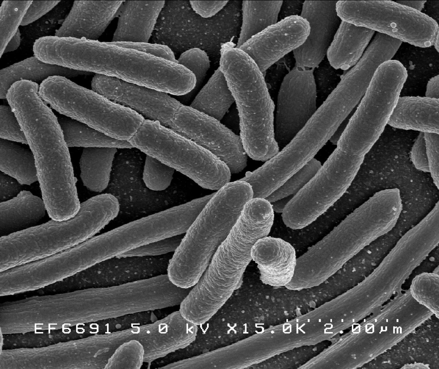
Bactérias sob microscópio: modelos exponenciais descrevem populações que crescem por um fator constante a cada etapa temporal

Explore · ⁨Explorar⁩

Explore uma curva exponencial

y = a·e^(bx) + c

Uma função exponencial muda por um fator constante em etapas iguais, então ela cresce (ou decai) cada vez mais rápido. A constante $c$ define a assíntota horizontal que ela abraça.

Vocabulary · ⁨Vocabulário⁩ Train · ⁨Treinar⁩

English · ⁨Inglês⁩	Chinese · ⁨Chinês⁩	Pinyin
sequence/ˈsiːkwəns/	数列	shù liè
arithmetic sequence/əˈrɪθmətɪk ˈsiːkwəns/	等差数列	děng chā shù liè
common difference/ˈkɒmən ˈdɪfrəns/	公差	gōng chāi
geometric sequence/ˌdʒiːəʊˈmetrɪk ˈsiːkwəns/	等比数列	děng bǐ shù liè
common ratio/ˈkɒmən ˈreɪʃɪəʊ/	公比	gōng bǐ
exponential function/ˌekspəˈnenʃl ˈfʌŋkʃn/	指数函数	zhǐ shù hán shù
initial value/ɪˈnɪʃl ˈvæljuː/	初始值	chū shǐ zhí
base/beɪs/	底数	dǐ shù
exponential growth/ˌekspəˈnenʃl ɡrəʊθ/	指数增长	zhǐ shù zēng zhǎng
exponential decay/ˌekspəˈnenʃl dɪˈkeɪ/	指数衰减	zhǐ shù shuāi jiǎn
root/ruːt/	方根	fāng gēn
exponential regression/ˌekspəˈnenʃl rɪˈɡreʃn/	指数回归	zhǐ shù huí guī
natural base/ˈnætʃərəl beɪs/	自然底数	zì rán dǐ shù
residual plot/rɪˈsɪdʒuːəl plɒt/	残差图	cán chà tú
residual/rɪˈsɪdʒuːəl/	残差	cán chà
composite function/ˈkɒmpəzɪt ˈfʌŋkʃn/	复合函数	fù hé hán shù
identity function/aɪˈdentɪti ˈfʌŋkʃn/	恒等函数	héng děng hán shù
invertible/ɪnˈvɜːtɪbl/	可逆	kě nì

2.4

Exponential Function Manipulation · ⁨Manipulação da Função Exponencial⁩

Syllabus · ⁨Programa⁩

English

Learning Objective 2.4.A: Rewrite exponential expressions in equivalent forms.

2.4.A.1 The product property for exponents states that $b^m b^n = b^{(m+n)}$. Graphically, this property implies that every horizontal translation of an exponential function, $f(x) = b^{(x+k)}$, is equivalent to a vertical dilation, $f(x) = b^{(x+k)} = b^x b^k = ab^x$, where $a = b^k$.
2.4.A.2 The power property for exponents states that $\left(b^m\right)^n = b^{(mn)}$. Graphically, this property implies that every horizontal dilation of an exponential function, $f(x) = b^{(cx)}$, is equivalent to a change of the base of an exponential function, $f(x) = \left(b^c\right)^x$, where $b^c$ is a constant and $c \neq 0$.
2.4.A.3 The negative exponent property states that $b^{-n} = \dfrac{1}{b^n}$.
2.4.A.4 The value of an exponential expression involving an exponential unit fraction, such as $b^{(1/k)}$ where $k$ is a natural number, is the $k$th root of $b$, when it exists.

Português

Objetivo de Aprendizagem 2.4.A: Reescrever expressões exponenciais em formas equivalentes.

2.4.A.1 A propriedade do produto para expoentes afirma que $b^m b^n = b^{(m+n)}$. Graficamente, essa propriedade implica que toda translação horizontal de uma função exponencial, $f(x) = b^{(x+k)}$, é equivalente a uma dilatação vertical, $f(x) = b^{(x+k)} = b^x b^k = ab^x$, onde $a = b^k$.
2.4.A.2 A propriedade da potência para expoentes afirma que $\left(b^m\right)^n = b^{(mn)}$. Graficamente, essa propriedade implica que toda dilatação horizontal de uma função exponencial, $f(x) = b^{(cx)}$, é equivalente a uma mudança da base de uma função exponencial, $f(x) = \left(b^c\right)^x$, onde $b^c$ é uma constante e $c \neq 0$.
2.4.A.3 A propriedade do expoente negativo afirma que $b^{-n} = \dfrac{1}{b^n}$.
2.4.A.4 O valor de uma expressão exponencial envolvendo uma fração unitária exponencial, como $b^{(1/k)}$ onde $k$ é um número natural, é a raiz de ordem $k$ de $b$, quando existe.

Source: College Board AP Course and Exam Description · ⁨Fonte: College Board AP Course and Exam Description⁩

English

The exponent rules reshape exponential expressions and connect to graph transformations:

Product: $b^m b^n = b^{m+n}$. A horizontal shift $b^{x+k}$ equals a vertical stretch $ab^x$ with $a=b^k$.
Power: $(b^m)^n = b^{mn}$. A horizontal stretch $b^{cx}$ equals a base change $(b^c)^x$.
Negative exponent: $b^{-n}=\dfrac{1}{b^n}$.
Unit-fraction exponent: $b^{1/k}=\sqrt[k]{b}$ (the $k$th root 方根).

Português

As regras dos expoentes reestruturam expressões exponenciais e se conectam às transformações gráficas:

Produto: $b^m b^n = b^{m+n}$. Um deslocamento horizontal $b^{x+k}$ equivale a um alongamento vertical $ab^x$ com $a=b^k$.
Potência: $(b^m)^n = b^{mn}$. Um alongamento horizontal $b^{cx}$ equivale a uma mudança na base $(b^c)^x$.
Expoente negativo: $b^{-n}=\dfrac{1}{b^n}$.
Expoente fração unitária: $b^{1/k}=\sqrt[k]{b}$ (a raiz $k$th raiz 方根).

2.5

Exponential Function Context and Data Modeling · ⁨Contexto e Modelagem de Dados da Função Exponencial⁩

Syllabus · ⁨Programa⁩

English

Learning Objective 2.5.A: Construct a model for situations involving proportional output values over equal-length input-value intervals.

2.5.A.1 Exponential functions model growth patterns where successive output values over equal-length input-value intervals are proportional. When the input values are whole numbers, exponential functions model situations of repeated multiplication of a constant to an initial value.
2.5.A.2 A constant may need to be added to the dependent variable values of a data set to reveal a proportional growth pattern.
2.5.A.3 An exponential function model can be constructed from an appropriate ratio and initial value or from two input-output pairs. The initial value and the base can be found by solving a system of equations resulting from the two input-output pairs.
2.5.A.4 Exponential function models can be constructed by applying transformations to $f(x) = ab^x$ based on characteristics of a contextual scenario or data set.
2.5.A.5 Exponential function models can be constructed for a data set with technology using exponential regressions.
2.5.A.6 The natural base $e$, which is approximately $2.718$, is often used as the base in exponential functions that model contextual scenarios.

Português

Objetivo de Aprendizagem 2.5.A: Construir um modelo para situações envolvendo valores de saída proporcionais em intervalos de valor de entrada de comprimento igual.

2.5.A.1 Funções exponenciais modelam padrões de crescimento nos quais os valores de saída sucessivos em intervalos de valor de entrada de comprimento igual são proporcionais. Quando os valores de entrada são números inteiros, funções exponenciais modelam situações de multiplicação repetida de uma constante por um valor inicial.
2.5.A.2 Pode ser necessário adicionar uma constante aos valores da variável dependente de um conjunto de dados para revelar um padrão de crescimento proporcional.
2.5.A.3 Um modelo de função exponencial pode ser construído a partir de uma razão e valor inicial adequados ou de dois pares de entrada-saída. O valor inicial e a base podem ser encontrados resolvendo um sistema de equações resultante dos dois pares de entrada-saída.
2.5.A.4 Modelos de função exponencial podem ser construídos aplicando transformações a $f(x) = ab^x$ com base nas características de um cenário contextual ou conjunto de dados.
2.5.A.5 Modelos de função exponencial podem ser construídos para um conjunto de dados usando tecnologia por meio de regressão exponencial.
2.5.A.6 A base natural $e$, que é aproximadamente $2.718$, é frequentemente usada como base em funções exponenciais que modelam cenários contextuais.

Source: College Board AP Course and Exam Description · ⁨Fonte: College Board AP Course and Exam Description⁩

English

Exponentials model quantities that grow by a constant proportion over equal intervals (repeated multiplication).

Build a model from a ratio and an initial value, or from two points (solve the system for $a$ and $b$).
Sometimes a constant must be added to the data to reveal the proportional pattern.
Use exponential regression 指数回归 on technology to fit a data set.
The natural base 自然底数 $e\approx 2.718$ is the standard base for real-world models.

Português

Exponenciais modelam quantidades que crescem por uma proporção constante em intervalos iguais (multiplicação repetida).

Construa um modelo a partir de uma razão e um valor inicial, ou a partir de dois pontos (resolva o sistema para $a$ e $b$).
Às vezes, é necessário adicionar uma constante aos dados para revelar o padrão proporcional.
Use regressão exponencial 指数回归 em tecnologia para ajustar um conjunto de dados.
A base natural 自然底数 $e\approx 2.718$ é a base padrão para modelos do mundo real.

2.6

Competing Function Model Validation · ⁨Validação de Modelo de Funções Concorrentes⁩

Syllabus · ⁨Programa⁩

English

Learning Objective 2.6.A: Construct linear, quadratic, and exponential models based on a data set.

2.6.A.1 Two variables in a data set that demonstrate a slightly changing rate of change can be modeled by linear, quadratic, and exponential function models.
2.6.A.2 Models can be compared based on contextual clues and applicability to determine which model is most appropriate.

Learning Objective 2.6.B: Validate a model constructed from a data set.

2.6.B.1 A model is justified as appropriate for a data set if the graph of the residuals of a regression, the residual plot, appear without pattern.
2.6.B.2 The difference between the predicted and actual values is the error in the model. Depending on the data set and context, it may be more appropriate to have an underestimate or overestimate for any given interval.

Português

Objetivo de Aprendizagem 2.6.A: Construir modelos lineares, quadráticos e exponenciais com base em um conjunto de dados.

2.6.A.1 Duas variáveis em um conjunto de dados que demonstram uma taxa de variação ligeiramente alterada podem ser modeladas por funções lineares, quadráticas e exponenciais.
2.6.A.2 Os modelos podem ser comparados com base em pistas contextuais e aplicabilidade para determinar qual modelo é mais apropriado.

Objetivo de Aprendizagem 2.6.B: Validar um modelo construído a partir de um conjunto de dados.

2.6.B.1 Um modelo é justificado como apropriado para um conjunto de dados se o gráfico dos resíduos de uma regressão, o gráfico de resíduos, aparecer sem padrão.
2.6.B.2 A diferença entre os valores previstos e os valores reais é o erro no modelo. Dependendo do conjunto de dados e do contexto, pode ser mais apropriado ter uma subestimação ou superestimação para qualquer intervalo dado.

Source: College Board AP Course and Exam Description · ⁨Fonte: College Board AP Course and Exam Description⁩

English

When a rate of change shifts only slightly, linear, quadratic, and exponential models may all seem to fit. Choose using context and fit quality:

A model is appropriate if its residual plot 残差图 shows no pattern (a residual 残差 is actual minus predicted).
The error is the gap between predicted and actual; context decides whether an over- or under-estimate is safer.

Português

Quando uma taxa de variação muda apenas ligeiramente, modelos lineares, quadráticos e exponenciais podem parecer todos adequados. Escolha usando contexto e qualidade do ajuste:

Um modelo é apropriado se seu gráfico de resíduo 残差图 mostrar nenhum padrão (um resíduo 残差 é o valor real menos o previsto).
O erro é a diferença entre o previsto e o real; o contexto decide se uma superestimação ou subestimação é mais segura.

2.7

Composition of Functions · ⁨Composição de Funções⁩

Syllabus · ⁨Programa⁩

English

Learning Objective 2.7.A: Evaluate the composition of two or more functions for given values.

2.7.A.1 If $f$ and $g$ are functions, the composite function $f \circ g$ maps a set of input values to a set of output values such that the output values of $g$ are used as input values of $f$. For this reason, the domain of the composite function is restricted to those input values of $g$ for which the corresponding output value is in the domain of $f$. $(f \circ g)(x)$ can also be represented as $f(g(x))$.
2.7.A.2 Values for the composite function $f \circ g$ can be calculated or estimated from the graphical, numerical, analytical, or verbal representations of $f$ and $g$ by using output values from $g$ as input values for $f$.
2.7.A.3 The composition of functions is not commutative; that is, $f \circ g$ and $g \circ f$ are typically different functions; therefore, $f(g(x))$ and $g(f(x))$ are typically different values.
2.7.A.4 If the function $f(x) = x$ is composed with any function $g$, the resulting composite function is the same as $g$; that is, $g(f(x)) = f(g(x)) = g(x)$. The function $f(x) = x$ is called the identity function. When composing two functions, the identify function acts in the same way as $0$, the additive identity, when adding two numbers and $1$, the multiplicative identity, when multiplying two numbers.

Learning Objective 2.7.B: Construct a representation of the composition of two or more functions.

2.7.B.1 Function composition is useful for relating two quantities that are not directly related by an existing formula.
2.7.B.2 When analytic representations of the functions $f$ and $g$ are available, an analytic representation of $f(g(x))$ can be constructed by substituting $g(x)$ for every instance of $x$ in $f$.
2.7.B.3 A numerical or graphical representation of $f \circ g$ can often be constructed by calculating or estimating values for $(x, f(g(x)))$.

Learning Objective 2.7.C: Rewrite a given function as a composition of two or more functions.

2.7.C.1 Functions given analytically can often be decomposed into less complicated functions. When properly decomposed, the variable in one function should replace each instance of the function with which it was composed.
2.7.C.2 An additive transformation of a function, $f$, that results in vertical and horizontal translations can be understood as the composition of $g(x) = x + k$ with $f$.
2.7.C.3 A multiplicative transformation of a function, $f$, that results in vertical and horizontal dilations can be understood as the composition of $g(x) = kx$ with $f$.

Português

Objetivo de Aprendizagem 2.7.A: Avaliar a composição de duas ou mais funções para valores dados.

2.7.A.1 Se $f$ e $g$ são funções, a função composta $f \circ g$ mapeia um conjunto de valores de entrada para um conjunto de valores de saída de modo que os valores de saída de $g$ são usados como valores de entrada de $f$. Por esse motivo, o domínio da função composta é restrito àqueles valores de entrada de $g$ para os quais o valor de saída correspondente está no domínio de $f$. $(f \circ g)(x)$ também pode ser representado como $f(g(x))$.
2.7.A.2 Valores para a função composta $f \circ g$ podem ser calculados ou estimados a partir das representações gráfica, numérica, analítica ou verbal de $f$ e $g$ usando valores de saída de $g$ como valores de entrada para $f$.
2.7.A.3 A composição de funções não é comutativa; isto é, $f \circ g$ e $g \circ f$ são tipicamente funções diferentes; portanto, $f(g(x))$ e $g(f(x))$ são tipicamente valores diferentes.
2.7.A.4 Se a função $f(x) = x$ for composta com qualquer função $g$, a função composta resultante será a mesma que $g$; isto é, $g(f(x)) = f(g(x)) = g(x)$. A função $f(x) = x$ é chamada de função identidade. Ao compor duas funções, a função identidade atua da mesma forma que $0$, a identidade aditiva, ao somar dois números, e $1$, a identidade multiplicativa, ao multiplicar dois números.

Objetivo de Aprendizagem 2.7.B: Construir uma representação da composição de duas ou mais funções.

2.7.B.1 A composição de funções é útil para relacionar duas quantidades que não estão diretamente relacionadas por uma fórmula existente.
2.7.B.2 Quando as representações analíticas das funções $f$ e $g$ estiverem disponíveis, uma representação analítica de $f(g(x))$ pode ser construída substituindo $g(x)$ por cada instância de $x$ em $f$.
2.7.B.3 Uma representação numérica ou gráfica de $f \circ g$ pode ser frequentemente construída calculando ou estimando valores para $(x, f(g(x)))$.

Objetivo de Aprendizagem 2.7.C: Reescrever uma função dada como uma composição de duas ou mais funções.

2.7.C.1 Funções dadas analiticamente podem frequentemente ser decompostas em funções menos complexas. Quando devidamente decomposta, a variável em uma função deve substituir cada instância da função com a qual foi composta.
2.7.C.2 Uma transformação aditiva de uma função, $f$, que resulta em translações verticais e horizontais pode ser compreendida como a composição de $g(x) = x + k$ com $f$.
2.7.C.3 Uma transformação multiplicativa de uma função, $f$, que resulta em dilatações verticais e horizontais pode ser compreendida como a composição de $g(x) = kx$ com $f$.

Source: College Board AP Course and Exam Description · ⁨Fonte: College Board AP Course and Exam Description⁩

English

The composite function 复合函数 $(f\circ g)(x)=f(g(x))$ feeds $g$'s output into $f$. Its domain is the inputs of $g$ whose outputs lie in $f$'s domain.

Composition is not commutative: $f(g(x))$ and $g(f(x))$ usually differ.
To build $f(g(x))$ analytically, substitute $g(x)$ for every $x$ in $f$.
The identity function 恒等函数 $f(x)=x$ leaves any function unchanged under composition.
A function can also be decomposed into simpler pieces – useful for seeing an additive shift as composing with $x+k$, or a dilation as composing with $kx$.

Português

A função composta 复合函数 $(f\circ g)(x)=f(g(x))$ alimenta a saída de $g$ em $f$. Seu domínio são as entradas de $g$ cujas saídas estão no domínio de $f$.

Uma função como uma máquina; sua inversa faz a máquina funcionar ao contrário

A composição não é comutativa: $f(g(x))$ e $g(f(x))$ geralmente diferem.
Para construir $f(g(x))$ analiticamente, substitua $g(x)$ por cada $x$ em $f$.
A função identidade 恒等函数 $f(x)=x$ deixa qualquer função inalterada sob composição.
Uma função também pode ser decomposta em peças mais simples – útil para ver um deslocamento aditivo como composição com $x+k$, ou uma dilatação como composição com $kx$.

Bonecas russas: a composição de funções aninha camadas – avalie a interna primeiro

2.8

Inverse Functions · ⁨Funções Inversas⁩

Syllabus · ⁨Programa⁩

English

Learning Objective 2.8.A: Determine the input-output pairs of the inverse of a function.

2.8.A.1 On a specified domain, a function, $f$, has an inverse function, or is invertible, if each output value of $f$ is mapped from a unique input value. The domain of a function may be restricted in many ways to make the function invertible.
2.8.A.2 An inverse function can be thought of as a reverse mapping of the function. An inverse function, $f^{-1}$, maps the output values of a function, $f$, on its invertible domain to their corresponding input values; that is, if $f(a) = b$, then $f^{-1}(b) = a$. Alternately, on its invertible domain, if a function consists of input-output pairs $(a, b)$, then the inverse function consists of input-output pairs $(b, a)$.

Learning Objective 2.8.B: Determine the inverse of a function on an invertible domain.

2.8.B.1 The composition of a function, $f$, and its inverse function, $f^{-1}$, is the identity function; that is, $f\left(f^{-1}(x)\right) = f^{-1}(f(x)) = x$.
2.8.B.2 On a function's invertible domain, the function's range and domain are the inverse function's domain and range, respectively. The inverse of the table of values of $y = f(x)$ can be found by reversing the input-output pairs; that is, $(a, b)$ corresponds to $(b, a)$.
2.8.B.3 The inverse of the graph of the function $y = f(x)$ can be found by reversing the roles of the $x$- and $y$-axes; that is, by reflecting the graph of the function over the graph of the identity function $h(x) = x$.
2.8.B.4 The inverse of the function can be found by determining the inverse operations to reverse the mapping. One method for finding the inverse of the function $f$ is reversing the roles of $x$ and $y$ in the equation $y = f(x)$, then solving for $y = f^{-1}(x)$.
2.8.B.5 In addition to limiting the domain of a function to obtain an inverse function, contextual restrictions may also limit the applicability of an inverse function.

Português

Objetivo de Aprendizagem 2.8.A: Determinar os pares de entrada-saída da inversa de uma função.

2.8.A.1 Em um domínio especificado, uma função, $f$, possui uma função inversa, ou é invertível, se cada valor de saída de $f$ for mapeado a partir de um valor de entrada único. O domínio de uma função pode ser restringido de muitas maneiras para tornar a função invertível.
2.8.A.2 Uma função inversa pode ser pensada como um mapeamento reverso da função. Uma função inversa, $f^{-1}$, mapeia os valores de saída de uma função, $f$, em seu domínio invertível para seus respectivos valores de entrada; isto é, se $f(a) = b$, então $f^{-1}(b) = a$. Alternativamente, em seu domínio invertível, se uma função consiste em pares de entrada-saída $(a, b)$, então a função inversa consiste em pares de entrada-saída $(b, a)$.

Objetivo de Aprendizagem 2.8.B: Determinar a inversa de uma função em um domínio invertível.

2.8.B.1 A composição de uma função, $f$, e sua função inversa, $f^{-1}$, é a função identidade; isto é, $f\left(f^{-1}(x)\right) = f^{-1}(f(x)) = x$.
2.8.B.2 No domínio invertível de uma função, o contradomínio e o domínio da função são, respectivamente, o domínio e o contradomínio da função inversa. A inversa da tabela de valores de $y = f(x)$ pode ser encontrada invertendo os pares de entrada-saída; isto é, $(a, b)$ corresponde a $(b, a)$.
2.8.B.3 A inversa do gráfico da função $y = f(x)$ pode ser encontrada invertendo os papéis dos eixos $x$ e $y$; isto é, refletindo o gráfico da função sobre o gráfico da função identidade $h(x) = x$.
2.8.B.4 A inversa da função pode ser encontrada determinando as operações inversas para reverter o mapeamento. Um método para encontrar a inversa da função $f$ é inverter os papéis de $x$ e $y$ na equação $y = f(x)$, e então resolver para $y = f^{-1}(x)$.
2.8.B.5 Além de limitar o domínio de uma função para obter uma função inversa, restrições contextuais também podem limitar a aplicabilidade de uma função inversa.

Source: College Board AP Course and Exam Description · ⁨Fonte: College Board AP Course and Exam Description⁩

English

Inverse functions are a reflection

Exponential & logarithm are inverses

A function is invertible 可逆 on a domain where each output comes from a unique input (you may restrict the domain to force this). The inverse function 反函数 $f^{-1}$ reverses the mapping: if $f(a)=b$ then $f^{-1}(b)=a$.

$f\big(f^{-1}(x)\big)=f^{-1}\big(f(x)\big)=x$ (composition gives the identity).
Domain and range swap: reverse each $(a,b)$ to $(b,a)$ in a table; reflect the graph over the line $y=x$.
To find a formula: swap $x$ and $y$ in $y=f(x)$, then solve for $y$. Context may further limit where the inverse applies.

Português

Funções inversas são uma reflexão

Exponencial e logaritmo são inversos

Uma função é invertível 可逆 em um domínio onde cada saída vem de uma entrada única (você pode restringir o domínio para forçar isso). A função inversa 反函数 $f^{-1}$ inverte o mapeamento: se $f(a)=b$ então $f^{-1}(b)=a$.

$f\big(f^{-1}(x)\big)=f^{-1}\big(f(x)\big)=x$ (a composição resulta na identidade).
Domínio e intervalo trocam: inverta cada $(a,b)$ para $(b,a)$ em uma tabela; reflita o gráfico sobre a linha $y=x$.
Para encontrar uma fórmula: troque $x$ e $y$ em $y=f(x)$, depois resolva para $y$. O contexto pode limitar ainda mais onde a inversa se aplica.

Vocabulary · ⁨Vocabulário⁩ Train · ⁨Treinar⁩

English · ⁨Inglês⁩	Chinese · ⁨Chinês⁩	Pinyin
inverse function/ɪnˈvɜːs ˈfʌŋkʃn/	反函数	fǎn hán shù
logarithm/ˈlɒɡərɪθəm/	对数	duì shù
common logarithm/ˈkɒmən ˈlɒɡərɪθəm/	常用对数	cháng yòng duì shù
natural logarithm/ˈnætʃərəl ˈlɒɡərɪθəm/	自然对数	zì rán duì shù
logarithmic function/ˌlɒɡəˈrɪθmɪk ˈfʌŋkʃn/	对数函数	duì shù hán shù
change-of-base/tʃeɪndʒ ɒv beɪs/	换底	huàn dǐ
semi-log plot/ˈsemi lɒɡ plɒt/	半对数图	bàn duì shù tú

2.9

Logarithmic Expressions · ⁨Expressões Logarítmicas⁩

Syllabus · ⁨Programa⁩

English

Learning Objective 2.9.A: Evaluate logarithmic expressions.

2.9.A.1 The logarithmic expression $\log_b c$ is equal to, or represents, the value that the base $b$ must be exponentially raised to in order to obtain the value $c$. That is, $\log_b c = a$ if and only if $b^a = c$, where $a$ and $c$ are constants, $b > 0$, and $b \neq 1$. (when the base of a logarithmic expression is not specified, it is understood as the common logarithm with a base of $10$)
2.9.A.2 The values of some logarithmic expressions are readily accessible through basic arithmetic while other values can be estimated through the use of technology.
2.9.A.3 On a logarithmic scale, each unit represents a multiplicative change of the base of the logarithm. For example, on a standard scale, the units might be $0, \; 1, \; 2, \; \ldots$, while on a logarithmic scale, using logarithm base $10$, the units might be $10^0, \; 10^1, \; 10^2, \; \ldots$.

Português

Objetivo de Aprendizagem 2.9.A: Avaliar expressões logarítmicas.

2.9.A.1 A expressão logarítmica $\log_b c$ é igual a, ou representa, o valor pelo qual a base $b$ deve ser elevada exponencialmente para obter o valor $c$. Ou seja, $\log_b c = a$ se e somente se $b^a = c$, onde $a$ e $c$ são constantes, $b > 0$, e $b \neq 1$. (quando a base de uma expressão logarítmica não é especificada, entende-se como o logaritmo comum com base de $10$)
2.9.A.2 Os valores de algumas expressões logarítmicas são facilmente acessíveis através de aritmética básica, enquanto outros valores podem ser estimados através do uso de tecnologia.
2.9.A.3 Em uma escala logarítmica, cada unidade representa uma mudança multiplicativa da base do logaritmo. Por exemplo, em uma escala padrão, as unidades podem ser $0, \; 1, \; 2, \; \ldots$, enquanto em uma escala logarítmica, usando logaritmo de base $10$, as unidades podem ser $10^0, \; 10^1, \; 10^2, \; \ldots$.

Source: College Board AP Course and Exam Description · ⁨Fonte: College Board AP Course and Exam Description⁩

English

The logarithm 对数 answers "what exponent?": $\log_b c = a$ means exactly $b^a = c$ (with $b>0,\ b\neq 1$). An unwritten base means the common logarithm 常用对数 (base $10$). On a logarithmic scale, each unit is a multiplicative step of the base (…, $10^0,10^1,10^2,$ …).

Português

O logaritmo 对数 responde "qual expoente?": $\log_b c = a$ significa exatamente $b^a = c$ (com $b>0,\ b\neq 1$). Uma base não escrita indica o logaritmo comum 常用对数 (base $10$). Em uma escala logarítmica, cada unidade é um passo multiplicativo da base (…, $10^0,10^1,10^2,$ …).

2.10

Inverses of Exponential Functions · ⁨Inversas de Funções Exponenciais⁩

Syllabus · ⁨Programa⁩

English

Learning Objective 2.10.A: Construct representations of the inverse of an exponential function with an initial value of 1.

2.10.A.1 The general form of a logarithmic function is $f(x) = a\log_b x$, with base $b$, where $b > 0$, $b \neq 1$, and $a \neq 0$.
2.10.A.2 The way in which input and output values vary together have an inverse relationship in exponential and logarithmic functions. Output values of general-form exponential functions change proportionately as input values increase in equal-length intervals. However, input values of general-form logarithmic functions change proportionately as output values increase in equal-length intervals. Alternately, exponential growth is characterized by output values changing multiplicatively as input values change additively, whereas logarithmic growth is characterized by output values changing additively as input values change multiplicatively.
2.10.A.3 $f(x) = \log_b x$ and $g(x) = b^x$, where $b > 0$ and $b \neq 1$, are inverse functions. That is, $g(f(x)) = f(g(x)) = x$.
2.10.A.4 The graph of the logarithmic function $f(x) = \log_b x$, where $b > 0$ and $b \neq 1$, is a reflection of the graph of the exponential function $g(x) = b^x$, where $b > 0$ and $b \neq 1$, over the graph of the identity function $h(x) = x$.
2.10.A.5 If $(s, \; t)$ is an ordered pair of the exponential function $g(x) = b^x$, where $b > 0$ and $b \neq 1$, then $(t, \; s)$ is an ordered pair of the logarithmic function $f(x) = \log_b x$, where $b > 0$ and $b \neq 1$.

Português

Objetivo de Aprendizagem 2.10.A: Construir representações da inversa de uma função exponencial com valor inicial de 1.

2.10.A.1 A forma geral de uma função logarítmica é $f(x) = a\log_b x$, com base $b$, onde $b > 0$, $b \neq 1$ e $a \neq 0$.
2.10.A.2 A maneira como os valores de entrada e saída variam juntos tem uma relação inversa em funções exponenciais e logarítmicas. Os valores de saída de funções exponenciais de forma geral mudam proporcionalmente à medida que os valores de entrada aumentam em intervalos de comprimento igual. No entanto, os valores de entrada de funções logarítmicas de forma geral mudam proporcionalmente à medida que os valores de saída aumentam em intervalos de comprimento igual. Alternativamente, o crescimento exponencial é caracterizado por valores de saída mudando multiplicativamente à medida que os valores de entrada mudam aditivamente, enquanto o crescimento logarítmico é caracterizado por valores de saída mudando aditivamente à medida que os valores de entrada mudam multiplicativamente.
2.10.A.3 $f(x) = \log_b x$ e $g(x) = b^x$, onde $b > 0$ e $b \neq 1$, são funções inversas. Ou seja, $g(f(x)) = f(g(x)) = x$.
2.10.A.4 O gráfico da função logarítmica $f(x) = \log_b x$, onde $b > 0$ e $b \neq 1$, é um reflexo do gráfico da função exponencial $g(x) = b^x$, onde $b > 0$ e $b \neq 1$, sobre o gráfico da função identidade $h(x) = x$.
2.10.A.5 Se $(s, \; t)$ é um par ordenado da função exponencial $g(x) = b^x$, onde $b > 0$ e $b \neq 1$, então $(t, \; s)$ é um par ordenado da função logarítmica $f(x) = \log_b x$, onde $b > 0$ e $b \neq 1$.

Source: College Board AP Course and Exam Description · ⁨Fonte: College Board AP Course and Exam Description⁩

English

The logarithm is the inverse of the exponential: $y=b^x$ and $y=\log_b x$ undo each other, so their graphs are reflections over $y=x$. Hence $\log_b(b^x)=x$ and $b^{\log_b x}=x$. The natural logarithm 自然对数 $\ln x = \log_e x$ is the inverse of $e^x$.

Português

O logaritmo é o inverso da exponencial: $y=b^x$ e $y=\log_b x$ desfazem um ao outro, então seus gráficos são reflexões sobre $y=x$. Logo, $\log_b(b^x)=x$ e $b^{\log_b x}=x$. O logaritmo natural 自然对数 $\ln x = \log_e x$ é o inverso de $e^x$.

e^x e ln x são reflexos um do outro na linha y = x

2.11

Logarithmic Functions · ⁨Funções Logarítmicas⁩

Syllabus · ⁨Programa⁩

English

Learning Objective 2.11.A: Identify key characteristics of logarithmic functions.

2.11.A.1 The domain of a logarithmic function in general form is any real number greater than zero, and its range is all real numbers.
2.11.A.2 Because logarithmic functions are inverses of exponential functions, logarithmic functions are also always increasing or always decreasing, and their graphs are either always concave up or always concave down. Consequently, logarithmic functions do not have extrema except on a closed interval, and their graphs do not have points of inflection.
2.11.A.3 The additive transformation function $g(x) = f(x + k)$, where $k \neq 0$, of a logarithmic function $f$ in general form does not have input values that are proportional over equal-length output-value intervals. However, if the input values of the additive transformation function, $g(x) = f(x + k)$, of any function $f$ are proportional over equal-length output value intervals, then $f$ is logarithmic.
2.11.A.4 With their limited domain, logarithmic functions in general form are vertically asymptotic to $x = 0$, with an end behavior that is unbounded. That is, for a logarithmic function in general form, $\lim\limits_{x \to 0^+} a\log_b x = \pm\infty$ and $\lim\limits_{x \to \infty} a\log_b x = \pm\infty$.

Português

Objetivo de Aprendizagem 2.11.A: Identificar características-chave das funções logarítmicas.

2.11.A.1 O domínio de uma função logarítmica na forma geral é qualquer número real maior que zero, e sua imagem é todos os números reais.
2.11.A.2 Como as funções logarítmicas são inversas das funções exponenciais, as funções logarítmicas também são sempre crescentes ou sempre decrescentes, e seus gráficos são sempre côncavos para cima ou sempre côncavos para baixo. Consequentemente, as funções logarítmicas não têm extremos exceto em um intervalo fechado, e seus gráficos não têm pontos de inflexão.
2.11.A.3 A função de transformação aditiva $g(x) = f(x + k)$, onde $k \neq 0$, de uma função logarítmica $f$ na forma geral não possui valores de entrada que são proporcionais em intervalos de valor de saída de comprimento igual. No entanto, se os valores de entrada da função de transformação aditiva, $g(x) = f(x + k)$, de qualquer função $f$ forem proporcionais em intervalos de valor de saída de comprimento igual, então $f$ é logarítmica.
2.11.A.4 Com seu domínio limitado, as funções logarítmicas na forma geral são assintóticas verticalmente a $x = 0$, com um comportamento final ilimitado. Ou seja, para uma função logarítmica na forma geral, $\lim\limits_{x \to 0^+} a\log_b x = \pm\infty$ e $\lim\limits_{x \to \infty} a\log_b x = \pm\infty$.

Source: College Board AP Course and Exam Description · ⁨Fonte: College Board AP Course and Exam Description⁩

English

The logarithmic function 对数函数 $f(x)=\log_b x$ has domain $x>0$ and range all reals. It is always increasing (for $b>1$) or always decreasing (for $0), always concave one way, with a vertical asymptote at $x=0$ – the mirror image of the exponential's horizontal asymptote. It grows very slowly for large $x$.

Português

A função logarítmica 对数函数 $f(x)=\log_b x$ tem domínio $x>0$ e intervalo todos os reais. Ela é sempre crescente (para $b>1$) ou sempre decrescente (para $0), sempre côncava num único sentido, com uma assíntota vertical em $x=0$ – a imagem espelhada da assíntota horizontal da exponencial. Cresce muito lentamente para grandes $x$.

Explore · ⁨Explorar⁩

Explore uma curva logarítmica

y = a·ln(x − b) + c

Um logaritmo é o inverso de uma exponencial: ele cresce sem limite, mas cada vez mais devagar, com uma assíntota vertical onde sua entrada atinge zero.

2.12

Logarithmic Function Manipulation · ⁨Manipulação da Função Logarítmica⁩

Syllabus · ⁨Programa⁩

English

Learning Objective 2.12.A: Rewrite logarithmic expressions in equivalent forms.

2.12.A.1 The product property for logarithms states that $\log_b(xy) = \log_b x + \log_b y$. Graphically, this property implies that every horizontal dilation of a logarithmic function, $f(x) = \log_b(kx)$, is equivalent to a vertical translation, $f(x) = \log_b(kx) = \log_b k + \log_b x = a + \log_b x$, where $a = \log_b k$.
2.12.A.2 The power property for logarithms states that $\log_b x^n = n\log_b x$. Graphically, this property implies that raising the input of a logarithmic function to a power, $f(x) = \log_b x^k$, results in a vertical dilation, $f(x) = \log_b x^k = k\log_b x$.
2.12.A.3 The change of base property for logarithms states that $\log_b x = \dfrac{\log_a x}{\log_a b}$, where $a > 0$ and $a \neq 1$. This implies that all logarithmic functions are vertical dilations of each other.
2.12.A.4 The function $f(x) = \ln x$ is a logarithmic function with the natural base $e$; that is, $\ln x = \log_e x$.

Português

Objetivo de Aprendizagem 2.12.A: Reescrever expressões logarítmicas em formas equivalentes.

2.12.A.1 A propriedade do produto para logaritmos afirma que $\log_b(xy) = \log_b x + \log_b y$. Graficamente, essa propriedade implica que toda dilatação horizontal de uma função logarítmica, $f(x) = \log_b(kx)$, é equivalente a uma translação vertical, $f(x) = \log_b(kx) = \log_b k + \log_b x = a + \log_b x$, onde $a = \log_b k$.
2.12.A.2 A propriedade da potência para logaritmos afirma que $\log_b x^n = n\log_b x$. Graficamente, essa propriedade implica que elevar a entrada de uma função logarítmica a uma potência, $f(x) = \log_b x^k$, resulta em uma dilatação vertical, $f(x) = \log_b x^k = k\log_b x$.
2.12.A.3 A propriedade da mudança de base para logaritmos afirma que $\log_b x = \dfrac{\log_a x}{\log_a b}$, onde $a > 0$ e $a \neq 1$. Isso implica que todas as funções logarítmicas são dilatações verticais umas das outras.
2.12.A.4 A função $f(x) = \ln x$ é uma função logarítmica com a base natural $e$; ou seja, $\ln x = \log_e x$.

Source: College Board AP Course and Exam Description · ⁨Fonte: College Board AP Course and Exam Description⁩

English

The log properties reverse the exponent rules:

$$\log_b(xy)=\log_b x+\log_b y,\quad \log_b\!\frac{x}{y}=\log_b x-\log_b y,\quad \log_b(x^n)=n\log_b x.$$

The change-of-base 换底 formula lets you compute any log with technology: $\log_b x = \dfrac{\log x}{\log b}=\dfrac{\ln x}{\ln b}$.

Português

As propriedades do logaritmo invertem as regras dos expoentes:

$$\log_b(xy)=\log_b x+\log_b y,\quad \log_b\!\frac{x}{y}=\log_b x-\log_b y,\quad \log_b(x^n)=n\log_b x.$$

A fórmula de mudança de base 换底 permite calcular qualquer logaritmo com tecnologia: $\log_b x = \dfrac{\log x}{\log b}=\dfrac{\ln x}{\ln b}$.

2.13

Exponential and Logarithmic Equations and Inequalities · ⁨Equações e Desigualdades Exponenciais e Logarítmicas⁩

Syllabus · ⁨Programa⁩

English

Learning Objective 2.13.A: Solve exponential and logarithmic equations and inequalities.

2.13.A.1 Properties of exponents, properties of logarithms, and the inverse relationship between exponential and logarithmic functions can be used to solve equations and inequalities involving exponents and logarithms.
2.13.A.2 When solving exponential and logarithmic equations found through analytical or graphical methods, the results should be examined for extraneous solutions precluded by the mathematical or contextual limitations.
2.13.A.3 Logarithms can be used to rewrite expressions involving exponential functions in different ways that may reveal helpful information. Specifically, $b^x = c^{(\log_c b)(x)}$.

Learning Objective 2.13.B: Construct the inverse function for exponential and logarithmic functions.

2.13.B.1 The function $f(x) = ab^{(x-h)} + k$ is a combination of additive transformations of an exponential function in general form. The inverse of $y = f(x)$ can be found by determining the inverse operations to reverse the mapping.
2.13.B.2 The function $f(x) = a\log_b(x - h) + k$ is a combination of additive transformations of a logarithmic function in general form. The inverse of $y = f(x)$ can be found by determining the inverse operations to reverse the mapping.

Português

Objetivo de Aprendizagem 2.13.A: Resolver equações e inequações exponenciais e logarítmicas.

2.13.A.1 Propriedades dos expoentes, propriedades dos logaritmos e a relação inversa entre funções exponenciais e logarítmicas podem ser usadas para resolver equações e inequações envolvendo expoentes e logaritmos.
2.13.A.2 Ao resolver equações exponenciais e logarítmicas encontradas por métodos analíticos ou gráficos, os resultados devem ser examinados quanto a soluções estranhas preteridas pelas limitações matemáticas ou contextuais.
2.13.A.3 Os logaritmos podem ser usados para reescrever expressões envolvendo funções exponenciais de maneiras diferentes que podem revelar informações úteis. Especificamente, $b^x = c^{(\log_c b)(x)}$.

Objetivo de Aprendizagem 2.13.B: Construir a função inversa para funções exponenciais e logarítmicas.

2.13.B.1 A função $f(x) = ab^{(x-h)} + k$ é uma combinação de transformações aditivas de uma função exponencial na forma geral. O inverso de $y = f(x)$ pode ser encontrado determinando as operações inversas para reverter o mapeamento.
2.13.B.2 A função $f(x) = a\log_b(x - h) + k$ é uma combinação de transformações aditivas de uma função logarítmica na forma geral. A inversa de $y = f(x)$ pode ser encontrada determinando as operações inversas para inverter o mapeamento.

Source: College Board AP Course and Exam Description · ⁨Fonte: College Board AP Course and Exam Description⁩

English

To solve, use the fact that exponentials and logs are inverses:

Isolate the exponential, then take a log of both sides (bring the exponent down with the power property).
Isolate the log, then exponentiate both sides.
Always check for extraneous solutions – the argument of a log must stay positive.

Worked example. Solve $2\cdot3^x=54$. Divide by $2$: $3^x=27=3^3$, so $x=3$. When the sides are not tidy powers, take logs instead: $5^x=20$ gives $x=\dfrac{\ln 20}{\ln 5}\approx1.86$.

Português

Para resolver, use o fato de que exponenciais e logaritmos são inversos:

Isole a exponencial, depois tire o logaritmo de ambos os lados (traga o expoente para baixo com a propriedade da potência).
Isole o logaritmo, depois exponentie ambos os lados.
Sempre verifique soluções estranhas – o argumento de um logaritmo deve permanecer positivo.

Exemplo resolvido. Resolva $2\cdot3^x=54$. Divida por $2$: $3^x=27=3^3$, logo $x=3$. Quando os lados não são potências convenientes, tire logaritmos: $5^x=20$ resulta em $x=\dfrac{\ln 20}{\ln 5}\approx1.86$.

2.14

Logarithmic Function Context and Data Modeling · ⁨Contexto e Modelagem de Dados da Função Logarítmica⁩

Syllabus · ⁨Programa⁩

English

Learning Objective 2.14.A: Construct a logarithmic function model.

2.14.A.1 Logarithmic functions are inverses of exponential functions and can be used to model situations involving proportional growth, or repeated multiplication, where the input values change proportionally over equal-length output-value intervals. Alternately, if the output value is a whole number, it indicates how many times the initial value has been multiplied by the proportion.
2.14.A.2 A logarithmic function model can be constructed from an appropriate proportion and a real zero or from two input-output pairs.
2.14.A.3 Logarithmic function models can be constructed by applying transformations to $f(x) = a\log_b x$ based on characteristics of a context or data set.
2.14.A.4 Logarithmic function models can be constructed for a data set with technology using logarithmic regressions.
2.14.A.5 The natural logarithm function is often useful in modeling real-world phenomena.
2.14.A.6 Logarithmic function models can be used to predict values for the dependent variable.

Português

Objetivo de Aprendizagem 2.14.A: Construir um modelo de função logarítmica.

2.14.A.1 As funções logarítmicas são inversas das funções exponenciais e podem ser usadas para modelar situações envolvendo crescimento proporcional, ou multiplicação repetida, onde os valores de entrada mudam proporcionalmente em intervalos de valor de saída de comprimento igual. Alternativamente, se o valor de saída for um número inteiro, isso indica quantas vezes o valor inicial foi multiplicado pela proporção.
2.14.A.2 Um modelo de função logarítmica pode ser construído a partir de uma proporção adequada e de um zero real ou de dois pares de entrada-saída.
2.14.A.3 Modelos de funções logarítmicas podem ser construídos aplicando transformações a $f(x) = a\log_b x$ com base nas características de um contexto ou conjunto de dados.
2.14.A.4 Modelos de funções logarítmicas podem ser construídos para um conjunto de dados usando tecnologia com regressões logarítmicas.
2.14.A.5 A função logaritmo natural é frequentemente útil na modelagem de fenômenos do mundo real.
2.14.A.6 Modelos de funções logarítmicas podem ser usados para prever valores para a variável dependente.

Source: College Board AP Course and Exam Description · ⁨Fonte: College Board AP Course and Exam Description⁩

English

Logarithms model quantities that change over huge multiplicative ranges (sound, acid strength, earthquakes). Build a log model from data, and use logarithmic regression for a data set. Because a log compresses large values, it turns proportional growth into a straight-line pattern – the idea behind semi-log plots.

Português

Logaritmos modelam quantidades que mudam em vastos intervalos multiplicativos (som, força ácida, terremotos). Construa um modelo logarítmico a partir de dados, e use regressão logarítmica para um conjunto de dados. Como um logaritmo comprime valores grandes, ele transforma crescimento proporcional em um padrão de linha reta – a ideia por trás dos gráficos semilogarítmicos.

2.15

Semi-log Plots · ⁨Gráficos Semilogarítmicos⁩

Syllabus · ⁨Programa⁩

English

Learning Objective 2.15.A: Determine if an exponential model is appropriate by examining a semi-log plot of a data set.

2.15.A.1 In a semi-log plot, one of the axes is logarithmically scaled. When the $y$-axis of a semi-log plot is logarithmically scaled, data or functions that demonstrate exponential characteristics will appear linear.
2.15.A.2 An advantage of semi-log plots is that a constant never needs to be added to the dependent variable values to reveal that an exponential model is appropriate.

Learning Objective 2.15.B: Construct the linearization of exponential data.

2.15.B.1 Techniques used to model linear functions can be applied to a semi-log graph.
2.15.B.2 For an exponential model of the form $y = ab^x$, the corresponding linear model for the semi-log plot is $y = (\log_n b)x + \log_n a$, where $n > 0$ and $n \neq 1$. Specifically, the linear rate of change is $\log_n b$, and the initial linear value is $\log_n a$.

Português

Objetivo de Aprendizagem 2.15.A: Determinar se um modelo exponencial é apropriado examinando um gráfico semilog de um conjunto de dados.

2.15.A.1 Em um gráfico semilog, um dos eixos tem escala logarítmica. Quando o eixo $y$ de um gráfico semilog tem escala logarítmica, dados ou funções que demonstram características exponenciais parecerão lineares.
2.15.A.2 Uma vantagem dos gráficos semilog é que nunca é necessário adicionar uma constante aos valores da variável dependente para revelar que um modelo exponencial é apropriado.

Objetivo de Aprendizagem 2.15.B: Construir a linearização de dados exponenciais.

2.15.B.1 Técnicas usadas para modelar funções lineares podem ser aplicadas a um gráfico semilog.
2.15.B.2 Para um modelo exponencial da forma $y = ab^x$, o modelo linear correspondente para o gráfico semilog é $y = (\log_n b)x + \log_n a$, onde $n > 0$ e $n \neq 1$. Especificamente, a taxa de variação linear é $\log_n b$, e o valor linear inicial é $\log_n a$.

Source: College Board AP Course and Exam Description · ⁨Fonte: College Board AP Course and Exam Description⁩

English

A semi-log plot 半对数图 puts the output on a logarithmic axis and the input on a normal axis. On these axes, an exponential function $y=ab^x$ becomes a straight line, because $\log y = \log a + (\log b)\,x$ is linear in $x$. So: if data look linear on a semi-log plot, an exponential model fits; the line's slope gives $\log b$ and its intercept gives $\log a$.

Português

Um gráfico semilogarítmico 半对数图 coloca a saída em um eixo logarítmico e a entrada em um eixo normal. Nesses eixos, uma função exponencial $y=ab^x$ torna-se uma linha reta, porque $\log y = \log a + (\log b)\,x$ é linear em $x$. Então: se os dados parecem lineares em um gráfico semilogarítmico, um modelo exponencial se ajusta; a inclinação da linha fornece $\log b$ e seu intercepto fornece $\log a$.

2.15

Exam tips · ⁨Dicas de prova⁩

English

Distinguish arithmetic (add a common difference) from geometric (multiply a common ratio) sequences and their linear/exponential function cousins.
Exponential = repeated multiplication, so it eventually outgrows any linear or polynomial model.
The logarithm is the inverse of the exponential ($\log_b c=a\Leftrightarrow b^a=c$); use it to solve $b^x=k$.
Apply the log laws (product, quotient, power) and the change-of-base formula; the argument of a log must be positive.
On a semi-log plot an exponential model becomes a straight line.

Português

Distingua sequências aritméticas (soma uma diferença comum) das geométricas (multiplica uma razão comum) e seus equivalentes em funções lineares/exponenciais.
Exponencial = multiplicação repetida, então eventualmente supera qualquer modelo linear ou polinomial.
O logaritmo é o inverso da exponencial ($\log_b c=a\Leftrightarrow b^a=c$); use-o para resolver $b^x=k$.
Aplique as leis do logaritmo (produto, quociente, potência) e a fórmula de mudança de base; o argumento de um logaritmo deve ser positivo.
Em um gráfico semilogarítmico, um modelo exponencial torna-se uma linha reta.

Interactive lessons on this topic · ⁨Aulas interativas sobre este tópico⁩

Work through it step by step, with instant-check exercises. · ⁨Passe por ele passo a passo, com exercícios de verificação instantânea.⁩

Past Papers · ⁨Provas Anteriores⁩

More topics in Pré-Cálculo do AP · ⁨Mais tópicos em Pré-Cálculo do AP⁩

Funções Envolvendo Parâmetros, Vetores e Matrizes