A-Level Mathematics (9709) é construído a partir de componentes, não ensinado como um bloco único: Pure 1, 2 e 3, Mecânica e Probability & Statistics 1 and 2. Qual você realiza depende da inscrição da sua escola — verifique isso antes de planejar a revisão. Não adianta treinar Mecânica se você estiver inscrito para Estatística.
Pure é a espinha dorsal. Tudo o resto pressupõe que você possa diferenciar, integrar e lidar com álgebra sem pensar. Fraqueza nisso aparece como perda de pontos em Mecânica e Estatística, não em Pure.
As marcas de método são generosas, e são concedidas pelo que você escreveu. Mostrar cada linha é o hábito de maior retorno nesta disciplina.
This handout covers Topic 1: Pure Mathematics 纯数学 1. It is the algebra 代数 and calculus 微积分 core of the course. Each ## section is one syllabus subtopic.
Português
Este material cobre o Tópico 1: Matemática Pura 纯数学 1. É o núcleo de álgebra 代数 e cálculo 微积分 do curso. Cada seção ## é um subtema do currículo.
1.1
Quadratics · Quadráticas
Syllabus · Programa
English
Candidates should be able to:
Notes and examples
carry out the process of completing the square for a quadratic polynomial $ax^2 + bx + c$ and use a completed square form
e.g. to locate the vertex of the graph of $y = ax^2 + bx + c$ or to sketch the graph
find the discriminant of a quadratic polynomial $ax^2 + bx + c$ and use the discriminant
e.g. to determine the number of real roots of the equation $ax^2 + bx + c = 0$. Knowledge of the term ‘repeated root’ is included.
solve quadratic equations, and quadratic inequalities, in one unknown
By factorising, completing the square and using the formula.
solve by substitution a pair of simultaneous equations of which one is linear and one is quadratic
e.g. $x + y + 1 = 0$ and $x^2 + y^2 = 25$, $2x + 3y = 7$ and $3x^2 = 4 + 4xy$.
recognise and solve equations in $x$ which are quadratic in some function of $x$.
Source: Cambridge International syllabus · Fonte: Programa Cambridge International
English
Completing the square finds the vertex
A quadratic 二次式 is an expression of the form $ax^2 + bx + c$, where $a \neq 0$. The letters $a$, $b$, $c$ are the coefficients 系数 (the fixed numbers). Much of this section is about solving the equation$ax^2 + bx + c = 0$.
Completing the square
To complete the square 配方 means to write the quadratic in the form
$$a(x + p)^2 + q.$$
This form is useful: it shows the vertex 顶点 (turning point) of the curve at $(-p,\ q)$, and it gives a quick way to solve the equation.
Worked example. Write $9x^2 - 36x + 8$ in the form $p(x + q)^2 + r$.
Take the factor $9$ out of the first two terms, then complete the square inside:
Factorise: $(k - 4)(k - 16) > 0$, so $k < 4$ or $k > 16$. You also need $a \neq 0$, so $k \neq 0$.
Quadratic equations and inequalities
To solve a quadratic equation 二次方程, factorise, complete the square, or use the formula
$$x = \frac{-b \pm \sqrt{b^2 - 4ac}}{2a}.$$
To solve a quadratic inequality 二次不等式 such as $(k - 4)(k - 16) > 0$, find the two roots, then decide which side of each root makes the statement true. A sketch of the parabola 抛物线 helps: the curve is above the $x$-axis (positive) outside the roots and below it (negative) between them.
Simultaneous equations
To solve a pair of simultaneous equations 联立方程 where one is linear and one is quadratic, use substitution 代入: rearrange the linear equation for one letter, then put that into the quadratic. This gives a single quadratic to solve.
Equations that are quadratic in disguise
Some equations are quadratic in some function of$x$. For example $x^4 - 5x^2 + 4 = 0$ is quadratic in $x^2$: let $u = x^2$, solve $u^2 - 5u + 4 = 0$, then go back to $x$. You will use this idea again in trigonometry.
Português
Completar o quadrado encontra o vérticeUma ponte suspensa: o cabo principal pendura-se em uma parábola.
Uma quadrática 二次式 é uma expressão da forma $ax^2 + bx + c$, onde $a \neq 0$. As letras $a$, $b$, $c$ são os coeficientes 系数 (os números fixos). gran parte desta seção trata de resolver a equação$ax^2 + bx + c = 0$.
Completando o quadrado
Completar o quadrado 配方 significa escrever a quadrática na forma
$$a(x + p)^2 + q.$$
Essa forma é útil: mostra o vértice 顶点 (ponto de inversão) da curva em $(-p,\ q)$, e fornece um método rápido para resolver a equação.
Exemplo resolvido. Escreva $9x^2 - 36x + 8$ na forma $p(x + q)^2 + r$.
Tire o fator $9$ dos dois primeiros termos, depois complete o quadrado dentro:
Fatorizar: $(k - 4)(k - 16) > 0$, logo $k < 4$ ou $k > 16$. Você também precisa $a \neq 0$, logo $k \neq 0$.
Equações e desigualdades quadráticas
Para resolver uma equação quadrática 二次方程, fatorar, completar o quadrado ou usar a fórmula
$$x = \frac{-b \pm \sqrt{b^2 - 4ac}}{2a}.$$
Para resolver uma desigualdade quadrática 二次不等式 como $(k - 4)(k - 16) > 0$, encontre as duas raízes e depois decida qual lado de cada raiz torna a afirmação verdadeira. Um esboço da parábola 抛物线 ajuda: a curva está acima do eixo $x$ (positivo) fora das raízes e abaixo dele (negativo) entre elas.
Equações simultâneas
Para resolver um par de equações simultâneas 联立方程 onde uma é linear e a outra é quadrática, use substituição 代入: reorganize a equação linear para uma letra, depois insira-a na quadrática. Isso resulta em uma única equação quadrática para resolver.
Equações que são quadráticas disfarçadas
Algumas equações são quadráticas em alguma função de$x$. Por exemplo, $x^4 - 5x^2 + 4 = 0$ é quadrática em $x^2$: deixe $u = x^2$, resolva $u^2 - 5u + 4 = 0$, depois volte para $x$. Você usará essa ideia novamente em trigonometria.
Explore · Explorar
A forma de uma quadrática
y = ax² + bx + c
Arraste a, b e c. Observe o vértice, a linha de simetria e as raízes (onde corta o eixo x) se moverem conforme os coeficientes mudam.
understand the terms function, domain, range, one-one function, inverse function and composition of functions
identify the range of a given function in simple cases, and find the composition of two given functions
e.g. range of $f : x \mapsto \frac{1}{x}$ for $x \geqslant 1$ and range of $g : x \mapsto x^2 + 1$ for $x \in \mathbb{R}$. Including the condition that a composite function $gf$ can only be formed when the range of $f$ is within the domain of $g$.
determine whether or not a given function is one-one, and find the inverse of a one-one function in simple cases
e.g. finding the inverse of $h : x \mapsto (2x + 3)^2 - 4$ for $x < -\frac{3}{2}$.
illustrate in graphical terms the relation between a one-one function and its inverse
Sketches should include an indication of the mirror line $y = x$.
understand and use the transformations of the graph of $y = f(x)$ given by $y = f(x) + a$, $y = f(x + a)$, $y = af(x)$, $y = f(ax)$ and simple combinations of these.
Including use of the terms ‘translation’, ‘reflection’ and ‘stretch’ in describing transformations. Questions may involve algebraic or trigonometric functions, or other graphs with given features.
Português
Os candidatos devem ser capazes de:
Notas e exemplos
compreender os termos função, domínio, contradomínio, função injetora, função inversa e composição de funções
identificar o contradomínio de uma dada função em casos simples, e encontrar a composição de duas funções dadas
p.ex. contradomínio de $f : x \mapsto \frac{1}{x}$ para $x \geqslant 1$ e contradomínio de $g : x \mapsto x^2 + 1$ para $x \in \mathbb{R}$. Incluindo a condição de que uma função composta $gf$ só pode ser formada quando o contradomínio de $f$ estiver dentro do domínio de $g$.
determinar se uma dada função é injetora e encontrar a inversa de uma função injetora em casos simples
p.ex. encontrando a inversa de $h : x \mapsto (2x + 3)^2 - 4$ para $x < -\frac{3}{2}$.
ilustrar graficamente a relação entre uma função injetora e sua inversa
Os esboços devem incluir uma indicação da linha espelhamento $y = x$.
compreender e usar as transformações do gráfico de $y = f(x)$ dadas por $y = f(x) + a$, $y = f(x + a)$, $y = af(x)$, $y = f(ax)$ e combinações simples destas.
Incluindo o uso dos termos ‘translação’, ‘reflexão’ e ‘alongamento’ na descrição de transformações. As questões podem envolver funções algébricas ou trigonométricas, ou outros gráficos com características dadas.
Source: Cambridge International syllabus · Fonte: Programa Cambridge International
English
Transforming graphs: shift and stretch
A function 函数 is a rule that sends each input to exactly one output. Write it as $f(x)$. The composition of functions 复合函数$fg(x)$ means apply $g$ first, then apply $f$ to the result.
The domain 定义域 is the set of allowed inputs $x$.
The range 值域 is the set of outputs the function actually produces.
A function is one-one 一一对应 if different inputs always give different outputs. (No output is repeated.) Only a one-one function has an inverse function 反函数$f^{-1}$, which reverses the rule.
The composition 复合 of two functions means doing one after the other. $fg(x)$ means "do $g$ first, then $f$": $fg(x) = f(g(x))$. The composite function $fg$ exists only when the range of $g$ lies inside the domain of $f$.
Finding an inverse
To find $f^{-1}$: write $y = f(x)$, make $x$ the subject, then swap letters.
Worked example. The function $f(x) = (x + 3)^2 - 12$ is defined for $x \geqslant 0$. Find $f^{-1}(x)$.
Write $y = (x + 3)^2 - 12$ and solve for $x$:
$$(x + 3)^2 = y + 12 \;\Rightarrow\; x + 3 = \sqrt{y + 12} \;\Rightarrow\; x = \sqrt{y + 12} - 3.$$
You take the positive square root because $x \geqslant 0$ means $x + 3 \geqslant 3 > 0$. So
$$f^{-1}(x) = \sqrt{x + 12} - 3.$$
Graphs of inverses and transformations
The graph of $y = f^{-1}(x)$ is the reflection 反射 of $y = f(x)$ in the line $y = x$.
You should know these transformations 变换 of $y = f(x)$:
New equation
Effect on the graph
$y = f(x) + a$
translation 平移 up by $a$
$y = f(x + a)$
translation left by $a$
$y = a\,f(x)$
stretch 伸缩 in the $y$-direction, scale factor $a$
$y = f(ax)$
stretch in the $x$-direction, scale factor $\tfrac{1}{a}$
When two transformations are combined, the order can matter. State each one fully (type, direction, and amount).
Português
Transformando gráficos: translação e alongamento
Uma função 函数 é uma regra que envia cada entrada para exatamente uma saída. Escreva-a como $f(x)$. A composição de funções 复合函数$fg(x)$ significa aplicar $g$ primeiro, depois aplicar $f$ ao resultado.
O domínio 定义域 é o conjunto de entradas permitidas $x$.
O contradomínio (ou imagem/alcance) 值域 é o conjunto de saídas que a função realmente produz.
Uma função é injetora (um-para-um) 一一对应 se entradas diferentes sempre produzirem saídas diferentes. (Nenhuma saída se repete.) Apenas uma função injetora possui uma função inversa 反函数$f^{-1}$, que inverte a regra.
A composição 复合 de duas funções significa fazer uma após a outra. $fg(x)$ significa "faça $g$ primeiro, depois $f$": $fg(x) = f(g(x))$. A função composta $fg$ existe apenas quando o contradomínio de $g$ está contido no domínio de $f$.
Encontrando uma inversa
Para encontrar $f^{-1}$: escreva $y = f(x)$, deixe $x$ como tema (sujeito), depois troque as letras.
Exemplo resolvido. A função $f(x) = (x + 3)^2 - 12$ está definida para $x \geqslant 0$. Encontre $f^{-1}(x)$.
Escreva $y = (x + 3)^2 - 12$ e resolva para $x$:
$$(x + 3)^2 = y + 12 \;\Rightarrow\; x + 3 = \sqrt{y + 12} \;\Rightarrow\; x = \sqrt{y + 12} - 3.$$
Você tira a raiz positiva porque $x \geqslant 0$ significa $x + 3 \geqslant 3 > 0$. Então
$$f^{-1}(x) = \sqrt{x + 12} - 3.$$
Gráficos de inversas e transformações
O gráfico de $y = f^{-1}(x)$ é o reflexo 反射 de $y = f(x)$ na linha $y = x$.
Refletir $y=f(x)$ na reta $y=x$ dá sua inversa; um ponto $(a,b)$ torna-se $(b,a)$.
Você deve conhecer essas transformações 变换 de $y = f(x)$:
Nova equação
Efeito no gráfico
$y = f(x) + a$
translação 平移 para cima em $a$
$y = f(x + a)$
translação para a esquerda em $a$
$y = a\,f(x)$
alongamento 伸缩 na direção do eixo $y$, fator de escala $a$
$y = f(ax)$
alongamento na direção do eixo $x$, fator de escala $\tfrac{1}{a}$
Quando duas transformações são combinadas, a ordem pode importar. Descreva cada uma completamente (tipo, direção e quantidade).
Adicionar à saída ou à entrada desliza a curva; um multiplicador a alonga.
Explore · Explorar
Explorar uma função
y = ax³ + bx² + cx + d
Uma função transforma cada entrada em exatamente uma saída — arraste os coeficientes e observe onde a curva sobe e desce.
find the equation of a straight line given sufficient information
e.g. given two points, or one point and the gradient.
interpret and use any of the forms $y = mx + c$, $y - y_1 = m(x - x_1)$, $ax + by + c = 0$ in solving problems
Including calculations of distances, gradients, midpoints, points of intersection and use of the relationship between the gradients of parallel and perpendicular lines.
understand that the equation $(x - a)^2 + (y - b)^2 = r^2$ represents the circle with centre $(a, b)$ and radius $r$
Including use of the expanded form $x^2 + y^2 + 2gx + 2fy + c = 0$.
use algebraic methods to solve problems involving lines and circles
Including use of elementary geometrical properties of circles, e.g. tangent perpendicular to radius, angle in a semicircle, symmetry. Implicit differentiation is not included.
understand the relationship between a graph and its associated algebraic equation, and use the relationship between points of intersection of graphs and solutions of equations.
e.g. to determine the set of values of $k$ for which the line $y = x + k$ intersects, touches or does not meet a quadratic curve.
Português
Os candidatos devem ser capazes de:
Notas e exemplos
encontrar a equação de uma reta dadas informações suficientes
p.ex. dados dois pontos, ou um ponto e a inclinação.
interpretar e usar qualquer uma das formas $y = mx + c$, $y - y_1 = m(x - x_1)$, $ax + by + c = 0$ na resolução de problemas
Incluindo cálculos de distâncias, inclinações, pontos médios, pontos de interseção e uso da relação entre as inclinações de retas paralelas e perpendiculares.
compreender que a equação $(x - a)^2 + (y - b)^2 = r^2$ representa a circunferência com centro $(a, b)$ e raio $r$
Incluindo o uso da forma expandida $x^2 + y^2 + 2gx + 2fy + c = 0$.
usar métodos algébricos para resolver problemas envolvendo retas e circunferências
Incluindo o uso de propriedades geométricas elementares de circunferências, p.ex. tangente perpendicular ao raio, ângulo em semicírculo, simetria. Diferenciação implícita não está incluída.
compreender a relação entre um gráfico e sua equação algébrica associada, e usar a relação entre pontos de interseção de gráficos e soluções de equações.
p.ex. para determinar o conjunto de valores de $k$ para os quais a reta $y = x + k$ intersecta, toca ou não encontra uma curva quadrática.
Source: Cambridge International syllabus · Fonte: Programa Cambridge International
English
Coordinate geometry 坐标几何 studies lines and circles using their equations.
Straight lines
The gradient 斜率 (steepness) of the line joining $(x_1, y_1)$ and $(x_2, y_2)$ is
$$m = \frac{y_2 - y_1}{x_2 - x_1}.$$
You can write the equation of a straight line 直线方程 in any of these forms:
$$y = mx + c, \qquad y - y_1 = m(x - x_1), \qquad ax + by + c = 0.$$
Two lines are parallel 平行 when their gradients are equal, and perpendicular 垂直 (at right angles) when the product of their gradients is $-1$.
Circles
The circle 圆 with centre 圆心$(a, b)$ and radius 半径$r$ has equation
$$(x - a)^2 + (y - b)^2 = r^2.$$
An expanded form like $x^2 + y^2 - 6x + 10y - 27 = 0$ is the same circle: complete the square in $x$ and in $y$ to find the centre and radius.
A tangent 切线 to a circle touches it at one point and is perpendicular to the radius at that point. This right-angle fact solves most circle problems.
Worked example. The points $P(1, 1)$ and $Q(7, 11)$ are the ends of a diameter 直径 of a circle. Find the equation of the circle.
Geometria analítica 坐标几何 estuda retas e círculos usando suas equações.
Retas
A declive (inclinação) 斜率 da reta que liga $(x_1, y_1)$ e $(x_2, y_2)$ é
$$m = \frac{y_2 - y_1}{x_2 - x_1}.$$
Você pode escrever a equação de uma reta 直线方程 em qualquer uma destas formas:
$$y = mx + c, \qquad y - y_1 = m(x - x_1), \qquad ax + by + c = 0.$$
Duas retas são paralelas 平行 quando seus declives são iguais, e perpendiculares 垂直 (em ângulo reto) quando o produto dos seus declives é $-1$.
Círculos
O círculo 圆 com centro 圆心$(a, b)$ e raio 半径$r$ tem equação
$$(x - a)^2 + (y - b)^2 = r^2.$$
Uma forma expandida como $x^2 + y^2 - 6x + 10y - 27 = 0$ é o mesmo círculo: complete o quadrado em $x$ e em $y$ para encontrar o centro e o raio.
Uma tangente 切线 a um círculo toca-o em um único ponto e é perpendicular ao raio naquele ponto. Este fato do ângulo reto resolve a maioria dos problemas de círculos.
Uma tangente toca o círculo uma vez e encontra o raio em um ângulo reto.
Exemplo resolvido. Os pontos $P(1, 1)$ e $Q(7, 11)$ são as extremidades de um diâmetro 直径 de um círculo. Encontre a equação do círculo.
understand the definition of a radian, and use the relationship between radians and degrees
use the formulae $s = r\theta$ and $A = \frac{1}{2}r^2\theta$ in solving problems concerning the arc length and sector area of a circle.
Including calculation of lengths and angles in triangles and areas of triangles.
Português
Os candidatos devem ser capazes de:
Notas e exemplos
compreender a definição de radiano, e usar a relação entre radianos e graus
usar as fórmulas $s = r\theta$ e $A = \frac{1}{2}r^2\theta$ na resolução de problemas concernentes ao comprimento de arco e área de setor de uma circunferência.
Incluindo o cálculo de comprimentos e ângulos em triângulos e áreas de triângulos.
Source: Cambridge International syllabus · Fonte: Programa Cambridge International
English
What is a radian?
Radians
A radian 弧度 is another way to measure angles. One radian is the angle at the centre of a circle that cuts off an arc 弧 equal in length to the radius. The link between radians and degrees 度 is
$$\pi \text{ radians} = 180^\circ.$$
So to change degrees to radians, multiply by $\dfrac{\pi}{180}$; to change radians to degrees, multiply by $\dfrac{180}{\pi}$.
Arc length and sector area
For a sector 扇形 with radius $r$ and angle $\theta$in radians:
$$\text{arc length} = s = r\theta, \qquad \text{sector area} = A = \tfrac12 r^2 \theta.$$
A chord 弦 cuts the sector into a triangle and a segment 弓形. The segment area is the sector minus the triangle:
Worked example. A sector has centre $O$ and the angle at $O$ is $\tfrac{2}{3}\pi$ radians. Show that the segment cut off by the chord has area about $0.614 r^2$.
Um radiano 弧度 é outra forma de medir ângulos. Um radiano é o ângulo no centro de um círculo que subdivide um arco 弧 igual em comprimento ao raio. A relação entre radianos e graus 度 é
$$\pi \text{ radians} = 180^\circ.$$
Portanto, para converter graus em radianos, multiplique por $\dfrac{\pi}{180}$; para converter radianos em graus, multiplique por $\dfrac{180}{\pi}$.
Um radiano: o ângulo cujo arco é igual ao raio
Comprimento de arco e área de setor
Para um setor 扇形 com raio $r$ e ângulo $\theta$em radianos:
$$\text{arc length} = s = r\theta, \qquad \text{sector area} = A = \tfrac12 r^2 \theta.$$
Uma corda 弦 divide o setor em um triângulo e um segmento 弓形. A área do segmento é a área do setor menos a área do triângulo:
O segmento sombreado é a parte do setor entre a corda e o arco.
Exemplo resolvido. Um setor tem centro $O$ e o ângulo em $O$ é $\tfrac{2}{3}\pi$ radianos. Mostre que a área do segmento cortado pela corda é cerca de $0.614 r^2$.
usar as notações $\sin^{-1} x$, $\cos^{-1} x$, $\tan^{-1} x$ para denotar os valores principais das relações trigonométricas inversas
Nenhum conhecimento especializado dessas funções é exigido, mas a compreensão delas como exemplos de funções inversas é esperada.
usar as identidades $\frac{\sin \theta}{\cos \theta} \equiv \tan \theta$ e $\sin^2 \theta + \cos^2 \theta \equiv 1$
p.ex. na prova de identidades, simplificação de expressões e resolução de equações.
encontrar todas as soluções de equações trigonométricas simples em um intervalo especificado (formas gerais de solução não são incluídas).
p. ex. resolver $3 \sin 2x + 1 = 0$ para $-\pi < x < \pi$, $3 \sin^2 \theta - 5 \cos \theta - 1 = 0$ para $0^\circ \leqslant \theta \leqslant 360^\circ$.
Source: Cambridge International syllabus · Fonte: Programa Cambridge International
English
Amplitude, period and midline of a sine curveThe unit circle draws the sine curve
Graphs and exact values
You must know the shape of the graphs of the sine 正弦, cosine 余弦 and tangent function 正切 (written $\sin$, $\cos$, $\tan$). The sine and cosine graphs wave between $-1$ and $1$ and repeat every $360^\circ$ ($2\pi$). Learn these exact values:
$\theta$
$30^\circ$
$45^\circ$
$60^\circ$
$\sin\theta$
$\tfrac12$
$\tfrac{1}{\sqrt2}$
$\tfrac{\sqrt3}{2}$
$\cos\theta$
$\tfrac{\sqrt3}{2}$
$\tfrac{1}{\sqrt2}$
$\tfrac12$
$\tan\theta$
$\tfrac{1}{\sqrt3}$
$1$
$\sqrt3$
The notations $\sin^{-1}x$, $\cos^{-1}x$, $\tan^{-1}x$ mean the inverse angle (the principal value 主值).
Identities
An identity 恒等式 is true for every value of the angle. The two you must know are
$\sin\theta = -\tfrac12$: $\theta = -30^\circ$ or $\theta = -150^\circ$.
The four solutions are $\theta = -150^\circ,\ -30^\circ,\ 41.8^\circ,\ 138.2^\circ$.
Português
Amplitude, período e linha média de uma curva senoidalO círculo unitário desenha a curva senoUma roda-gigante: um ponto na borda sobe e desce como uma curva seno.
Gráficos e valores exatos
Você precisa saber o formato dos gráficos das funções seno 正弦, cosseno 余弦 e tangente 正切 (escritas $\sin$, $\cos$, $\tan$). Os gráficos do seno e cosseno oscilam entre $-1$ e $1$ e se repetem a cada $360^\circ$ ($2\pi$). Aprenda estes valores exatos:
$\theta$
$30^\circ$
$45^\circ$
$60^\circ$
$\sin\theta$
$\tfrac12$
$\tfrac{1}{\sqrt2}$
$\tfrac{\sqrt3}{2}$
$\cos\theta$
$\tfrac{\sqrt3}{2}$
$\tfrac{1}{\sqrt2}$
$\tfrac12$
$\tan\theta$
$\tfrac{1}{\sqrt3}$
$1$
$\sqrt3$
Em uma volta completa $\sin$ e $\cos$ permanecem entre $-1$ e $1$; $\tan$ dispara nos valores de $90^\circ$ e $270^\circ$.
As notações $\sin^{-1}x$, $\cos^{-1}x$, $\tan^{-1}x$ significam o ângulo invertido (o valor principal 主值).
Identidades
Uma identidade 恒等式 é verdadeira para todo valor do ângulo. As duas que você deve saber são
use the expansion of $(a + b)^n$, where $n$ is a positive integer
Including the notations $\begin{pmatrix} n \\ r \end{pmatrix}$ and $n!$ Knowledge of the greatest term and properties of the coefficients are not required.
recognise arithmetic and geometric progressions
use the formulae for the $n$th term and for the sum of the first $n$ terms to solve problems involving arithmetic or geometric progressions
Including knowledge that numbers $a$, $b$, $c$ are 'in arithmetic progression' if $2b = a + c$ (or equivalent) and are 'in geometric progression' if $b^2 = ac$ (or equivalent). Questions may involve more than one progression.
use the condition for the convergence of a geometric progression, and the formula for the sum to infinity of a convergent geometric progression.
Português
Os candidatos devem ser capazes de:
Notas e exemplos
usar a expansão de $(a + b)^n$, onde $n$ é um número inteiro positivo
Incluindo as notações $\begin{pmatrix} n \\ r \end{pmatrix}$ e $n!$. Conhecimento do termo máximo e das propriedades dos coeficientes não é necessário.
reconhecer progressões aritméticas e geométricas
usar as fórmulas para o $n$-ésimo termo e para a soma dos primeiros $n$ termos para resolver problemas envolvendo progressões aritméticas ou geométricas
Incluindo conhecimento de que números $a$, $b$, $c$ estão 'em progressão aritmética' se $2b = a + c$ (ou equivalente) e estão 'em progressão geométrica' se $b^2 = ac$ (ou equivalente). As questões podem envolver mais de uma progressão.
usar a condição de convergência de uma progressão geométrica, e a fórmula para a soma ao infinito de uma progressão geométrica convergente.
Source: Cambridge International syllabus · Fonte: Programa Cambridge International
English
Pascal's triangle gives the coefficientsSum to infinity fills the square
The binomial expansion
For a positive integer $n$, the binomial expansion 二项展开式 is
A progression 数列 (sequence) is a list of terms following a rule.
An arithmetic progression 等差数列 (AP) adds a fixed common difference 公差$d$ each step. The $n$th term 项 is $u_n = a + (n - 1)d$, and the sum of the first $n$ terms is $S_n = \tfrac{n}{2}\big(2a + (n - 1)d\big)$.
A geometric progression 等比数列 (GP) multiplies by a fixed common ratio 公比$r$ each step. The $n$th term is $u_n = ar^{\,n-1}$, and $S_n = \dfrac{a(1 - r^n)}{1 - r}$.
A GP is convergent — it converges 收敛 (settles to a limit) — when $|r| < 1$. Then it has a sum to infinity 无穷和
$$S_\infty = \frac{a}{1 - r}.$$
Worked example. The third term of a GP is $18$ and the sum of the first three terms is $26$. The common ratio is negative. Find the sum to infinity.
From $ar^2 = 18$ you get $a = \dfrac{18}{r^2}$. Put this into $a(1 + r + r^2) = 26$:
Uma progressão 数列 (sequência) é uma lista de termos seguindo uma regra.
Uma progressão aritmética 等差数列 (PA) adiciona uma diferença comum 公差 fixa $d$ a cada etapa. O $n$º termo 项 é $u_n = a + (n - 1)d$, e a soma dos primeiros $n$ termos é $S_n = \tfrac{n}{2}\big(2a + (n - 1)d\big)$.
Uma progressão geométrica 等比数列 (PG) multiplica por uma razão comum 公比 fixa $r$ a cada etapa. O $n$º termo é $u_n = ar^{\,n-1}$, e $S_n = \dfrac{a(1 - r^n)}{1 - r}$.
Uma PA sobe em passos iguais; os passos de uma PG crescem pelo mesmo fator
Uma PG é convergente — ela converge 收敛 (assenta-se num limite) — quando $|r| < 1$. Então ela tem uma soma ao infinito 无穷和
$$S_\infty = \frac{a}{1 - r}.$$
Exemplo resolvido. O terceiro termo de uma PG é $18$ e a soma dos primeiros três termos é $26$. A razão comum é negativa. Encontre a soma ao infinito.
De $ar^2 = 18$ você obtém $a = \dfrac{18}{r^2}$. Coloque isso em $a(1 + r + r^2) = 26$:
understand the gradient of a curve at a point as the limit of the gradients of a suitable sequence of chords, and use the notations $f'(x)$, $f''(x)$, $\frac{\text{d}y}{\text{d}x}$, and $\frac{\text{d}^2y}{\text{d}x^2}$ for first and second derivatives
Only an informal understanding of the idea of a limit is expected. e.g. includes consideration of the gradient of the chord joining the points with $x$ coordinates $2$ and $(2 + h)$ on the curve $y = x^3$. Formal use of the general method of differentiation from first principles is not required.
use the derivative of $x^n$ (for any rational $n$), together with constant multiples, sums and differences of functions, and of composite functions using the chain rule
e.g. find $\frac{\text{d}y}{\text{d}x}$, given $y = \sqrt{2x^3 + 5}$.
apply differentiation to gradients, tangents and normals, increasing and decreasing functions and rates of change
Including connected rates of change, e.g. given the rate of increase of the radius of a circle, find the rate of increase of the area for a specific value of one of the variables.
locate stationary points and determine their nature, and use information about stationary points in sketching graphs.
Including use of the second derivative for identifying maxima and minima; alternatives may be used in questions where no method is specified. Knowledge of points of inflexion is not included.
Português
Os candidatos devem ser capazes de:
Notas e exemplos
compreender a inclinação de uma curva num ponto como o limite das inclinações de uma sequência adequada de cordas, e usar as notações $f'(x)$, $f''(x)$, $\frac{\text{d}y}{\text{d}x}$ e $\frac{\text{d}^2y}{\text{d}x^2}$ para derivadas primeira e segunda
Apenas uma compreensão informal da ideia de limite é esperada. p. ex. inclui a consideração da inclinação da corda que une os pontos com coordenadas $x$$2$ e $(2 + h)$ na curva $y = x^3$. O uso formal do método geral de diferenciação a partir dos princípios fundamentais não é necessário.
usar a derivada de $x^n$ (para qualquer racional $n$), juntamente com múltiplos constantes, somas e diferenças de funções, e de funções compostas usando a regra da cadeia
p. ex. encontrar $\frac{\text{d}y}{\text{d}x}$, dado $y = \sqrt{2x^3 + 5}$.
aplicar a diferenciação a inclinações, tangentes e normais, funções crescentes e decrescentes e taxas de variação
Incluindo taxas relacionadas, p. ex. dado a taxa de aumento do raio de um círculo, encontrar a taxa de aumento da área para um valor específico de uma das variáveis.
localizar pontos estacionários e determinar sua natureza, e usar informações sobre pontos estacionários no esboço de gráficos.
Incluindo o uso da derivada segunda para identificar máximos e mínimos; alternativas podem ser usadas em questões onde nenhum método é especificado. Conhecimento de pontos de inflexão não é incluído.
Source: Cambridge International syllabus · Fonte: Programa Cambridge International
English
Differentiation from first principles
Differentiation 微分 finds the gradient of a curve 曲线斜率 at each point. The gradient is the limit 极限 of the gradients of shorter and shorter chords, called the derivative 导数.
The rules
Write the derivative as $f'(x)$ or $\dfrac{dy}{dx}$. The basic rule is
$$\frac{d}{dx}\left(x^n\right) = n x^{n-1} \quad \text{for any rational } n.$$
Differentiate sums term by term, and use the chain rule 链式法则 for a function inside a function:
$$\frac{d}{dx}\,f(g(x)) = f'(g(x)) \cdot g'(x).$$
Differentiating again gives the second derivative 二阶导数$f''(x)$ or $\dfrac{d^2y}{dx^2}$.
Using the derivative
Tangent and normal. The gradient of the curve at a point is the gradient of the tangent there. The normal 法线 is perpendicular to the tangent, so its gradient is $-\dfrac{1}{\text{(tangent gradient)}}$.
Increasing or decreasing. The function is an increasing function 增函数 where $\dfrac{dy}{dx} > 0$, and a decreasing function 减函数 where $\dfrac{dy}{dx} < 0$.
Rate of change. A derivative is a rate of change 变化率. Linked rates use the chain rule, e.g. $\dfrac{dy}{dt} = \dfrac{dy}{dx}\cdot\dfrac{dx}{dt}$.
Stationary points
A stationary point 驻点 is where $\dfrac{dy}{dx} = 0$. Test its nature with the second derivative: $f''(x) > 0$ gives a minimum point 极小值点, and $f''(x) < 0$ gives a maximum point 极大值点. When $f''(x) = 0$ the test is inconclusive: the point may be a point of inflexion 拐点, where the curve changes concavity (the way it bends) – check the sign of $\dfrac{dy}{dx}$ just before and after to decide.
Worked example. The curve $y = 4x^{1/2} - x$ has a maximum point at $x = a$. Find $a$.
Diferenciação a partir dos princípios fundamentais
Diferenciação 微分 encontra o declive de uma curva 曲线斜率 em cada ponto. O declive é o limite 极限 dos declives de cordas cada vez menores, chamado de derivada 导数.
As regras
Escreva a derivada como $f'(x)$ ou $\dfrac{dy}{dx}$. A regra básica é
$$\frac{d}{dx}\left(x^n\right) = n x^{n-1} \quad \text{for any rational } n.$$
Diferencie somas termo a termo, e use a regra da cadeia 链式法则 para uma função dentro de outra função:
$$\frac{d}{dx}\,f(g(x)) = f'(g(x)) \cdot g'(x).$$
Diferenciar novamente resulta na derivada segunda 二阶导数$f''(x)$ ou $\dfrac{d^2y}{dx^2}$.
Usando a derivada
Tangente e normal. A inclinação da curva num ponto é a inclinação da tangente nesse ponto. A normal 法线 é perpendicular à tangente, logo sua inclinação é $-\dfrac{1}{\text{(tangent gradient)}}$.
Crescente ou decrescente. A função é uma função crescente 增函数 onde $\dfrac{dy}{dx} > 0$, e uma função decrescente 减函数 onde $\dfrac{dy}{dx} < 0$.
Taxa de variação. Uma derivada é uma taxa de variação 变化率. Taxas ligadas usam a regra da cadeia, ex: $\dfrac{dy}{dt} = \dfrac{dy}{dx}\cdot\dfrac{dx}{dt}$.
Pontos estacionários
Um ponto estacionário 驻点 é onde $\dfrac{dy}{dx} = 0$. Teste sua natureza com a derivada segunda: $f''(x) > 0$ indica um ponto de mínimo 极小值点, e $f''(x) < 0$ indica um ponto de máximo 极大值点. Quando $f''(x) = 0$ o teste é inconclusivo: o ponto pode ser um ponto de inflexão 拐点, onde a curva muda de concavidade (o sentido em que se curva) – verifique o sinal de $\dfrac{dy}{dx}$ pouco antes e depois para decidir.
Num máximo ou mínimo a tangente é plana, então $\frac{dy}{dx}=0$.
Exemplo resolvido. A curva $y = 4x^{1/2} - x$ tem um ponto de máximo em $x = a$. Encontre $a$.
equation of a straight line/ɪˈkweɪʒn əvə streɪt laɪn/
直线方程
zhí xiàn fāng chéng
parallel/ˈpærəlel/
平行
píng xíng
limit/ˈlɪmɪt/
极限
jí xiàn
derivative/dɪˈrɪvətɪv/
导数
dǎo shù
chain rule/tʃeɪn ruːl/
链式法则
liàn shì fǎ zé
second derivative/ˈsekənd dɪˈrɪvətɪv/
二阶导数
èr jiē dǎo shù
normal/ˈnɔːml/
法线
fǎ xiàn
increasing function/ɪnˈkriːsɪŋ ˈfʌŋkʃn/
增函数
zēng hán shù
decreasing function/ˈdiːkriːsɪŋ ˈfʌŋkʃn/
减函数
jiǎn hán shù
rate of change/reɪt ɒv tʃeɪndʒ/
变化率
biàn huà lǜ
stationary point/ˈsteɪʃənəri pɔɪnt/
驻点
zhù diǎn
minimum point/ˈmɪnɪməm pɔɪnt/
极小值点
jí xiǎo zhí diǎn
maximum point/ˈmæksɪməm pɔɪnt/
极大值点
jí dà zhí diǎn
point of inflexion/pɔɪnt ɒv ɪnˈflekʃn/
拐点
guǎi diǎn
Integration/ˌɪntɪˈɡreɪʃn/
积分
jī fēn
constant of integration/ˈkɒnstənt ɒv ˌɪntɪˈɡreɪʃn/
积分常数
jī fēn cháng shù
definite integral/ˈdefɪnət ˈɪntɪɡrəl/
定积分
dìng jī fēn
region/ˈriːdʒn/
区域
qū yù
improper integral/ɪmˈprɒpə ˈɪntɪɡrəl/
广义积分
guǎng yì jī fēn
volume of revolution/ˈvɒljuːm ɒv ˌrevəˈluːʃn/
旋转体体积
xuán zhuǎn tǐ tǐ jī
algebra/ˈældʒɪbrə/
代数
dài shù
calculus/ˈkælkjʊləs/
微积分
wēi jī fēn
coefficient/ˌkəʊɪˈfɪʃənt/
系数
xì shù
1.8
Integration · Integração
Syllabus · Programa
English
Candidates should be able to:
Notes and examples
understand integration as the reverse process of differentiation, and integrate $(ax + b)^n$ (for any rational $n$ except $-1$), together with constant multiples, sums and differences
solve problems involving the evaluation of a constant of integration
e.g. to find the equation of the curve through $(1, -2)$ for which $\frac{\text{d}y}{\text{d}x} = \sqrt{2x + 1}$.
evaluate definite integrals
Including simple cases of 'improper' integrals, such as $\int_{0}^{1} x^{-\frac{1}{2}} \text{d}x$ and $\int_{1}^{\infty} x^{-2} \text{d}x$.
use definite integration to find: - the area of a region bounded by a curve and lines parallel to the axes, or between a curve and a line or between two curves - a volume of revolution about one of the axes.
A volume of revolution may involve a region not bounded by the axis of rotation, e.g. the region between $y = 9 - x^2$ and $y = 5$ rotated about the $x$-axis.
Português
Os candidatos devem ser capazes de:
Notas e exemplos
compreender integração como o processo inverso da diferenciação, e integrar $(ax + b)^n$ (para qualquer racional $n$ exceto $-1$), juntamente com múltiplos constantes, somas e diferenças
resolver problemas envolvendo a avaliação de uma constante de integração
p. ex. para encontrar a equação da curva que passa por $(1, -2)$ para a qual $\frac{\text{d}y}{\text{d}x} = \sqrt{2x + 1}$.
avaliar integrais definidas
Incluindo casos simples de integrais 'improprias', como $\int_{0}^{1} x^{-\frac{1}{2}} \text{d}x$ e $\int_{1}^{\infty} x^{-2} \text{d}x$.
usar a integração definida para encontrar: - a área de uma região delimitada por uma curva e linhas paralelas aos eixos, ou entre uma curva e uma linha ou entre duas curvas - um volume de revolução em torno de um dos eixos.
Um volume de revolução pode envolver uma região não delimitada pelo eixo de rotação, p. ex. a região entre $y = 9 - x^2$ e $y = 5$ rotacionada em torno do eixo $x$.
Source: Cambridge International syllabus · Fonte: Programa Cambridge International
English
Integration as area: Riemann rectangles
Integration 积分 is the reverse of differentiation. Reversing the power rule gives
The area of the region 区域 between a curve and the $x$-axis, from $x = p$ to $x = q$, is $\displaystyle\int_p^q y \, dx$. For the area between two curves, integrate (top curve $-$ bottom curve).
Worked example. The curve $y = 4x^{1/2} - x$ meets the $x$-axis again at $x = 16$. Find the area between the curve and the $x$-axis from $x = 0$ to $x = 4$.
and $\displaystyle\int_0^{1}x^{-1/2}\, dx=\left[2x^{1/2}\right]_0^{1}=2$, which is finite even though the integrand blows up at $x=0$.
Volume of revolution
When a region is turned all the way around an axis it sweeps out a solid. The volume of revolution 旋转体体积 about the $x$-axis is
$$V = \pi \int_p^q y^2 \, dx,$$
and about the $y$-axis it is $V = \pi \displaystyle\int x^2 \, dy$. For example, the region under $y = \sqrt{x}$ from $x = 0$ to $x = 4$, turned about the $x$-axis, has volume $\pi\displaystyle\int_0^4 x\, dx = \pi\big[\tfrac{x^2}{2}\big]_0^4 = 8\pi$.
Português
Integração como área: retângulos de Riemann
Integração 积分 é o inverso da diferenciação. Inverter a regra da potência resulta em
A área da região 区域 entre uma curva e o eixo $x$, de $x = p$ a $x = q$, é $\displaystyle\int_p^q y \, dx$. Para a área entre duas curvas, integre (curva superior $-$ menos curva inferior).
A integral definida $\int_0^4 y\,dx$ é a área sombreada sob a curva.
Exemplo resolvido. A curva $y = 4x^{1/2} - x$ cruza o eixo $x$ novamente em $x = 16$. Encontre a área entre a curva e o eixo $x$ de $x = 0$ a $x = 4$.
e $\displaystyle\int_0^{1}x^{-1/2}\, dx=\left[2x^{1/2}\right]_0^{1}=2$, que é finito mesmo quando o integrando tende ao infinito em $x=0$.
Volume de revolução
Quando uma região gira completamente em torno de um eixo, ela varre um sólido. O volume de revolução 旋转体体积 em torno do eixo $x$ é
$$V = \pi \int_p^q y^2 \, dx,$$
e em torno do eixo $y$ é $V = \pi \displaystyle\int x^2 \, dy$. Por exemplo, a região sob $y = \sqrt{x}$ de $x = 0$ a $x = 4$, girada em torno do eixo $x$, tem volume $\pi\displaystyle\int_0^4 x\, dx = \pi\big[\tfrac{x^2}{2}\big]_0^4 = 8\pi$.
Rotacionar a região sob uma curva em torno do eixo $x$ varre um sólido; cada fatia fina é um disco de área $\pi y^2$, logo $V = \pi\int y^2\,dx$
Explore · Explorar
Área sob uma curva
y = ax³ + bx² + cx + d
Arraste os limites. A integral definida é a área sombreada entre a curva e o eixo x.
1.8
Exam tips · Dicas de prova
English
Show every line of algebra — method marks are lost by jumping steps; use the discriminant$b^2 - 4ac$ to decide the number of real roots.
Work in radians for circular measure (arc $= r\theta$, sector area $= \frac{1}{2}r^2\theta$) and for calculus of trig functions.
For differentiation, set $\frac{dy}{dx} = 0$ for stationary points and use the second derivative to classify them.
For integration, add $+ c$ to an indefinite integral and use limits for area; an area below the axis gives a negative integral.
Português
Mostre todas as linhas de álgebra — perdem-se pontos de método ao pular etapas; use o discriminante$b^2 - 4ac$ para determinar o número de raízes reais.
Trabalhe em radianos para medidas circulares (arco $= r\theta$, área de setor $= \frac{1}{2}r^2\theta$) e para cálculo de funções trigonométricas.
Para diferenciação, igualize $\frac{dy}{dx} = 0$ para pontos estacionários e use a derivada segunda para classificá-los.
Para integração, adicione $+ c$ a uma integral indefinida e use limites para área; uma área abaixo do eixo resulta em uma integral negativa.
This handout covers Topic 2: Pure Mathematics 纯数学 2. It adds the modulus and polynomial algebra, logarithms 对数 and the exponential function 指数函数, more trigonometry, and new ways to differentiate and integrate.
Português
Este material cobre o Tópico 2: Matemática Pura 纯数学 2. Adiciona módulo e álgebra polinomial, logaritmos 对数 e a função exponencial 指数函数, mais trigonometria e novas formas de diferenciar e integrar.
2.1
Algebra · Álgebra
Syllabus · Programa
English
Candidates should be able to:
Notes and examples
understand the meaning of $|x|$, sketch the graph of $y = |ax + b|$ and use relations such as $|a| = |b| \iff a^2 = b^2$ and $|x - a| < b \iff a - b < x < a + b$ when solving equations and inequalities
Graphs of $y = |f(x)|$ and $y = f(|x|)$ for non-linear functions $f$ are not included. e.g. $|3x - 2| = |2x + 7|$, $2x + 5 < |x + 1|$
divide a polynomial, of degree not exceeding 4, by a linear or quadratic polynomial, and identify the quotient and remainder (which may be zero)
use the factor theorem and the remainder theorem.
e.g. to find factors and remainders, solve polynomial equations or evaluate unknown coefficients. Including factors of the form $(ax + b)$ in which the coefficient of $x$ is not unity, and including calculation of remainders.
Português
Os candidatos devem ser capazes de:
Notas e exemplos
compreender o significado de $|x|$, esboçar o gráfico de $y = |ax + b|$ e usar relações como $|a| = |b| \iff a^2 = b^2$ e $|x - a| < b \iff a - b < x < a + b$ ao resolver equações e desigualdades
Gráficos de $y = |f(x)|$ e $y = f(|x|)$ para funções não lineares $f$ não são incluídos. p. ex. $|3x - 2| = |2x + 7|$, $2x + 5 < |x + 1|$
dividir um polinômio, de grau não superior a 4, por um polinômio linear ou quadrático, e identificar o quociente e o restante (que podem ser zero)
usar o teorema do fator e o teorema do restante.
p. ex. para encontrar fatores e restantes, resolver equações polinomiais ou avaliar coeficientes desconhecidos. Incluindo fatores da forma $(ax + b)$ em que o coeficiente de $x$ não é unidade, e incluindo cálculo de restantes.
Source: Cambridge International syllabus · Fonte: Programa Cambridge International
English
The modulus
The modulus 绝对值$|x|$ is the size of a number with its sign removed, so $|x| \geqslant 0$ always. The graph of $y = |ax + b|$ is a "V" shape that bounces off the $x$-axis. Two useful rules for solving equations and inequalities are
$$|a| = |b| \;\Leftrightarrow\; a^2 = b^2, \qquad |x - a| < b \;\Leftrightarrow\; a - b < x < a + b.$$
Worked example. Solve $|3x + 8| < 9$.
Using the second rule with the inequality written as $-9 < 3x + 8 < 9$:
Polynomial division and the factor and remainder theorems
A polynomial 多项式 is a sum of powers of $x$, such as $2x^4 + 3x^2 - 5$. Its degree 次数 is the highest power. When you divide one polynomial by another you get a quotient 商 and a remainder 余数.
Remainder theorem 余数定理: the remainder when $p(x)$ is divided by $(x - a)$ is $p(a)$.
Factor theorem 因式定理: $(x - a)$ is a factor of $p(x)$ exactly when $p(a) = 0$.
Worked example. The polynomial $p(x) = 2x^4 + kx^3 + kx^2 + 17x + 18$ has factor $(x + 2)$. Find $k$.
O módulo 绝对值$|x|$ é o tamanho de um número sem seu sinal, logo $|x| \geqslant 0$ sempre. O gráfico de $y = |ax + b|$ tem formato de "V" que reflete no eixo $x$. Duas regras úteis para resolver equações e desigualdades são
$$|a| = |b| \;\Leftrightarrow\; a^2 = b^2, \qquad |x - a| < b \;\Leftrightarrow\; a - b < x < a + b.$$
Tirar o módulo dobra a parte da linha abaixo do eixo para cima em forma de V.
Exemplo resolvido. Resolva $|3x + 8| < 9$.
Usando a segunda regra com a desigualdade escrita como $-9 < 3x + 8 < 9$:
Divisão polinomial e os teoremas do fator e do resto
Um polinômio 多项式 é uma soma de potências de $x$, tal como $2x^4 + 3x^2 - 5$. Seu grau 次数 é a maior potência. Ao dividir um polinômio por outro, obtém-se um quociente 商 e um resto 余数.
Teorema do resto 余数定理: o resto quando $p(x)$ é dividido por $(x - a)$ é $p(a)$.
Teorema do fator 因式定理: $(x - a)$ é um fator de $p(x)$ exatamente quando $p(a) = 0$.
Exemplo resolvido. O polinômio $p(x) = 2x^4 + kx^3 + kx^2 + 17x + 18$ tem o fator $(x + 2)$. Encontre $k$.
use logarithms to transform a given relationship to linear form, and hence determine unknown constants by considering the gradient and/or intercept.
e.g. $y = kx^n$ gives $\ln y = \ln k + n \ln x$ which is linear in $\ln x$ and $\ln y$$y = k(a^x)$ gives $\ln y = \ln k + x \ln a$ which is linear in $x$ and $\ln y$.
Português
Os candidatos devem ser capazes de:
Notas e exemplos
compreender a relação entre logaritmos e índices, e usar as leis dos logaritmos (excluindo mudança de base)
compreender a definição e as propriedades de $e^x$ e $\ln x$, incluindo sua relação como funções inversas e seus gráficos
Incluindo conhecimento do gráfico de $y = e^{kx}$ para valores positivos e negativos de $k$.
use logarithms para resolver equações e inequações nas quais a incógnita aparece nos indices
usar logaritmos para transformar uma relação dada em forma linear, e assim determinar constantes desconhecidas considerando a inclinação e/ou interceptação.
p. ex. $y = kx^n$ resulta em $\ln y = \ln k + n \ln x$ que é linear em $\ln x$ e $\ln y$$y = k(a^x)$ resulta em $\ln y = \ln k + x \ln a$ que é linear em $x$ e $\ln y$.
Source: Cambridge International syllabus · Fonte: Programa Cambridge International
English
A logarithm answers the question "what power?". If $a^x = y$ then $x = \log_a y$. Logarithms and indices 指数 (powers) are reverse ideas. The laws of logarithms 对数定律 are
$$\log(mn) = \log m + \log n, \qquad \log\!\frac{m}{n} = \log m - \log n, \qquad \log(m^k) = k\log m.$$
The exponential function $e^x$ and the natural logarithm 自然对数$\ln x$ are inverse functions, so $\ln(e^x) = x$ and $e^{\ln x} = x$. When the unknown is in the power, take logs of both sides.
Linear form 线性形式: a relationship like $y = Ax^n$ becomes a straight line if you take logs: $\ln y = \ln A + n\ln x$. Plotting $\ln y$ against $\ln x$ gives a line with gradient $n$ and intercept $\ln A$, so you can find the unknown constants.
Português
A força dos terremotos é medida na escala logarítmica de Richter.Populações podem crescer exponencialmente quando os recursos são abundantes.
Um logaritmo responde à pergunta "qual potência?". Se $a^x = y$ então $x = \log_a y$. Logaritmos e índices 指数 (potências) são ideias inversas. As leis dos logaritmos 对数定律 são
$$\log(mn) = \log m + \log n, \qquad \log\!\frac{m}{n} = \log m - \log n, \qquad \log(m^k) = k\log m.$$
A função exponencial $e^x$ e o logaritmo natural 自然对数$\ln x$ são funções inversas, logo $\ln(e^x) = x$ e $e^{\ln x} = x$. Quando a incógnita está no expoente, aplique logaritmos em ambos os lados.
$e^x$ e $\ln x$ se anulam mutuamente, logo cada um é o reflexo do outro em $y=x$.
Forma linear 线性形式: uma relação como $y = Ax^n$ torna-se uma linha reta se tirar logaritmos: $\ln y = \ln A + n\ln x$. Plotar $\ln y$ contra $\ln x$ resulta em uma linha com inclinação $n$ e interceptação $\ln A$, permitindo encontrar as constantes desconhecidas.
Explore · Explorar
Crescimento exponencial
y = a·bˣ
Altere a base b: quando b > 1 a curva cresce, quando 0 < b < 1 ela decage — e sempre passa por (0, a).
2.3
Trigonometry · Trigonometria
Syllabus · Programa
English
Candidates should be able to:
Notes and examples
understand the relationship of the secant, cosecant and cotangent functions to cosine, sine and tangent, and use properties and graphs of all six trigonometric functions for angles of any magnitude
use trigonometrical identities for the simplification and exact evaluation of expressions, and in the course of solving equations, and select an identity or identities appropriate to the context, showing familiarity in particular with the use of: – $\sec^2 \theta \equiv 1 + \tan^2 \theta$ and $\csc^2 \theta \equiv 1 + \cot^2 \theta$ – the expansions of $\sin(A \pm B)$, $\cos(A \pm B)$ and $\tan(A \pm B)$ – the formulae for $\sin 2A$, $\cos 2A$ and $\tan 2A$ – the expression of $a \sin \theta + b \cos \theta$ in the forms $R \sin(\theta \pm \alpha)$ and $R \cos(\theta \pm \alpha)$.
compreender a relação das funções secante, cossecante e cotangente com cosseno, seno e tangente, e usar propriedades e gráficos de todas as seis funções trigonométricas para ângulos de qualquer magnitude
use identidades trigonométricas para a simplificação e avaliação exata de expressões, e no curso da resolução de equações, e selecione uma identidade ou identidades apropriadas ao contexto, demonstrando familiaridade em particular com o uso de: – $\sec^2 \theta \equiv 1 + \tan^2 \theta$ e $\csc^2 \theta \equiv 1 + \cot^2 \theta$ – as expansões de $\sin(A \pm B)$, $\cos(A \pm B)$ e $\tan(A \pm B)$ – as fórmulas para $\sin 2A$, $\cos 2A$ e $\tan 2A$ – a expressão de $a \sin \theta + b \cos \theta$ nas formas $R \sin(\theta \pm \alpha)$ e $R \cos(\theta \pm \alpha)$.
Source: Cambridge International syllabus · Fonte: Programa Cambridge International
English
There are three more functions, each the reciprocal of one you know: the secant 正割$\sec\theta = \dfrac{1}{\cos\theta}$, the cosecant 余割$\csc\theta = \dfrac{1}{\sin\theta}$, and the cotangent 余切$\cot\theta = \dfrac{1}{\tan\theta}$.
You must know these trigonometric identities 三角恒等式 and choose the right one for each problem:
So $\sec\theta = \tfrac52$ or $\sec\theta = -4$, giving $\cos\theta = \tfrac25$ or $\cos\theta = -\tfrac14$. The solutions are $\theta = \pm 66.4^\circ$ and $\theta = \pm 104.5^\circ$.
Português
Existem três funções adicionais, cada uma sendo o recíproco de uma que você já conhece: a secante 正割$\sec\theta = \dfrac{1}{\cos\theta}$, a cossecante 余割$\csc\theta = \dfrac{1}{\sin\theta}$ e a cotangente 余切$\cot\theta = \dfrac{1}{\tan\theta}$.
$\sec\theta=1/\cos\theta$ sobe até uma assíntota sempre que $\cos\theta=0$.
Você deve conhecer estas identidades trigonométricas 三角恒等式 e escolher a correta para cada problema:
Assim $\sec\theta = \tfrac52$ ou $\sec\theta = -4$, resultando em $\cos\theta = \tfrac25$ ou $\cos\theta = -\tfrac14$. As soluções são $\theta = \pm 66.4^\circ$ e $\theta = \pm 104.5^\circ$.
Explore · Explorar
Círculo unitário
Arraste o ângulo para ver como $\sin$, $\cos$ e $\tan$ se relacionam — a chave para resolver equações trigonométricas.
encontrar e usar a primeira derivada de uma função definida parametricamente ou implicitamente.
p. ex. $x = t - e^{2t}$, $y = t + e^{2t}$. p. ex. $x^2 + y^2 = xy + 7$. Incluindo uso em problemas envolvendo tangentes e normais.
Source: Cambridge International syllabus · Fonte: Programa Cambridge International
English
Learn these standard derivatives:
$$\frac{d}{dx}e^x = e^x, \quad \frac{d}{dx}\ln x = \frac{1}{x}, \quad \frac{d}{dx}\sin x = \cos x, \quad \frac{d}{dx}\cos x = -\sin x, \quad \frac{d}{dx}\tan x = \sec^2 x.$$
For a product or a quotient of two functions, use:
the product rule 乘积法则: $(uv)' = u'v + uv'$;
the quotient rule 商法则: $\left(\dfrac{u}{v}\right)' = \dfrac{u'v - uv'}{v^2}$.
When a curve is given by parametric equations 参数方程$x = x(t)$, $y = y(t)$, the gradient is $\dfrac{dy}{dx} = \dfrac{dy/dt}{dx/dt}$. When $y$ is defined implicitly 隐式 (not made the subject), differentiate every term with respect to $x$, using the chain rule on the $y$ terms, then solve for $\dfrac{dy}{dx}$.
Worked example. Given $y = 6x\cos(x^2 + 1)$, find $\dfrac{dy}{dx}$.
Use the product rule with $u = 6x$ and $v = \cos(x^2 + 1)$ (and the chain rule for $v$):
$$\frac{d}{dx}e^x = e^x, \quad \frac{d}{dx}\ln x = \frac{1}{x}, \quad \frac{d}{dx}\sin x = \cos x, \quad \frac{d}{dx}\cos x = -\sin x, \quad \frac{d}{dx}\tan x = \sec^2 x.$$
Para um produto ou quociente de duas funções, use:
a regra do produto 乘积法则: $(uv)' = u'v + uv'$;
a regra do quociente 商法则: $\left(\dfrac{u}{v}\right)' = \dfrac{u'v - uv'}{v^2}$.
Quando uma curva é dada por equações paramétricas 参数方程$x = x(t)$, $y = y(t)$, a inclinação é $\dfrac{dy}{dx} = \dfrac{dy/dt}{dx/dt}$. Quando $y$ está definida implicitamente 隐式 (não isolada), diferencie todos os termos em relação a $x$, usando a regra da cadeia nos termos $y$, e resolva para $\dfrac{dy}{dx}$.
Mova o ponto: a linha tangente é a derivada naquele x. Onde a curva muda de direção, o gradiente é zero.
2.5
Integration · Integração
Syllabus · Programa
English
Candidates should be able to:
Notes and examples
• extend the idea of ‘reverse differentiation’ to include the integration of $e^{ax + b}$, $\frac{1}{ax + b}$, $\sin(ax + b)$, $\cos(ax + b)$ and $\sec^2(ax + b)$
Knowledge of the general method of integration by substitution is not required.
• use trigonometrical relationships in carrying out integration
e.g. use of double-angle formulae to integrate $\sin^2 x$ or $\cos^2(2x)$.
• understand and use the trapezium rule to estimate the value of a definite integral.
Including use of sketch graphs in simple cases to determine whether the trapezium rule gives an over-estimate or an under-estimate.
Português
Os candidatos devem ser capazes de:
Notas e exemplos
• estender a ideia de 'diferenciação reversa' para incluir a integração de $e^{ax + b}$, $\frac{1}{ax + b}$, $\sin(ax + b)$, $\cos(ax + b)$ e $\sec^2(ax + b)$
Conhecimento do método geral de integração por substituição não é necessário.
• usar relações trigonométricas ao realizar integração
p. ex. uso de fórmulas de ângulo duplo para integrar $\sin^2 x$ ou $\cos^2(2x)$.
• compreender e usar a regra do trapézio para estimar o valor de uma integral definida.
Incluindo uso de gráficos esboçados em casos simples para determinar se a regra do trapézio fornece uma superestimação ou subestimação.
Source: Cambridge International syllabus · Fonte: Programa Cambridge International
English
Integration is reverse differentiation — reverse each new derivative; harder integrals may need integration by substitution 换元积分 (developed in Pure 3). For a linear inside function $(ax + b)$:
To integrate a power of $\sin$ or $\cos$, first use an identity to remove the power. When you cannot integrate exactly, the trapezium rule 梯形法则 estimates a definite integral:
A integração é diferenciação reversa — inverta cada nova derivada; integrais mais difíceis podem exigir integração por substituição 换元积分 (desenvolvida em Pure 3). Para uma função linear interna $(ax + b)$:
Para integrar uma potência de $\sin$ ou $\cos$, primeiro use uma identidade para remover a potência. Quando não for possível integrar exatamente, a regra do trapézio 梯形法则 estima uma integral definida:
Numerical solution of equations · Solução numérica de equações
Syllabus · Programa
English
Candidates should be able to:
Notes and examples
• locate approximately a root of an equation, by means of graphical considerations and/or searching for a sign change
e.g. finding a pair of consecutive integers between which a root lies.
• understand the idea of, and use the notation for, a sequence of approximations which converges to a root of an equation
• understand how a given simple iterative formula of the form $x_{n + 1} = \text{F}(x_n)$ relates to the equation being solved, and use a given iteration, or an iteration based on a given rearrangement of an equation, to determine a root to a prescribed degree of accuracy.
Knowledge of the condition for convergence is not included, but an understanding that an iteration may fail to converge is expected.
Português
Os candidatos devem ser capazes de:
Notas e exemplos
• localizar aproximadamente uma raiz de uma equação, por meio de considerações gráficas e/ou busca por uma mudança de sinal
p. ex. encontrando um par de inteiros consecutivos entre os quais uma raiz se encontra.
• compreender a ideia de, e usar a notação para, uma sequência de aproximações que converge para uma raiz de uma equação
• compreender como uma fórmula de iteração simples dada da forma $x_{n + 1} = \text{F}(x_n)$ se relaciona com a equação sendo resolvida, e usar uma iteração dada, ou uma iteração baseada em um rearranjo dado de uma equação, para determinar uma raiz com um grau prescrito de precisão.
Conhecimento da condição para convergência não é incluído, mas espera-se uma compreensão de que uma iteração pode falhar em convergir.
Source: Cambridge International syllabus · Fonte: Programa Cambridge International
English
Iterating to a root: ride the tangent
Many equations cannot be solved exactly. Two ideas help you find a root 根 (a solution).
Sign change 变号: if $f(a)$ and $f(b)$ have opposite signs (and the graph has no break between them), a root lies between $a$ and $b$.
Iteration 迭代: rearrange the equation into the form $x = F(x)$, then use the iterative formula 迭代公式$x_{n+1} = F(x_n)$. Start from a first guess $x_0$ and repeat. If the values are convergent they settle down and converge 收敛 to a root. Keep going until the answer is steady to the accuracy asked for.
Worked example. A root $\beta$ of an equation satisfies $x = \sqrt[3]{-2x - 4.5}$, and $-1.4 < \beta < -1.0$. Use the iteration $x_{n+1} = \sqrt[3]{-2x_n - 4.5}$ with $x_0 = -1.2$.
The values settle near $-1.26$, so $\beta = -1.26$ (3 s.f.).
Português
Iterando para uma raiz: deslize pela tangente
Muitas equações não podem ser resolvidas exatamente. Duas ideias ajudam a encontrar uma raiz 根 (uma solução).
Troca de sinal 变号: se $f(a)$ e $f(b)$ têm sinais opostos (e o gráfico não tem interrupções entre eles), uma raiz está entre $a$ e $b$.
Iteração 迭代: reorganize a equação na forma $x = F(x)$, depois use a fórmula iterativa 迭代公式$x_{n+1} = F(x_n)$. Comece com uma primeira estimativa $x_0$ e repita. Se os valores forem convergentes, eles se estabilizam e convergem 收敛 para uma raiz. Continue até que a resposta esteja estável na precisão solicitada.
$f(a)$ e $f(b)$ têm sinais opostos, logo uma raiz está aprisionada entre $a$ e $b$.Cada passo sobe até $y=F(x)$ e depois vai lateralmente até $y=x$; a escada aproxima-se da raiz.
Exemplo resolvido. Uma raiz $\beta$ de uma equação satisfaz $x = \sqrt[3]{-2x - 4.5}$, e $-1.4 < \beta < -1.0$. Use a iteração $x_{n+1} = \sqrt[3]{-2x_n - 4.5}$ com $x_0 = -1.2$.
This handout covers Topic 3: Pure Mathematics 纯数学 3. Subtopics 3.1–3.6 build on the algebra, logarithms, trigonometry, differentiation, integration and numerical methods of Pure Mathematics 2, so this handout explains what is new in Pure 3 and then covers the three big new areas: vectors, differential equations and complex numbers.
Português
Este material cobre o Tópico 3: Matemática Pura 纯数学 3. Os subtópicos 3.1–3.6 baseiam-se no álgebra, logaritmos, trigonometria, diferenciação, integração e métodos numéricos da Matemática Pura 2, portanto este material explica o que é novo na Matemática Pura 3 e depois cobre as três grandes áreas novas: vetores, equações diferenciais e números complexos.
3.1
Algebra · Álgebra
Syllabus · Programa
English
Candidates should be able to:
Notes and examples
• understand the meaning of $|x|$, sketch the graph of $y = |ax + b|$ and use relations such as $|a| = |b| \iff a^2 = b^2$ and $|x - a| < b \iff a - b < x < a + b$ when solving equations and inequalities
Graphs of $y = |\text{f}(x)|$ and $y = \text{f}(|x|)$ for non-linear functions $\text{f}$ are not included. e.g. $|3x - 2| = |2x + 7|$, $2x + 5 < |x + 1|$.
• divide a polynomial, of degree not exceeding 4, by a linear or quadratic polynomial, and identify the quotient and remainder (which may be zero)
• use the factor theorem and the remainder theorem
e.g. to find factors and remainders, solve polynomial equations or evaluate unknown coefficients. Including factors of the form $(ax + b)$ in which the coefficient of $x$ is not unity, and including calculation of remainders.
• recall an appropriate form for expressing rational functions in partial fractions, and carry out the decomposition, in cases where the denominator is no more complicated than – $(ax + b)(cx + d)(ex + f)$ – $(ax + b)(cx + d)^2$ – $(ax + b)(cx^2 + d)$
Excluding cases where the degree of the numerator exceeds that of the denominator
• use the expansion of $(1 + x)^n$, where $n$ is a rational number and $|x| < 1$.
Finding the general term in an expansion is not included. Adapting the standard series to expand e.g. $(2 - \frac{1}{2}x)^{-1}$ is included, and determining the set of values of $x$ for which the expansion is valid in such cases is also included.
Português
Os candidatos devem ser capazes de:
Notas e exemplos
• compreender o significado de $|x|$, esboçar o gráfico de $y = |ax + b|$ e usar relações como $|a| = |b| \iff a^2 = b^2$ e $|x - a| < b \iff a - b < x < a + b$ ao resolver equações e desigualdades
Gráficos de $y = |\text{f}(x)|$ e $y = \text{f}(|x|)$ para funções não lineares $\text{f}$ não são incluídos. p. ex. $|3x - 2| = |2x + 7|$, $2x + 5 < |x + 1|$.
• dividir um polinômio, de grau não superior a 4, por um polinômio linear ou quadrático, e identificar o quociente e o restante (que podem ser zero)
• usar o teorema do fator e o teorema do restante
p. ex. para encontrar fatores e restantes, resolver equações polinomiais ou avaliar coeficientes desconhecidos. Incluindo fatores da forma $(ax + b)$ em que o coeficiente de $x$ não é unidade, e incluindo cálculo de restantes.
• recordar uma forma adequada para expressar funções racionais em frações parciais, e realizar a decomposição, em casos em que o denominador não é mais complicado do que – $(ax + b)(cx + d)(ex + f)$ – $(ax + b)(cx + d)^2$ – $(ax + b)(cx^2 + d)$
Excluindo casos em que o grau do numerador excede o do denominador
• use a expansão de $(1 + x)^n$, onde $n$ é um número racional e $|x| < 1$.
A determinação do termo geral em uma expansão não está incluída. Adaptar as séries padrão para expandir p.ex. $(2 - \frac{1}{2}x)^{-1}$ está incluído, e determinar o conjunto de valores de $x$ para os quais a expansão é válida nesses casos também está incluído.
Source: Cambridge International syllabus · Fonte: Programa Cambridge International
English
Two new tools join the algebra from Pure 2.
Partial fractions
A single fraction with a factorised bottom can be split into a sum of simpler fractions. This is called writing it in partial fractions 部分分式, and it makes a rational function 有理函数 (a fraction of polynomials) easy to integrate or expand. Match the form to the bottom:
First check the top is lower degree than the bottom. If it is not ("top-heavy"), divide the polynomial first: dividing gives a quotient 商 plus a remainder 余数 over the original bottom, and you split only that remaining proper fraction.
One fraction with a factorised bottom splits into a sum of simpler fractions.
For example $(1 + x)^{1/2} = 1 + \tfrac12 x - \tfrac18 x^2 + \cdots$ for $|x| < 1$.
Português
Duas novas ferramentas se juntam à álgebra da Pure 2.
Frações parciais
Uma única fração com um denominador fatorado pode ser dividida em uma soma de frações mais simples. Isso é chamado de escrevê-la em frações parciais 部分分式, e torna uma função racional 有理函数 (uma fração de polinômios) fácil de integrar ou expandir. Combine a forma com o denominador:
Primeiro verifique se o numerador tem grau menor que o denominador. Se não for ("numeriador pesado"), divida o polinômio primeiro: a divisão resulta em um quociente 商 mais um resto 余数 sobre o denominador original, e você divide apenas essa fração própria restante.
Uma fração com denominador fatorado se divide em uma soma de frações mais simples.
use logarithms to transform a given relationship to linear form, and hence determine unknown constants by considering the gradient and/or intercept.
e.g. $y = kx^n$ gives $\ln y = \ln k + n \ln x$ which is linear in $\ln x$ and $\ln y$. $y = k(a^x)$ gives $\ln y = \ln k + x \ln a$ which is linear in $x$ and $\ln y$.
Português
Os candidatos devem ser capazes de:
Notas e exemplos
compreender a relação entre logaritmos e índices, e usar as leis dos logaritmos (excluindo mudança de base)
compreender a definição e as propriedades de $e^x$ e $\ln x$, incluindo sua relação como funções inversas e seus gráficos
Incluindo conhecimento do gráfico de $y = e^{kx}$ para valores positivos e negativos de $k$.
use logarithms para resolver equações e inequações nas quais a incógnita aparece nos indices
usar logaritmos para transformar uma relação dada em forma linear, e assim determinar constantes desconhecidas considerando a inclinação e/ou interceptação.
p. ex. $y = kx^n$ resulta em $\ln y = \ln k + n \ln x$ que é linear em $\ln x$ e $\ln y$. $y = k(a^x)$ resulta em $\ln y = \ln k + x \ln a$ que é linear em $x$ e $\ln y$.
English
Candidates should be able to:
Notes and examples
understand the relationship of the secant, cosecant and cotangent functions to cosine, sine and tangent, and use properties and graphs of all six trigonometric functions for angles of any magnitude
use trigonometrical identities for the simplification and exact evaluation of expressions, and in the course of solving equations, and select an identity or identities appropriate to the context, showing familiarity in particular with the use of: – $\sec^2 \theta \equiv 1 + \tan^2 \theta$ and $\cosec^2 \theta \equiv 1 + \cot^2 \theta$ – the expansions of $\sin(A \pm B)$, $\cos(A \pm B)$ and $\tan(A \pm B)$ – the formulae for $\sin 2A$, $\cos 2A$ and $\tan 2A$ – the expression of $a \sin \theta + b \cos \theta$ in the forms $R \sin(\theta \pm \alpha)$ and $R \cos(\theta \pm \alpha)$.
compreender a relação das funções secante, cossecante e cotangente com cosseno, seno e tangente, e usar propriedades e gráficos de todas as seis funções trigonométricas para ângulos de qualquer magnitude
use identidades trigonométricas para a simplificação e avaliação exata de expressões, e no curso da resolução de equações, e selecione uma identidade ou identidades apropriadas ao contexto, demonstrando familiaridade em particular com o uso de: – $\sec^2 \theta \equiv 1 + \tan^2 \theta$ e $\cosec^2 \theta \equiv 1 + \cot^2 \theta$ – as expansões de $\sin(A \pm B)$, $\cos(A \pm B)$ e $\tan(A \pm B)$ – as fórmulas para $\sin 2A$, $\cos 2A$ e $\tan 2A$ – a expressão de $a \sin \theta + b \cos \theta$ nas formas $R \sin(\theta \pm \alpha)$ e $R \cos(\theta \pm \alpha)$.
• locate approximately a root of an equation, by means of graphical considerations and/or searching for a sign change
e.g. finding a pair of consecutive integers between which a root lies.
• understand the idea of, and use the notation for, a sequence of approximations which converges to a root of an equation
• understand how a given simple iterative formula of the form $x_{n+1} = \text{F}(x_n)$ relates to the equation being solved, and use a given iteration, or an iteration based on a given rearrangement of an equation, to determine a root to a prescribed degree of accuracy.
Knowledge of the condition for convergence is not included, but an understanding that an iteration may fail to converge is expected.
Português
Os candidatos devem ser capazes de:
Notas e exemplos
• localizar aproximadamente uma raiz de uma equação, por meio de considerações gráficas e/ou busca por uma mudança de sinal
p.ex. encontrar um par de inteiros consecutivos entre os quais uma raiz se encontra.
• compreender a ideia de, e usar a notação para, uma sequência de aproximações que converge para uma raiz de uma equação
• compreender como uma fórmula iterativa simples dada da forma $x_{n+1} = \text{F}(x_n)$ se relaciona com a equação sendo resolvida, e usar uma iteração dada, ou uma iteração baseada em um rearranjo dado de uma equação, para determinar uma raiz com uma precisão prescrita.
O conhecimento da condição para convergência não é incluído, mas espera-se a compreensão de que uma iteração pode falhar em convergir.
Source: Cambridge International syllabus · Fonte: Programa Cambridge International
English
Iterating to a root: ride the tangent
Subtopics 3.2, 3.3 and 3.6 are the same skills you met in Pure 2: the laws of logarithms with $e^x$ and $\ln x$; the identities $\sec^2\theta \equiv 1 + \tan^2\theta$ and $\csc^2\theta \equiv 1 + \cot^2\theta$, the compound- and double-angle formulae, and the $R$-form of $a\sin\theta + b\cos\theta$; and solving an equation numerically by a sign change 变号 and an iterative formula 迭代公式$x_{n+1} = F(x_n)$. Use them exactly as before.
The three new trig functions are the reciprocals 倒数 of the familiar ones: the secant 正割$\sec\theta = \dfrac{1}{\cos\theta}$, the cosecant 余割$\csc\theta = \dfrac{1}{\sin\theta}$, and the cotangent 余切$\cot\theta = \dfrac{1}{\tan\theta} = \dfrac{\cos\theta}{\sin\theta}$. (Memory aid: match the third letter — sec goes with cosine.) The two Pythagorean identities above come straight from dividing $\sin^2\theta + \cos^2\theta \equiv 1$ by $\cos^2\theta$ or $\sin^2\theta$. For a numerical method, an iteration $x_{n+1}=F(x_n)$converges 收敛 to the root when successive values get closer together.
Português
Iterando para uma raiz: deslize pela tangente
Os subtópicos 3.2, 3.3 e 3.6 são as mesmas habilidades encontradas na Pure 2: as leis dos logaritmos com $e^x$ e $\ln x$; as identidades $\sec^2\theta \equiv 1 + \tan^2\theta$ e $\csc^2\theta \equiv 1 + \cot^2\theta$, as fórmulas de ângulo composto e duplo, e a forma $R$ de $a\sin\theta + b\cos\theta$; e resolver uma equação numericamente por uma mudança de sinal 变号 e uma fórmula iterativa 迭代公式$x_{n+1} = F(x_n)$. Use-as exatamente como antes.
As três novas funções trigonométricas são os recíprocos 倒数 das conhecidas: a secante 正割$\sec\theta = \dfrac{1}{\cos\theta}$, a cossecante 余割$\csc\theta = \dfrac{1}{\sin\theta}$ e a cotangente 余切$\cot\theta = \dfrac{1}{\tan\theta} = \dfrac{\cos\theta}{\sin\theta}$. (Dica mnemônica: combine a terceira letra — sec vai com cosine.) As duas identidades pitagóricas acima vêm diretamente de dividir $\sin^2\theta + \cos^2\theta \equiv 1$ por $\cos^2\theta$ ou $\sin^2\theta$. Para um método numérico, uma iteração $x_{n+1}=F(x_n)$converge 收敛 para a raiz quando valores sucessivos se aproximam uns dos outros.
Explore · Explorar
Círculo unitário
(cos θ, sin θ)
A fórmula R reescreve a sin θ + b cos θ como uma única onda — e tudo isso reside neste círculo.
encontrar e usar a primeira derivada de uma função definida parametricamente ou implicitamente.
p. ex. $x = t - e^{2t}$, $y = t + e^{2t}$. p. ex. $x^2 + y^2 = xy + 7$. Incluindo uso em problemas envolvendo tangentes e normais.
Source: Cambridge International syllabus · Fonte: Programa Cambridge International
English
The methods are those of Pure 2 (the product, quotient and chain rules, with parametric and implicit curves). One derivative is added — the inverse tangent 反正切:
$$\frac{d}{dx}\tan^{-1} x = \frac{1}{1 + x^2}.$$
Worked example. Differentiate $y = \tan^{-1}(3x)$.
Use the chain rule with the result above: $\dfrac{dy}{dx} = \dfrac{1}{1 + (3x)^2} \times 3 = \dfrac{3}{1 + 9x^2}.$
Português
Os métodos são os da Pure 2 (regra do produto, quociente e cadeia, com curvas paramétricas e implícitas). Uma derivada é adicionada — a tangente inversa 反正切:
$$\frac{d}{dx}\tan^{-1} x = \frac{1}{1 + x^2}.$$
Exemplo resolvido. Derive $y = \tan^{-1}(3x)$.
Use a regra da cadeia com o resultado acima: $\dfrac{dy}{dx} = \dfrac{1}{1 + (3x)^2} \times 3 = \dfrac{3}{1 + 9x^2}.$
Explore · Explorar
A inclinação num ponto
gradiente = dy/dx
Implícita ou não, a derivada ainda é a inclinação da tangente — deslize o ponto para vê-la.
3.5
Integration · Integração
Syllabus · Programa
English
Candidates should be able to:
Notes and examples
extend the idea of 'reverse differentiation' to include the integration of $e^{ax + b}$, $\frac{1}{ax + b}$, $\sin(ax + b)$, $\cos(ax + b)$, $\sec^2(ax + b)$ and $\frac{1}{x^2 + a^2}$
Including examples such as $\frac{1}{2 + 3x^2}$.
use trigonometrical relationships in carrying out integration
e.g. use of double-angle formulae to integrate $\sin^2 x$ or $\cos^2(2x)$.
integrate rational functions by means of decomposition into partial fractions
Restricted to types of partial fractions as specified in topic 3.1 above.
recognise an integrand of the form $\frac{k f'(x)}{f(x)}$, and integrate such functions
e.g. integration of $\frac{x}{x^2 + 1}$, $\tan x$.
recognise when an integrand can usefully be regarded as a product, and use integration by parts
e.g. integration of $x \sin 2x$, $x^2 e^{-x}$, $\ln x$, $x \tan^{-1} x$.
use a given substitution to simplify and evaluate either a definite or an indefinite integral.
e.g. to integrate $\sin^2 2x \cos x$ using the substitution $u = \sin x$.
Português
Os candidatos devem ser capazes de:
Notas e exemplos
estender a ideia de 'diferenciação reversa' para incluir a integração de $e^{ax + b}$, $\frac{1}{ax + b}$, $\sin(ax + b)$, $\cos(ax + b)$, $\sec^2(ax + b)$ e $\frac{1}{x^2 + a^2}$
Incluindo exemplos como $\frac{1}{2 + 3x^2}$.
usar relações trigonométricas ao realizar integração
p. ex. uso de fórmulas de ângulo duplo para integrar $\sin^2 x$ ou $\cos^2(2x)$.
integrar funções racionais por meio de decomposição em frações parciais
Restrito aos tipos de frações parciais especificados no tópico 3.1 acima.
reconhecer um integrando da forma $\frac{k f'(x)}{f(x)}$, e integrar tais funções
p.ex. integração de $\frac{x}{x^2 + 1}$, $\tan x$.
reconhecer quando um integrando pode ser útilmente considerado como um produto, e usar a integração por partes
Use integração por partes com $u = x$ e $\dfrac{dv}{dx} = \cos x$, então $\dfrac{du}{dx} = 1$ e $v = \sin x$:
$$\int x\cos x\,dx = x\sin x - \int \sin x\,dx = x\sin x + \cos x + C.$$
Explore · Explorar
A área sob a curva
área = ∫ f(x) dx
Todo método de integração mede esta área — arraste os limites para somá-la.
3.7
Vectors · Vetores
Syllabus · Programa
English
Candidates should be able to:
Notes and examples
• use standard notations for vectors, i.e. $\begin{pmatrix} x \\ y \end{pmatrix}$, $x\mathbf{i} + y\mathbf{j}$, $\begin{pmatrix} x \\ y \\ z \end{pmatrix}$, $x\mathbf{i} + y\mathbf{j} + z\mathbf{k}$, $\overrightarrow{AB}$, $\mathbf{a}$
• carry out addition and subtraction of vectors and multiplication of a vector by a scalar, and interpret these operations in geometrical terms
e.g. ‘$OABC$ is a parallelogram’ is equivalent to $\overrightarrow{OB} = \overrightarrow{OA} + \overrightarrow{OC}$. The general form of the ratio theorem is not included, but understanding that the midpoint of $AB$ has position vector $\frac{1}{2}(\overrightarrow{OA} + \overrightarrow{OB})$ is expected.
• calculate the magnitude of a vector, and use unit vectors, displacement vectors and position vectors
In 2 or 3 dimensions.
• understand the significance of all the symbols used when the equation of a straight line is expressed in the form $\mathbf{r} = \mathbf{a} + t\mathbf{b}$, and find the equation of a line, given sufficient information
e.g. finding the equation of a line given the position vector of a point on the line and a direction vector, or the position vectors of two points on the line.
• determine whether two lines are parallel, intersect or are skew, and find the point of intersection of two lines when it exists
Calculation of the shortest distance between two skew lines is not required. Finding the equation of the common perpendicular to two skew lines is also not required.
• use formulae to calculate the scalar product of two vectors, and use scalar products in problems involving lines and points.
e.g. finding the angle between two lines, and finding the foot of the perpendicular from a point to a line; questions may involve 3D objects such as cuboids, tetrahedra (pyramids), etc. Knowledge of the vector product is not required.
Português
Os candidatos devem ser capazes de:
Notas e exemplos
• usar notações padrão para vetores, ou seja, $\begin{pmatrix} x \\ y \end{pmatrix}$, $x\mathbf{i} + y\mathbf{j}$, $\begin{pmatrix} x \\ y \\ z \end{pmatrix}$, $x\mathbf{i} + y\mathbf{j} + z\mathbf{k}$, $\overrightarrow{AB}$, $\mathbf{a}$
• realize adição e subtração de vetores e multiplicação de um vetor por um scalar, e interprete essas operações em termos geométricos
p.ex. ‘$OABC$ is a parallelogram’ é equivalente a $\overrightarrow{OB} = \overrightarrow{OA} + \overrightarrow{OC}$. A forma geral do ratio theorem não está incluída, mas espera-se que a compreensão de que o ponto médio de $AB$ tem vetor posição $\frac{1}{2}(\overrightarrow{OA} + \overrightarrow{OB})$ seja adquirida.
• calcular a magnitude de um vetor, e usar vetores unitários, vetores deslocamento e vetores posição
Em 2 ou 3 dimensões.
• compreender o significado de todos os símbolos usados quando a equação de uma reta é expressa na forma $\mathbf{r} = \mathbf{a} + t\mathbf{b}$, e encontrar a equação de uma linha, dadas informações suficientes
p.ex. encontrando a equação de uma reta dado o vetor posição de um ponto na reta e um vetor direção, ou os vetores posição de dois pontos na reta.
• determinar se duas retas são paralelas, se intersectam ou são reversas (skew), e encontrar o ponto de interseção de duas retas quando existir
O cálculo da menor distância entre duas retas reversas não é exigido. Encontrar a equação da perpendicular comum a duas retas reversas também não é exigido.
• usar fórmulas para calcular o produto escalar de dois vetores, e usar produtos escalares em problemas envolvendo linhas e pontos.
p.ex. encontrando o ângulo entre duas retas, e encontrando o pé da perpendicular de um ponto a uma reta; as questões podem envolver objetos 3D como cuboides, tetraedros (pirâmides), etc. Conhecimento do produto vetorial não é exigido.
Source: Cambridge International syllabus · Fonte: Programa Cambridge International
English
A vector 向量 has both size and direction. Write it as a column, or as $x\mathbf{i} + y\mathbf{j} + z\mathbf{k}$, or as $\overrightarrow{AB}$.
The magnitude 模长 (length) of $\mathbf{v} = x\mathbf{i} + y\mathbf{j} + z\mathbf{k}$ is $|\mathbf{v}| = \sqrt{x^2 + y^2 + z^2}$.
A unit vector 单位向量 has magnitude $1$; divide a vector by its magnitude to make one.
A position vector 位置向量 gives a point's place from the origin; a displacement vector 位移向量$\overrightarrow{AB} = \mathbf{b} - \mathbf{a}$ goes from one point to another. Multiplying by a scalar 标量 (a plain number) stretches a vector.
Lines and the scalar product
A straight line through point $\mathbf{a}$ in direction $\mathbf{b}$ has vector equation $\mathbf{r} = \mathbf{a} + t\mathbf{b}$. Two lines may be parallel 平行, may intersect 相交 at a point, or may be skew lines 异面直线 (not parallel and never meeting).
The scalar product 数量积 (dot product) of $\mathbf{a}$ and $\mathbf{b}$ is
Forças como vento e água são vetores — elas têm tanto magnitude quanto direção.
Um vetor 向量 tem tanto magnitude quanto direção. Escreva-o como uma coluna, ou como $x\mathbf{i} + y\mathbf{j} + z\mathbf{k}$, ou como $\overrightarrow{AB}$.
A magnitude 模长 (comprimento) de $\mathbf{v} = x\mathbf{i} + y\mathbf{j} + z\mathbf{k}$ é $|\mathbf{v}| = \sqrt{x^2 + y^2 + z^2}$.
Um vetor unitário 单位向量 tem magnitude $1$; divida um vetor pela sua magnitude para criar um.
Um vetor posição 位置向量 dá o lugar de um ponto em relação à origem; um vetor deslocamento 位移向量$\overrightarrow{AB} = \mathbf{b} - \mathbf{a}$ vai de um ponto a outro. Multiplicar por um escalar 标量 (um número comum) estica um vetor.
Linhas e o produto escalar
Uma linha reta pelo ponto $\mathbf{a}$ na direção $\mathbf{b}$ tem a equação vetorial $\mathbf{r} = \mathbf{a} + t\mathbf{b}$. Duas linhas podem ser paralelas 平行, podem intersecionar 相交 em um ponto, ou podem ser linhas reversas/esquisitas 异面直线 (não paralelas e nunca se encontrando).
Comece no ponto $\mathbf{a}$, então adicione $t$ cópias da direção $\mathbf{b}$ para alcançar qualquer ponto na linha.
O produto escalar 数量积 (produto ponto) de $\mathbf{a}$ e $\mathbf{b}$ é
onde $\theta$ é o ângulo entre eles. Então $\mathbf{a}\cdot\mathbf{b} = 0$ significa que os vetores são perpendiculares.
O produto escalar extrai $|\mathbf{b}|\cos\theta$, até onde $\mathbf{b}$ alcança ao longo de $\mathbf{a}$.
Exemplo resolvido. Encontre o ângulo entre $\mathbf{a} = \mathbf{i} + 2\mathbf{j} + 2\mathbf{k}$ e $\mathbf{b} = 2\mathbf{i} + 2\mathbf{j} + \mathbf{k}$.
formulate a simple statement involving a rate of change as a differential equation
The introduction and evaluation of a constant of proportionality, where necessary, is included.
find by integration a general form of solution for a first order differential equation in which the variables are separable
Including any of the integration techniques from topic 3.5 above.
use an initial condition to find a particular solution
interpret the solution of a differential equation in the context of a problem being modelled by the equation.
Where a differential equation is used to model a 'real-life' situation, no specialised knowledge of the context will be required.
Português
Os candidatos devem ser capazes de:
Notas e exemplos
formular uma afirmação simples envolvendo uma taxa de variação como uma equação diferencial
A introdução e avaliação de uma constante de proporcionalidade, quando necessário, está incluída.
encontrar por integração uma forma geral de solução para uma equação diferencial de primeira ordem cujas variáveis são separáveis
Incluindo qualquer uma das técnicas de integração do tópico 3.5 acima.
usar uma condição inicial para encontrar uma solução particular
interpretar a solução de uma equação diferencial no contexto de um problema modelado pela equação.
Onde uma equação diferencial é usada para modelar uma situação 'real', nenhum conhecimento especializado do contexto será exigido.
Source: Cambridge International syllabus · Fonte: Programa Cambridge International
English
A differential equation 微分方程 links a quantity to its rate of change. To solve a first-order equation whose variables are separable 可分离变量, put all the $y$ terms on one side and all the $x$ terms on the other, then integrate both sides. This gives the general solution 通解, which contains a constant. An initial condition 初始条件 (a known value) fixes the constant and gives the particular solution 特解.
Worked example. Solve $\dfrac{dy}{dx} = xy$, given that $y = 1$ when $x = 0$.
Separate the variables and integrate:
$$\int \frac{1}{y}\,dy = \int x\,dx \;\Rightarrow\; \ln y = \tfrac12 x^2 + c \;\Rightarrow\; y = A e^{x^2/2}.$$
Using $y = 1$ at $x = 0$ gives $A = 1$, so $y = e^{x^2/2}$.
Português
Uma equação diferencial 微分方程 conecta uma quantidade à sua taxa de variação. Para resolver uma equação de primeira ordem cujas variáveis são separáveis 可分离变量, coloque todos os termos $y$ de um lado e todos os termos $x$ do outro, depois integre ambos os lados. Isso fornece a solução geral 通解, que contém uma constante. Uma condição inicial 初始条件 (um valor conhecido) fixa a constante e fornece a solução particular 特解.
Exemplo resolvido. Resolva $\dfrac{dy}{dx} = xy$, dado que $y = 1$ quando $x = 0$.
Separe as variáveis e integre:
$$\int \frac{1}{y}\,dy = \int x\,dx \;\Rightarrow\; \ln y = \tfrac12 x^2 + c \;\Rightarrow\; y = A e^{x^2/2}.$$
Usando $y = 1$ em $x = 0$ dá $A = 1$, então $y = e^{x^2/2}$.
A constante $A$ dá toda uma família de curvas; a condição $y=1$ em $x=0$ seleciona $y=e^{x^2/2}$.
Explore · Explorar
Um campo de inclinações
Cada pequena linha mostra o gradiente $\frac{dy}{dx}$ ali. Uma curva solução segue as setas — altere o ponto inicial para ver outra diferente.
3.9
Complex numbers · Números complexos
Syllabus · Programa
English
Candidates should be able to:
Notes and examples
understand the idea of a complex number, recall the meaning of the terms real part, imaginary part, modulus, argument, conjugate, and use the fact that two complex numbers are equal if and only if both real and imaginary parts are equal
Notations $\text{Re } z$, $\text{Im } z$, $|z|$, $\arg z$, $z^*$ should be known. The argument of a complex number will usually refer to an angle $\theta$ such that $-\pi < \theta \leqslant \pi$, but in some cases the interval $0 \leqslant \theta < 2\pi$ may be more convenient. Answers may use either interval unless the question specifies otherwise.
carry out operations of addition, subtraction, multiplication and division of two complex numbers expressed in Cartesian form$x + \text{i}y$
For calculations involving multiplication or division, full details of the working should be shown.
use the result that, for a polynomial equation with real coefficients, any non-real roots occur in conjugate pairs
e.g. in solving a cubic or quartic equation where one complex root is given.
represent complex numbers geometrically by means of an Argand diagram
carry out operations of multiplication and division of two complex numbers expressed in polar form$r(\cos \theta + \text{i}\sin \theta) \equiv r\text{e}^{\text{i}\theta}$
Including the results $|z_1 z_2| = |z_1||z_2|$ and $\arg(z_1 z_2) = \arg(z_1) + \arg(z_2)$, and corresponding results for division.
find the two square roots of a complex number
e.g. the square roots of $5 + 12\text{i}$ in exact Cartesian form. Full details of the working should be shown.
understand in simple terms the geometrical effects of conjugating a complex number and of adding, subtracting, multiplying and dividing two complex numbers
illustrate simple equations and inequalities involving complex numbers by means of loci in an Argand diagram
e.g. $|z - a| < k$, $|z - a| = |z - b|$, $\arg(z - a) = \alpha$.
Português
Os candidatos devem ser capazes de:
Notas e exemplos
compreender a ideia de um número complexo, recordar o significado dos termos parte real, parte imaginária, módulo, argumento, conjugado, e usar o fato de que dois números complexos são iguais se, e somente se, suas partes reais e imaginárias forem iguais
As notações $\text{Re } z$, $\text{Im } z$, $|z|$, $\arg z$, $z^*$ devem ser conhecidas. O argumento de um número complexo referir-se-á geralmente a um ângulo $\theta$ tal que $-\pi < \theta \leqslant \pi$, mas em alguns casos o intervalo $0 \leqslant \theta < 2\pi$ pode ser mais conveniente. Respostas podem usar qualquer intervalo a menos que a questão especifique o contrário.
realizar operações de adição, subtração, multiplicação e divisão de dois números complexos expressos em forma cartesiana$x + \text{i}y$
Para cálculos envolvendo multiplicação ou divisão, detalhes completos do desenvolvimento devem ser mostrados.
usar o resultado de que, para uma equação polinomial com coeficientes reais, quaisquer raízes não-reais ocorrem em pares conjugados
p.ex. ao resolver uma equação cúbica ou quártica onde uma raiz complexa é dada.
representar números complexos geometricamente por meio de um diagrama de Argand
realizar operações de multiplicação e divisão de dois números complexos expressos em forma polar$r(\cos \theta + \text{i}\sin \theta) \equiv r\text{e}^{\text{i}\theta}$
Incluindo os resultados $|z_1 z_2| = |z_1||z_2|$ e $\arg(z_1 z_2) = \arg(z_1) + \arg(z_2)$, e resultados correspondentes para divisão.
encontrar as duas raízes quadradas de um número complexo
p.ex. as raízes quadradas de $5 + 12\text{i}$ em forma cartesiana exata. Detalhes completos do desenvolvimento devem ser mostrados.
compreender em termos simples os efeitos geométricos de conjugar um número complexo e de somar, subtrair, multiplicar e dividir dois números complexos
ilustrar equações e desigualdades simples envolvendo números complexos por meio de loci em um diagrama de Argand
Source: Cambridge International syllabus · Fonte: Programa Cambridge International
English
Multiplying complex numbers: lengths multiply, angles addMultiplying by i is a rotation
A complex number 复数 has the form $z = x + iy$, where $i^2 = -1$. Here $x$ is the real part 实部 and $y$ is the imaginary part 虚部. This $x + iy$ is the Cartesian form 直角坐标形式. Two complex numbers are equal only when their real parts match and their imaginary parts match.
The conjugate 共轭 of $z = x + iy$ is $z^* = x - iy$. For a polynomial with real coefficients, any non-real roots come in conjugate pairs.
The modulus 模 is $|z| = \sqrt{x^2 + y^2}$ (its distance from the origin) and the argument 辐角 is the angle the point makes, measured from the positive real axis.
You can plot $z$ as a point on an Argand diagram 阿干图 (the complex plane).
The polar form 极坐标形式 is $z = r(\cos\theta + i\sin\theta) = re^{i\theta}$, where $r = |z|$ and $\theta$ is the argument. Multiplying multiplies the moduli and adds the arguments.
The loci of points satisfying a condition on $z$ are drawn on the Argand diagram — e.g. $|z - a| = r$ is a circle, $|z - a| = |z - b|$ a perpendicular bisector, and $\arg(z - a) = \theta$ a half-line. The square roots of a complex number come from solving $w^2 = z$.
To divide, multiply top and bottom by the conjugate of the bottom.
Worked example. Write $\dfrac{3 + i}{1 - i}$ in the form $x + iy$.
An equation or inequality in $z$ describes a locus 轨迹 (a path or region) on the Argand diagram. For example $|z - a| = r$ is a circle of radius $r$ centred at $a$.
Português
Multiplicando números complexos: comprimentos multiplicam, ângulos somamMultiplicar por i é uma rotaçãoPadrões auto-similares como o Romanesco surgem da iteração de funções no plano complexo.
Um número complexo 复数 tem a forma $z = x + iy$, onde $i^2 = -1$. Aqui $x$ é a parte real 实部 e $y$ é a parte imaginária 虚部. Esta $x + iy$ é a forma cartesiana 直角坐标形式. Dois números complexos são iguais apenas quando suas partes reais coincidem e suas partes imaginárias coincidem.
O conjugado 共轭 de $z = x + iy$ é $z^* = x - iy$. Para um polinômio com coeficientes reais, quaisquer raízes não-real vem em pares conjugados.
O módulo 模 é $|z| = \sqrt{x^2 + y^2}$ (sua distância da origem) e o argumento 辐角 é o ângulo que o ponto faz, medido a partir do eixo real positivo.
Você pode plotar $z$ como um ponto em um diagrama de Argand 阿干图 (o plano complexo).
A forma polar 极坐标形式 é $z = r(\cos\theta + i\sin\theta) = re^{i\theta}$, onde $r = |z|$ e $\theta$ é o argumento. Multiplicar multiplica os módulos e soma os argumentos.
Os loci de pontos satisfazendo uma condição em $z$ são desenhados no diagrama de Argand — ex. $|z - a| = r$ é um círculo, $|z - a| = |z - b|$ uma mediatriz, e $\arg(z - a) = \theta$ um semirraio. As raízes quadradas de um número complexo vêm de resolver $w^2 = z$.
No diagrama de Argand $|z|$ é a distância de $O$, $\arg z$ o ângulo, e $z^{*}$ o reflexo no eixo real.
Para dividir, multiplique o numerador e o denominador pelo conjugado do denominador.
Exemplo resolvido. Escreva $\dfrac{3 + i}{1 - i}$ na forma $x + iy$.
Uma equação ou desigualdade em $z$ descreve um lugar geométrico/locus 轨迹 (um caminho ou região) no diagrama de Argand. Por exemplo $|z - a| = r$ é um círculo de raio $r$ centrado em $a$.
$|z-a|=r$ é o conjunto de pontos a uma distância fixa $r$ de $a$ — um círculo.
Explore · Explorar
Diagrama de Argand
Arraste o ponto. Um número complexo $a + bi$ é um ponto no plano; seu módulo é a distância até a origem e seu argumento é o ângulo.
Split a rational function into partial fractions before integrating or expanding.
Choose the right integration technique (substitution, by parts, or partial fractions) from the form of the integrand.
Use the scalar (dot) product for the angle between vectors and to test for perpendicularity; write a line as $\mathbf{r} = \mathbf{a} + t\mathbf{b}$.
Give complex numbers in the form asked for (Cartesian or modulus-argument) and show them on an Argand diagram.
Português
Divida uma função racional em frações parciais antes de integrar ou expandir.
Escolha a técnica de integração correta (substituição, por partes ou frações parciais) baseada na forma do integrando.
Use o produto escalar (ponto) para o ângulo entre vetores e para testar perpendicularidade; escreva uma linha como $\mathbf{r} = \mathbf{a} + t\mathbf{b}$.
Dê números complexos na forma solicitada (cartesiana ou módulo-argumento) e mostre-os em um diagrama de Argand.
This handout covers Topic 4: Mechanics 力学. It studies how forces make objects move. Throughout this topic, take the acceleration of free fall as $g = 10\ \text{m s}^{-2}$.
Português
Este material cobre o Tópico 4: Mecânica 力学. Estuda como forças fazem objetos se moverem. Ao longo deste tópico, considere a aceleração da queda livre como $g = 10\ \text{m s}^{-2}$.
4.1
Forces and equilibrium · Forças e equilíbrio
Syllabus · Programa
English
Candidates should be able to:
Notes and examples
identify the forces acting in a given situation
e.g. by drawing a force diagram.
understand the vector nature of force, and find and use components and resultants
Calculations are always required, not approximate solutions by scale drawing.
use the principle that, when a particle is in equilibrium, the vector sum of the forces acting is zero, or equivalently, that the sum of the components in any direction is zero
Solutions by resolving are usually expected, but equivalent methods (e.g. triangle of forces, Lami's Theorem, where suitable) are also acceptable; these other methods are not required knowledge, and will not be referred to in questions.
understand that a contact force between two surfaces can be represented by two components, the normal component and the frictional component
use the model of a 'smooth' contact, and understand the limitations of this model
understand the concepts of limiting friction and limiting equilibrium, recall the definition of coefficient of friction, and use the relationship $F = \mu R$ or $F \leqslant \mu R$, as appropriate
Terminology such as 'about to slip' may be used to mean 'in limiting equilibrium' in questions.
use Newton's third law.
e.g. the force exerted by a particle on the ground is equal and opposite to the force exerted by the ground on the particle.
Português
Os candidatos devem ser capazes de:
Notas e exemplos
identificar as forças atuantes em uma situação dada
p.ex. desenhando um diagrama de forças.
compreender a natureza vetorial da força, e encontrar e usar componentes e resultantes
Cálculos são sempre exigidos, não soluções aproximadas por desenho em escala.
usar o princípio de que, quando uma partícula está em equilíbrio, a soma vetorial das forças atuantes é zero, ou equivalentemente, que a soma das componentes em qualquer direção é zero
Soluções por resolução são geralmente esperadas, mas métodos equivalentes (p.ex. triângulo de forças, Teorema de Lami, quando adequado) também são aceitáveis; esses outros métodos não são conhecimento obrigatório, e não serão mencionados nas questões.
compreender que uma força de contato entre duas superfícies pode ser representada por duas componentes, a componente normal e a componente de atrito
usar o modelo de contato 'liso' (sem atrito), e compreender as limitações desse modelo
compreender os conceitos de atrito limite e equilíbrio limite, recordar a definição de coeficiente de atrito, e usar a relação $F = \mu R$ ou $F \leqslant \mu R$, conforme apropriado
Terminologia como 'apontando para escorregar' pode ser usada para significar 'em equilíbrio limite' nas questões.
usar a terceira lei de Newton.
p.ex. a força exercida por uma partícula sobre o solo é igual e oposta à força exercida pelo solo sobre a partícula.
Source: Cambridge International syllabus · Fonte: Programa Cambridge International
English
A force 力 is a push or a pull. It is a vector, so it has size and direction. Because it is a vector, you can split a force into components 分量 (usually horizontal and vertical), and you can add several forces into one resultant 合力.
A particle is in equilibrium 平衡 when the forces are balanced: the vector sum of the forces is zero. In practice this means the components in any direction add to zero.
Friction
When two surfaces touch, the contact force 接触力 between them has two parts: the normal reaction 法向反作用力$R$, at right angles to the surface, and the friction 摩擦力$F$, along the surface, which opposes sliding. A "smooth" surface is a model with no friction.
Friction can only grow up to a maximum. At that maximum the body is in limiting equilibrium 极限平衡, about to slip, and the friction is limiting friction 最大静摩擦力. The maximum is set by the coefficient of friction 摩擦系数$\mu$:
$$F \leqslant \mu R, \qquad \text{with } F = \mu R \text{ at the point of slipping}.$$
By Newton's third law 牛顿第三定律, the two surfaces push on each other with equal and opposite forces.
Worked example. A block of weight $20\text{ N}$ rests on a rough horizontal table with coefficient of friction $\mu = 0.4$. Find the largest horizontal force that can be applied before the block slides.
The table's normal reaction balances the weight, so $R = 20\text{ N}$. The block is on the point of slipping when friction reaches its maximum $F = \mu R = 0.4 \times 20 = 8\text{ N}$. In equilibrium the applied force equals the friction, so the largest force it can resist is $8\text{ N}$.
Português
Uma força 力 é um empurrão ou puxão. É um vetor, portanto tem tamanho e direção. Por ser um vetor, você pode dividir uma força em componentes 分量 (geralmente horizontal e vertical), e pode somar várias forças em uma resultante 合力.
Uma força em ângulo $\theta$ tem uma parte horizontal $F\cos\theta$ e uma parte vertical $F\sin\theta$.
Uma partícula está em equilíbrio 平衡 quando as forças estão equilibradas: a soma vetorial das forças é zero. Na prática, isso significa que as componentes em qualquer direção somam zero.
Todo problema de mecânica é uma imagem como esta. Três forças atuam no alpinista — peso reto para baixo, tensão ao longo da corda e um empurrão da rocha — e porque elas se equilibram, o alpinista permanece parado em equilíbrio. Resolver cada componente em partes horizontais e verticais transforma a imagem em equações
Atrito
Quando duas superfícies se tocam, a força de contato 接触力 entre elas tem duas partes: a reação normal 法向反作用力$R$, em ângulo reto com a superfície, e o atrito 摩擦力$F$, ao longo da superfície, que se opõe ao deslizamento. Uma superfície "lisa" é um modelo sem atrito.
O atrito só pode crescer até um máximo. Nesse máximo o corpo está em equilíbrio limite 极限平衡, prestes a escorregar, e o atrito é atrito limite 最大静摩擦力. O máximo é definido pelo coeficiente de atrito 摩擦系数$\mu$:
$$F \leqslant \mu R, \qquad \text{with } F = \mu R \text{ at the point of slipping}.$$
Em uma superfície rugosa a força de contato se divide na reação normal $R$ e atrito $F$ (no máximo $\mu R$).
Pela terceira lei de Newton 牛顿第三定律, as duas superfícies exercem forças iguais e opostas uma sobre a outra.
Exemplo resolvido. Um bloco de peso $20\text{ N}$ repousa sobre uma mesa horizontal rugosa com coeficiente de atrito $\mu = 0.4$. Encontre a maior força horizontal que pode ser aplicada antes que o bloco deslize.
A reação normal da mesa equilibra o peso, logo $R = 20\text{ N}$. O bloco está no limiar de deslizamento quando o atrito atinge seu valor máximo $F = \mu R = 0.4 \times 20 = 8\text{ N}$. Em equilíbrio, a força aplicada é igual ao atrito, logo a maior força que ele pode resistir é $8\text{ N}$.
Explore · Explorar
Adição de forças
resultante = a + b
As forças somam-se ponta-a-ponta. Elas estão em equilíbrio quando a resultante é zero.
Kinematics of motion in a straight line · Cinemática do movimento em linha reta
Syllabus · Programa
English
Candidates should be able to:
Notes and examples
understand the concepts of distance and speed as scalar quantities, and of displacement, velocity and acceleration as vector quantities
Restricted to motion in one dimension only. The term 'deceleration' may sometimes be used in the context of decreasing speed.
sketch and interpret displacement–time graphs and velocity–time graphs, and in particular appreciate that – the area under a velocity–time graph represents displacement, – the gradient of a displacement–time graph represents velocity, – the gradient of a velocity–time graph represents acceleration
use differentiation and integration with respect to time to solve simple problems concerning displacement, velocity and acceleration
Calculus required is restricted to techniques from the content for Paper 1: Pure Mathematics 1.
use appropriate formulae for motion with constant acceleration in a straight line.
Questions may involve setting up more than one equation, using information about the motion of different particles.
Português
Os candidatos devem ser capazes de:
Notas e exemplos
compreender os conceitos de distância e velocidade escalar como grandezas escalares, e de deslocamento, velocidade e aceleração como grandezas vetoriais
Restrito apenas ao movimento em uma dimensão. O termo 'desaceleração' pode às vezes ser usado no contexto de diminuição da velocidade.
esboçar e interpretar gráficos de deslocamento-tempo e gráficos de velocidade-tempo, e em particular apreciar que – a área sob um gráfico de velocidade-tempo representa o deslocamento, – a inclinação de um gráfico de deslocamento-tempo representa a velocidade, – a inclinação de um gráfico de velocidade-tempo representa a aceleração
usar diferenciação e integração em relação ao tempo para resolver problemas simples concernentes a deslocamento, velocidade e aceleração
O cálculo exigido está restrito às técnicas do conteúdo para Paper 1: Matemática Pura 1.
usar fórmulas adequadas para movimento com aceleração constante em linha reta.
As questões podem envolver o estabelecimento de mais de uma equação, usando informações sobre o movimento de diferentes partículas.
Source: Cambridge International syllabus · Fonte: Programa Cambridge International
English
Distance 距离 and speed 速率 are scalars (size only). Displacement 位移, velocity 速度 and acceleration 加速度 are vectors (size and direction).
On a velocity-time graph 速度时间图, the area under the graph is the displacement and the gradient is the acceleration (a negative acceleration is a deceleration 减速度). On a displacement-time graph, the gradient is the velocity. More generally, differentiate with respect to time to go from displacement to velocity to acceleration, and integrate to go back.
For motion with constant acceleration 匀加速, use these formulae (the "suvat" equations):
$$v = u + at, \qquad s = ut + \tfrac12 at^2, \qquad v^2 = u^2 + 2as, \qquad s = \tfrac12(u + v)t.$$
Worked example. A car starts from rest and accelerates at $2.5\ \text{m s}^{-2}$ for $4\ \text{s}$. Find its speed and the distance travelled.
Distância 距离 and velocidade escalar 速率 são grandezas escalares (apenas magnitude). Deslocamento 位移, velocidade vetorial 速度 and aceleração 加速度 são grandezas vetoriais (magnitude e direção).
Em um gráfico velocidade-tempo 速度时间图, a área sob a curva é o deslocamento e a inclinação é a aceleração (uma aceleração negativa é uma desaceleração 减速度). Em um gráfico deslocamento-tempo, a inclinação é a velocidade. De modo geral, derive em relação ao tempo para ir do deslocamento à velocidade e depois à aceleração, e integre para voltar.
A área sombreada fornece a distância percorrida; a inclinação da linha fornece a aceleração.
Para movimentos com aceleração constante 匀加速, use estas fórmulas (as equações "suvat"):
$$v = u + at, \qquad s = ut + \tfrac12 at^2, \qquad v^2 = u^2 + 2as, \qquad s = \tfrac12(u + v)t.$$
Exemplo resolvido. Um carro parte do repouso e acelera a $2.5\ \text{m s}^{-2}$ durante $4\ \text{s}$. Encontre sua velocidade e a distância percorrida.
use the definition of linear momentum and show understanding of its vector nature
For motion in one dimension only.
use conservation of linear momentum to solve problems that may be modelled as the direct impact of two bodies.
Including direct impact of two bodies where the bodies coalesce on impact. Knowledge of impulse and the coefficient of restitution is not required.
Português
Os candidatos devem ser capazes de:
Notas e exemplos
usar a definição de momento linear e mostrar compreensão de sua natureza vetorial
Para movimento em uma dimensão apenas.
usar a conservação do momento linear para resolver problemas que podem ser modelados como o impacto direto de dois corpos.
Incluindo o impacto direto de dois corpos onde os corpos coalescem ao impactar. Conhecimento de impulso e do coeficiente de restituição não é exigido.
Source: Cambridge International syllabus · Fonte: Programa Cambridge International
English
The linear momentum 动量 of a body is $\text{mass} \times \text{velocity}$. It is a vector. In a direct collision of two bodies, the total momentum is unchanged. This is the conservation of linear momentum 动量守恒:
$$m_1 u_1 + m_2 u_2 = m_1 v_1 + m_2 v_2.$$
Worked example. A body of mass $2\ \text{kg}$ moving at $3\ \text{m s}^{-1}$ hits a stationary body of mass $1\ \text{kg}$, and they stick together. Find their common speed afterwards.
Um pêndulo de Newton demonstra a conservação do momento linear em colisões.
O momento linear 动量 de um corpo é $\text{mass} \times \text{velocity}$. É uma grandeza vetorial. Em uma colisão direta entre dois corpos, o momento total permanece inalterado. Esta é a conservação do momento linear 动量守恒:
$$m_1 u_1 + m_2 u_2 = m_1 v_1 + m_2 v_2.$$
O momento total é o mesmo antes e depois da colisão.
Exemplo resolvido. Um corpo de massa $2\ \text{kg}$ movendo-se a $3\ \text{m s}^{-1}$ colide com um corpo estacionário de massa $1\ \text{kg}$, e eles se unem. Encontre a velocidade comum deles depois disso.
conservation of momentum/ˌkɒnsəˈveɪʃn ɒv məʊˈmentəm/
动量守恒
dòng liàng shǒu héng
Newton's laws of motion/ˈnjuːtnz lɔːz ɒv ˈməʊʃn/
牛顿运动定律
niú dùn yùn dòng dìng lǜ
4.4
Newton's laws of motion · Leis de Newton do movimento
Syllabus · Programa
English
Candidates should be able to:
Notes and examples
• apply Newton’s laws of motion to the linear motion of a particle of constant mass moving under the action of constant forces, which may include friction, tension in an inextensible string and thrust in a connecting rod
If any other forces resisting motion are to be considered (e.g. air resistance) this will be indicated in the question.
• use the relationship between mass and weight
$W = mg$. In this component, questions are mainly numerical, and use of the approximate numerical value $10\text{ (ms}^{-2}\text{)}$ for $g$ is expected.
• solve simple problems which may be modelled as the motion of a particle moving vertically or on an inclined plane with constant acceleration
Including, for example, motion of a particle on a rough plane where the acceleration while moving up the plane is different from the acceleration while moving down the plane.
• solve simple problems which may be modelled as the motion of connected particles.
e.g. particles connected by a light inextensible string passing over a smooth pulley, or a car towing a trailer by means of either a light rope or a light rigid tow-bar.
Português
Os candidatos devem ser capazes de:
Notas e exemplos
• aplicar as leis de Newton do movimento ao movimento linear de uma partícula de massa constante movendo-se sob a ação de forças constantes, que podem incluir atrito, tensão em uma corda inextensível e empuxo em uma haste de conexão
Se outras forças resistindo ao movimento devem ser consideradas (p.ex. resistência do ar) isso será indicado na questão.
• usar a relação entre massa e peso
$W = mg$. Neste componente, as questões são principalmente numéricas, e o uso do valor numérico aproximado $10\text{ (ms}^{-2}\text{)}$ para $g$ é esperado.
• resolver problemas simples que podem ser modelados como o movimento de uma partícula movendo-se verticalmente ou em um plano inclinado com aceleração constante
Incluindo, por exemplo, o movimento de uma partícula em um plano rugoso onde a aceleração enquanto sobe pelo plano é diferente da aceleração enquanto desce pelo plano.
• resolver problemas simples que podem ser modelados como o movimento de partículas conectadas.
p.ex. partículas conectadas por uma corda leve e inextensível passando por uma polia lisa, ou um carro rebocando uma carreta por meio de uma corda leve ou uma barra de tração rígida leve.
Source: Cambridge International syllabus · Fonte: Programa Cambridge International
English
Newton's laws of motion 牛顿运动定律 connect force and acceleration. The key one is: resultant force $=$mass 质量$\times$ acceleration,
$$F = ma.$$
The weight 重力 of a body is the force of gravity on it: $W = mg$. Forces in a problem may include weight, friction, tension 张力 in a string, the thrust 推力 (push) in a rod, and air resistance 空气阻力.
For motion on an inclined plane 斜面, split each force into a part along the slope and a part at right angles to it, then apply $F = ma$ along the slope. For connected particles 连接质点 (joined by a string), apply $F = ma$ to each body, or to the whole system.
Worked example. A block of mass $12\ \text{kg}$ is pulled up a rough plane by a rope parallel to the slope. The plane is at $20^\circ$ to the horizontal, the coefficient of friction is $0.4$, and the acceleration is $2\ \text{m s}^{-2}$. Find the tension in the rope.
The normal reaction is $R = mg\cos 20^\circ = 120\cos 20^\circ = 112.8\ \text{N}$, so the friction is $F = \mu R = 0.4 \times 112.8 = 45.1\ \text{N}$. Along the slope, $T - mg\sin 20^\circ - F = ma$:
As leis de Newton do movimento 牛顿运动定律 conectam força e aceleração. A principal delas é: força resultante $=$massa 质量$\times$ aceleração,
$$F = ma.$$
O peso 重力 de um corpo é a força da gravidade atuando sobre ele: $W = mg$. Forças em um problema podem incluir peso, atrito, tensão 张力 em uma corda, empuxo 推力 (empurrão) em uma barra, e resistência do ar 空气阻力.
Para movimento em um plano inclinado 斜面, decomponha cada força em uma componente paralela ao declive e uma perpendicular a ele, então aplique $F = ma$ ao longo do declive. Para partículas conectadas 连接质点 (unidas por uma corda), aplique $F = ma$ a cada corpo ou ao sistema todo.
Em uma rampa, decomponha as forças ao longo do declive e perpendicularmente a ele.
Exemplo resolvido. Um bloco de massa $12\ \text{kg}$ é puxado para cima de um plano rugoso por uma corda paralela à rampa. O plano está a $20^\circ$ em relação à horizontal, o coeficiente de atrito é $0.4$, e a aceleração é $2\ \text{m s}^{-2}$. Encontre a tensão na corda.
A reação normal é $R = mg\cos 20^\circ = 120\cos 20^\circ = 112.8\ \text{N}$, logo o atrito é $F = \mu R = 0.4 \times 112.8 = 45.1\ \text{N}$. Ao longo da rampa, $T - mg\sin 20^\circ - F = ma$:
Energy, work and power · Energia, trabalho e potência
Syllabus · Programa
English
Candidates should be able to:
Notes and examples
• understand the concept of the work done by a force, and calculate the work done by a constant force when its point of application undergoes a displacement not necessarily parallel to the force
$W = Fd \cos \theta$; Use of the scalar product is not required.
• understand the concepts of gravitational potential energy and kinetic energy, and use appropriate formulae
• understand and use the relationship between the change in energy of a system and the work done by the external forces, and use in appropriate cases the principle of conservation of energy
Including cases where the motion may not be linear (e.g. a child on a smooth curved ‘slide’), where only overall energy changes need to be considered.
• use the definition of power as the rate at which a force does work, and use the relationship between power, force and velocity for a force acting in the direction of motion
Including calculation of (average) power as
$$\frac{\text{Work done}}{\text{Time taken}}$$
$P = Fv$.
• solve problems involving, for example, the instantaneous acceleration of a car moving on a hill against a resistance.
Português
Os candidatos devem ser capazes de:
Notas e exemplos
• compreender o conceito de trabalho realizado por uma força, e calcular o trabalho realizado por uma força constante quando seu ponto de aplicação sofre um deslocamento não necessariamente paralelo à força
$W = Fd \cos \theta$; O uso do produto escalar não é exigido.
• compreender os conceitos de energia potencial gravitacional e energia cinética, e usar fórmulas adequadas
• compreender e usar a relação entre a mudança na energia de um sistema e o trabalho realizado pelas forças externas, e usar em casos apropriados o princípio da conservação de energia
Incluindo casos onde o movimento pode não ser linear (p.ex. uma criança em um 'deslize' curvo liso), onde apenas mudanças globais de energia precisam ser consideradas.
• use a definição de potência como a taxa com que uma força realiza trabalho, e utilize a relação entre potência, força e velocidade para uma força atuando na direção do movimento
Incluindo o cálculo da (potência) média como
$$\frac{\text{Work done}}{\text{Time taken}}$$
$P = Fv$.
• resolver problemas envolvendo, por exemplo, a aceleração instantânea de um carro em movimento numa ladeira contra uma resistência.
Source: Cambridge International syllabus · Fonte: Programa Cambridge International
English
The work done 功 by a constant force is the scalar product of force and displacement — the force times the distance moved in the direction of the force: $W = Fd\cos\theta$, where $\theta$ is the angle between the force and the motion. Work is measured in joules (J).
Energy comes in forms you can calculate:
Kinetic energy 动能 (energy of movement): $\text{KE} = \tfrac12 mv^2$.
Gravitational potential energy 重力势能 (energy of height): $\text{PE} = mgh$.
The work done by the outside forces equals the change in the total energy. When no friction acts, the total energy stays the same — the conservation of energy 能量守恒.
Power 功率 is the rate of doing work. For a force pulling in the direction of motion, $P = Fv$ (power $=$ force $\times$ velocity). Power is measured in watts (W).
Worked example. A car engine works at $12\ \text{kW}$ while the car moves at $20\ \text{m s}^{-1}$ on a level road. Find the driving force.
Uma montanha-russa troca energia potencial por energia cinética enquanto sobe e desce.
O trabalho realizado 功 por uma força constante é o produto escalar de força e deslocamento — a força vezes a distância percorrida na direção da força: $W = Fd\cos\theta$, onde $\theta$ é o ângulo entre a força e o movimento. O trabalho é medido em joules (J).
A energia vem em formas que você pode calcular:
Energia cinética 动能 (energia de movimento): $\text{KE} = \tfrac12 mv^2$.
Energia potencial gravitacional 重力势能 (energia de altura): $\text{PE} = mgh$.
O trabalho feito pelas forças externas é igual à mudança na energia total. Quando não há atrito, a energia total permanece a mesma — a conservação de energia 能量守恒.
Potência 功率 é a taxa de realização de trabalho. Para uma força puxando na direção do movimento, $P = Fv$ (potência $=$ força $\times$ velocidade). A potência é medida em watts (W).
Exemplo resolvido. O motor de um carro opera a $12\ \text{kW}$ enquanto o carro se move a $20\ \text{m s}^{-1}$ em uma estrada plana. Encontre a força motriz.
This handout covers Topic 5: Probability & Statistics 概率统计 1. It is about describing data, counting choices, and working out the chance of events.
Português
Este material cobre o Tópico 5: Probabilidade & Estatística 概率统计 1. Trata-se de descrever dados, contar escolhas e calcular a chance de eventos.
5.1
Representation of data · Representação de dados
Syllabus · Programa
English
Candidates should be able to:
Notes and examples
• select a suitable way of presenting raw statistical data, and discuss advantages and/or disadvantages that particular representations may have
• draw and interpret stem-and-leaf diagrams, box-and-whisker plots, histograms and cumulative frequency graphs
Including back-to-back stem-and-leaf diagrams.
• understand and use different measures of central tendency (mean, median, mode) and variation (range, interquartile range, standard deviation)
e.g. in comparing and contrasting sets of data.
• use a cumulative frequency graph
e.g. to estimate medians, quartiles, percentiles, the proportion of a distribution above (or below) a given value, or between two values.
• calculate and use the mean and standard deviation of a set of data (including grouped data) either from the data itself or from given totals $\Sigma x$ and $\Sigma x^2$, or coded totals $\Sigma(x - a)$ and $\Sigma(x - a)^2$, and use such totals in solving problems which may involve up to two data sets.
Português
Os candidatos devem ser capazes de:
Notas e exemplos
• selecionar uma forma adequada de apresentar dados estatísticos brutos, e discutir as vantagens e/ou desvantagens que determinadas representações possam ter
desenhe e interprete stem-and-leaf diagrams, box-and-whisker plots, histograms e cumulative frequency graphs
Incluindo stem-and-leaf diagrams back-to-back.
• compreender e utilizar diferentes medidas de tendência central (média, mediana, moda) e de variação (amplitude, amplitude interquartil, desvio padrão)
p.ex. ao comparar e contrastar conjuntos de dados.
• utilizar um gráfico de frequência acumulada
p.ex. para estimar medianas, quartis, percentis, a proporção de uma distribuição acima (ou abaixo) de um valor dado, ou entre dois valores.
• calcular e usar a média e o desvio padrão de um conjunto de dados (incluindo dados agrupados), tanto a partir dos próprios dados quanto a partir de totais fornecidos $\Sigma x$ e $\Sigma x^2$, ou totais codificados $\Sigma(x - a)$ e $\Sigma(x - a)^2$, e utilizar esses totais na resolução de problemas que podem envolver até dois conjuntos de dados.
Source: Cambridge International syllabus · Fonte: Programa Cambridge International
English
Choose a diagram that suits the data. You should be able to draw and read:
a stem-and-leaf diagram 茎叶图 (keeps the original values and shows the shape); two data sets are compared with a back-to-back 背靠背 version – a shared central stem, one set's leaves increasing to the left and the other's to the right, so you can compare their medians and spreads at a glance;
a box-and-whisker plot 箱线图 (shows the lowest value, the three quartiles, and the highest value);
a histogram 直方图 (for grouped data, where the area of each bar shows the frequency);
a cumulative frequency 累积频数 graph (running totals, used to estimate the median and quartiles).
Averages and spread
A measure of central tendency 集中趋势 is a single "middle" value:
the mean 平均数$\bar{x} = \dfrac{\sum x}{n}$ (the average);
the median 中位数 (the middle value when the data is in order);
the mode 众数 (the most common value).
A measure of variation 离散程度 shows how spread out the data is:
the range (of data) 极差 (highest $-$ lowest);
the interquartile range 四分位距 (upper quartile $-$ lower quartile);
the standard deviation 标准差$\sigma = \sqrt{\dfrac{\sum x^2}{n} - \bar{x}^2}$.
You often work from the totals $\sum x$ and $\sum x^2$. The square of the standard deviation is the variance 方差.
Worked example. For $10$ values, $\sum x = 50$ and $\sum x^2 = 300$. Find the mean and standard deviation.
Coding 编码 makes big numbers easier. Replace each value by $t=x-a$ for a convenient assumed mean 假定平均数$a$. Then $\bar{x}=a+\bar{t}$, while the standard deviation is unchanged (shifting every value does not spread the data). So from the coded totals $\sum(x-a)$ and $\sum(x-a)^2$ you get $\bar x$ and $\sigma$ directly, and two data sets can be compared through their coded totals.
Português
Escolha um diagrama que se adapte aos dados. Você deve ser capaz de desenhar e ler:
um diagrama de caule e folhas 茎叶图 (mantém os valores originais e mostra a forma); dois conjuntos de dados são comparados com uma versão back-to-back 背靠背 — um caule central compartilhado, as folhas de um conjunto aumentando para a esquerda e as do outro para a direita, permitindo comparar medianas e amplitudes de um relance;
um gráfico de caixa e bigodes 箱线图 (mostra o valor mínimo, os três quartis e o valor máximo);
um histograma 直方图 (para dados agrupados, onde a área de cada barra mostra a frequência);
um gráfico de frequência acumulada 累积频数 (totais cumulativos, usado para estimar a mediana e os quartis).
Uma curva de frequência acumulada tem formato de S; leia a mediana transversalmente a partir da metade da frequência total, e os quartis a partir de um quarto e três quartosA caixa abrange os quartis $Q_1$ a $Q_3$; os bigodes atingem os valores mínimo e máximo.
Médias e dispersão
Uma medida de tendência central 集中趋势 é um único valor "central":
a média aritmética 平均数$\bar{x} = \dfrac{\sum x}{n}$ (a média);
a mediana 中位数 (o valor central quando os dados estão em ordem);
a moda 众数 (o valor mais frequente).
Uma medida de variação 离散程度 mostra como os dados estão espalhados:
a amplitude (dos dados) 极差 (máximo $-$ mínimo);
a amplitude interquartil 四分位距 (quartil superior $-$ quartil inferior);
o desvio padrão 标准差$\sigma = \sqrt{\dfrac{\sum x^2}{n} - \bar{x}^2}$.
Você muitas vezes trabalha com os totais $\sum x$ e $\sum x^2$. O quadrado do desvio padrão é a variância 方差.
Exemplo resolvido. Para $10$ valores, $\sum x = 50$ e $\sum x^2 = 300$. Encontre a média e o desvio padrão.
Codificação 编码 facilita números grandes. Substitua cada valor por $t=x-a$ para uma média assumida 假定平均数 conveniente $a$. Então $\bar{x}=a+\bar{t}$, enquanto o desvio padrão é inalterado (mudar todos os valores não espalha os dados). Assim, a partir dos totais codificados $\sum(x-a)$ e $\sum(x-a)^2$ você obtém $\bar x$ e $\sigma$ diretamente, e dois conjuntos de dados podem ser comparados através de seus totais codificados.
Explore · Explorar
Dispersão e a sinoide
P(−k < Z < k)
Dispersão é medida em desvios padrão — cerca de 68% dos dados situam-se dentro de 1 dp, 95% dentro de 2.
Permutations and combinations · Permutações e combinações
Syllabus · Programa
English
Candidates should be able to:
Notes and examples
• understand the terms permutation and combination, and solve simple problems involving selections
• solve problems about arrangements of objects in a line, including those involving – repetition (e.g. the number of ways of arranging the letters of the word ‘NEEDLESS’) – restriction (e.g. the number of ways several people can stand in a line if two particular people must, or must not, stand next to each other).
Questions may include cases such as people sitting in two (or more) rows. Questions about objects arranged in a circle will not be included.
Português
Os candidatos devem ser capazes de:
Notas e exemplos
• compreender os termos permutação e combinação, e resolver problemas simples envolvendo seleções
• resolver problemas sobre arranjos de objetos em uma linha, incluindo aqueles que envolvem – repetição (p.ex. o número de maneiras de organizar as letras da palavra ‘NEEDLESS’) – restrição (p.ex. o número de maneiras várias pessoas podem ficar em fila se duas pessoas específicas devem, ou não devem, ficar lado a lado).
As questões podem incluir casos como pessoas sentadas em duas (ou mais) fileiras. Questões sobre objetos dispostos em círculo não serão incluídas.
Source: Cambridge International syllabus · Fonte: Programa Cambridge International
English
A permutation 排列 is an arrangement where order matters; a combination 组合 is a selection where order does not matter. The numbers are
Para arrange objetos em uma linha quando alguns são repetidos, divida pelo fatorial de cada contagem de repetição.
A ordem importa para uma permutação, mas não para uma combinação
Exemplo resolvido. Quantos arranjos diferentes existem das letras da palavra NEEDLESS?
Há $8$ letras, com E repetido $3$ vezes e S repetido $2$ vezes:
evaluate probabilities in simple cases by means of enumeration of equiprobable elementary events, or by calculation using permutations or combinations
e.g. the total score when two fair dice are thrown. e.g. drawing balls at random from a bag containing balls of different colours.
use addition and multiplication of probabilities, as appropriate, in simple cases
Explicit use of the general formula $\text{P}(A \cup B) = \text{P}(A) + \text{P}(B) - \text{P}(A \cap B)$ is not required.
understand the meaning of exclusive and independent events, including determination of whether events $A$ and $B$ are independent by comparing the values of $\text{P}(A \cap B)$ and $\text{P}(A) \times \text{P}(B)$
calculate and use conditional probabilities in simple cases.
e.g. situations that can be represented by a sample space of equiprobable elementary events, or a tree diagram. The use of $\text{P}(A|B) = \frac{\text{P}(A \cap B)}{\text{P}(B)}$ may be required in simple cases.
Português
Os candidatos devem ser capazes de:
Notas e exemplos
avaliar probabilidades em casos simples por meio da enumeração de eventos elementares equiprováveis, ou por cálculo usando permutações ou combinações
p.ex. a pontuação total quando dois dados justos são lançados. p.ex. retirada de bolas aleatoriamente de uma bolsa contendo bolas de cores diferentes.
use adição e multiplicação de probabilidades, conforme apropriado, em casos simples
O uso explícito da fórmula geral $\text{P}(A \cup B) = \text{P}(A) + \text{P}(B) - \text{P}(A \cap B)$ não é necessário.
compreender o significado de eventos exclusivos e independentes, incluindo a determinação de se os eventos $A$ e $B$ são independentes comparando os valores de $\text{P}(A \cap B)$ e $\text{P}(A) \times \text{P}(B)$
calcular e usar probabilidades condicionais em casos simples.
p.ex. situações que podem ser representadas por um espaço amostral de eventos elementares equiprováveis, ou por um diagrama de árvore. O uso de $\text{P}(A|B) = \frac{\text{P}(A \cap B)}{\text{P}(B)}$ pode ser necessário em casos simples.
Source: Cambridge International syllabus · Fonte: Programa Cambridge International
English
Find a probability by counting equally likely outcomes, or by using permutations and combinations. Combine probabilities with these rules:
addition for "or": $P(A \cup B) = P(A) + P(B) - P(A \cap B)$;
multiplication for "and" when events are independent: $P(A \cap B) = P(A)\,P(B)$.
Two events are mutually exclusive events 互斥事件 if they cannot both happen, and independent events 独立事件 if one happening does not change the chance of the other. To test independence, check whether $P(A \cap B) = P(A)\times P(B)$. A conditional probability 条件概率 is the chance of $A$ given that $B$ has happened: $P(A \mid B) = \dfrac{P(A \cap B)}{P(B)}$.
Worked example. Events have $P(A) = 0.5$, $P(B) = 0.4$ and $P(A \cap B) = 0.2$. Are $A$ and $B$ independent?
Test: $P(A)\times P(B) = 0.5 \times 0.4 = 0.2 = P(A \cap B)$. The values are equal, so $A$ and $B$ are independent.
Português
Dados: um ponto de partida familiar para probabilidade.
Encontre uma probabilidade contando resultados igualmente prováveis, ou usando permutações e combinações. Combine probabilidades com estas regras:
adição para "ou": $P(A \cup B) = P(A) + P(B) - P(A \cap B)$;
multiplicação para "e" quando os eventos são independentes: $P(A \cap B) = P(A)\,P(B)$.
A sobreposição dos dois círculos é $A\cap B$; a regra da adição a subtrai uma vez para que não seja contada duas vezes.
Dois eventos são eventos mutuamente exclusivos 互斥事件 se não puderem acontecer ambos, e eventos independentes 独立事件 se a ocorrência de um não mudar a chance do outro. Para testar independência, verifique se $P(A \cap B) = P(A)\times P(B)$. Uma probabilidade condicional 条件概率 é a chance de $A$ dado que $B$ ocorreu: $P(A \mid B) = \dfrac{P(A \cap B)}{P(B)}$.
Exemplo resolvido. Eventos têm $P(A) = 0.5$, $P(B) = 0.4$ e $P(A \cap B) = 0.2$. São $A$ e $B$ independentes?
Teste: $P(A)\times P(B) = 0.5 \times 0.4 = 0.2 = P(A \cap B)$. Os valores são iguais, logo $A$ e $B$ são independentes.
Explore · Explorar
Probabilidade condicional
Altere as probabilidades e leia a árvore. É assim que P(A e B) e a probabilidade condicional se encaixam.
Discrete random variables · Variáveis aleatórias discretas
Syllabus · Programa
English
Candidates should be able to:
Notes and examples
draw up a probability distribution table relating to a given situation involving a discrete random variable$X$, and calculate $\text{E}(X)$ and $\text{Var}(X)$
use formulae for probabilities for the binomial and geometric distributions, and recognise practical situations where these distributions are suitable models
Including the notations $\text{B}(n, p)$ and $\text{Geo}(p)$. $\text{Geo}(p)$ denotes the distribution in which $p_r = p(1 - p)^{r-1}$ for $r = 1, 2, 3, \dots$.
use formulae for the expectation and variance of the binomial distribution and for the expectation of the geometric distribution.
Proofs of formulae are not required.
Português
Os candidatos devem ser capazes de:
Notas e exemplos
elaborar uma tabela de distribuição de probabilidade relacionada a uma situação dada envolvendo uma variável aleatória discreta$X$, e calcular $\text{E}(X)$ e $\text{Var}(X)$
usar fórmulas para probabilidades das distribuições binomial e geométrica, e reconhecer situações práticas onde essas distribuições são modelos adequados
Incluindo as notações $\text{B}(n, p)$ e $\text{Geo}(p)$. $\text{Geo}(p)$ denota a distribuição na qual $p_r = p(1 - p)^{r-1}$ para $r = 1, 2, 3, \dots$.
usar fórmulas para a esperança e variância da distribuição binomial e para a esperança da distribuição geométrica.
Provas de fórmulas não são necessárias.
Source: Cambridge International syllabus · Fonte: Programa Cambridge International
English
A discrete random variable 离散型随机变量$X$ takes separate values, each with a probability. List them in a probability distribution table 概率分布表; the probabilities must add to $1$. Then the expectation 期望 (mean) and variance are
the binomial distribution 二项分布$X \sim B(n, p)$, for the number of successes in $n$ independent trials: $P(X = r) = \binom{n}{r}p^r(1-p)^{n-r}$, with $E(X) = np$ and $\mathrm{Var}(X) = np(1-p)$;
the geometric distribution 几何分布, for the trial on which the first success happens: $P(X = r) = (1-p)^{r-1}p$, with $E(X) = \dfrac{1}{p}$.
Worked example.$X \sim B(10, 0.3)$. Find $P(X = 2)$ and $E(X)$.
Uma variável aleatória discreta 离散型随机变量$X$ assume valores separados, cada um com uma probabilidade. Liste-os em uma tabela de distribuição de probabilidade 概率分布表; as probabilidades devem somar $1$. Então a expectativa 期望 (média) e a variância são
a distribuição binomial 二项分布$X \sim B(n, p)$, para o número de sucessos em $n$ ensaios independentes: $P(X = r) = \binom{n}{r}p^r(1-p)^{n-r}$, com $E(X) = np$ e $\mathrm{Var}(X) = np(1-p)$;
a distribuição geométrica 几何分布, para o ensaio em que ocorre o primeiro sucesso: $P(X = r) = (1-p)^{r-1}p$, com $E(X) = \dfrac{1}{p}$.
understand the use of a normal distribution to model a continuous random variable, and use normal distribution tables
Sketches of normal curves to illustrate distributions or probabilities may be required.
solve problems concerning a variable $X$, where $X \sim N(\mu, \sigma^2)$, including: – finding the value of $P(X > x_1)$, or a related probability, given the values of $x_1$, $\mu$, $\sigma$. – finding a relationship between $x_1$, $\mu$ and $\sigma$ given the value of $P(X > x_1)$ or a related probability
For calculations involving standardisation, full details of the working should be shown. e.g. $Z = \frac{(X - \mu)}{\sigma}$
recall conditions under which the normal distribution can be used as an approximation to the binomial distribution, and use this approximation, with a continuity correction, in solving problems.
$n$ sufficiently large to ensure that both $np > 5$ and $nq > 5$.
Português
Os candidatos devem ser capazes de:
Notas e exemplos
compreender o uso de uma distribuição normal para modelar uma variável aleatória contínua, e usar tabelas de distribuição normal
Esboços de curvas normais para ilustrar distribuições ou probabilidades podem ser necessários.
resolver problemas concernentes a uma variável $X$, onde $X \sim N(\mu, \sigma^2)$, incluindo: – encontrar o valor de $P(X > x_1)$, ou uma probabilidade relacionada, dados os valores de $x_1$, $\mu$, $\sigma$. – encontrar uma relação entre $x_1$, $\mu$ e $\sigma$ dado o valor de $P(X > x_1)$ ou uma probabilidade relacionada
Para cálculos envolvendo padronização, detalhes completos do processo devem ser mostrados. p.ex. $Z = \frac{(X - \mu)}{\sigma}$
recordar as condições sob as quais a distribuição normal pode ser usada como aproximação à distribuição binomial, e usar essa aproximação, com correção de continuidade, na resolução de problemas.
$n$ suficientemente grande para garantir que ambos $np > 5$ e $nq > 5$.
Source: Cambridge International syllabus · Fonte: Programa Cambridge International
English
The 68-95-99.7 rule
The normal distribution 正态分布 models a continuous random variable 连续型随机变量 with a symmetric bell shape. Write $X \sim N(\mu, \sigma^2)$, where $\mu$ is the mean and $\sigma$ is the standard deviation. To use the tables, by standardisation 标准化 convert to the variable $Z \sim N(0, 1)$:
$$Z = \frac{X - \mu}{\sigma}.$$
Then $P(X < x) = P\!\left(Z < \dfrac{x - \mu}{\sigma}\right)$, which you read from the normal table $\Phi$.
The normal distribution is also a good approximation 近似 to the binomial when $n$ is large. Because you replace a discrete variable by a continuous one, apply a continuity correction 连续性校正 (adjust by $0.5$).
Worked example. Bags of rice have mass $X \sim N(\mu, 0.14^2)$. Given that $P(X < 1.48) = 0.22$, find $\mu$.
From the table, $P(Z < z) = 0.22$ gives $z = -0.772$. So
A regra 68-95-99.7Um tabuleiro de Galton: bolas caindo por pinos se acumulam na distribuição normal em forma de sino.
A distribuição normal 正态分布 modela uma variável aleatória contínua 连续型随机变量 com formato de sino simétrico. Escreva $X \sim N(\mu, \sigma^2)$, onde $\mu$ é a média e $\sigma$ é o desvio padrão. Para usar as tabelas, por padronização 标准化, converta para a variável $Z \sim N(0, 1)$:
$$Z = \frac{X - \mu}{\sigma}.$$
Então $P(X < x) = P\!\left(Z < \dfrac{x - \mu}{\sigma}\right)$, que você lê na tabela normal $\Phi$.
Uma probabilidade normal é uma área sob a curva do sino; padronizar redimensiona-a para $Z\sim N(0,1)$.
A distribuição normal também é uma boa aproximação 近似 à binomial quando $n$ é grande. Como você substitui uma variável discreta por uma contínua, aplique uma correção de continuidade 连续性校正 (ajuste em $0.5$).
Quando $n$ é grande, as barras binomiais seguem uma curva normal de mesma média e variância.
Exemplo resolvido. Sacos de arroz têm massa $X \sim N(\mu, 0.14^2)$. Dado que $P(X < 1.48) = 0.22$, encontre $\mu$.
Da tabela, $P(Z < z) = 0.22$ resulta em $z = -0.772$. Portanto,
This handout covers Topic 6: Probability & Statistics 概率统计 2. It adds the Poisson model, combining random variables, continuous distributions, and the ideas of estimation and testing.
Português
Este material cobre o Tema 6: Probabilidade & Estatística 概率统计 2. Adiciona o modelo Poisson, combinação de variáveis aleatórias, distribuições contínuas e os conceitos de estimação e teste.
6.1
The Poisson distribution · A distribuição Poisson
Syllabus · Programa
English
Candidates should be able to:
Notes and examples
• use formulae to calculate probabilities for the distribution $\text{Po}(\lambda)$
• use the fact that if $X \sim \text{Po}(\lambda)$ then the mean and variance of $X$ are each equal to $\lambda$
Proofs are not required.
• understand the relevance of the Poisson distribution to the distribution of random events, and use the Poisson distribution as a model
• use the Poisson distribution as an approximation to the binomial distribution where appropriate
The conditions that $n$ is large and $p$ is small should be known; $n > 50$ and $np < 5$, approximately.
• use the normal distribution, with continuity correction, as an approximation to the Poisson distribution where appropriate.
The condition that $\lambda$ is large should be known; $\lambda > 15$, approximately.
Português
Os candidatos devem ser capazes de:
Notas e exemplos
• usar fórmulas para calcular probabilidades para a distribuição $\text{Po}(\lambda)$
• use o fato de que se $X \sim \text{Po}(\lambda)$ então a média e a variância de $X$ são cada uma iguais a $\lambda$
Provas não são necessárias.
• compreender a relevância da distribuição de Poisson para a distribuição de eventos aleatórios, e usar a distribuição de Poisson como modelo
• usar a distribuição de Poisson como aproximação à distribuição binomial quando apropriado
As condições de que $n$ é grande e $p$ é pequena devem ser conhecidas; $n > 50$ e $np < 5$, aproximadamente.
• usar a distribuição normal, com correção de continuidade, como aproximação à distribuição de Poisson quando apropriado.
A condição de que $\lambda$ é grande deve ser conhecida; $\lambda > 15$, aproximadamente.
Source: Cambridge International syllabus · Fonte: Programa Cambridge International
English
The Poisson distribution 泊松分布$X \sim \mathrm{Po}(\lambda)$ models the number of random events in a fixed interval, when events happen at a steady average rate $\lambda$:
$$P(X = r) = e^{-\lambda}\frac{\lambda^r}{r!}.$$
For a Poisson variable the mean and the variance are both equal to $\lambda$. The Poisson distribution is a good approximation 近似 to the binomial distribution when $n$ is large and $p$ is small. The normal distribution (with continuity correction) approximates the Poisson when $\lambda$ is large.
Worked example.$X \sim \mathrm{Po}(3)$. Find $P(X = 2)$.
*Pessoas chegando aleatoriamente em uma fila seguem uma distribuição Poisson.
A distribuição Poisson 泊松分布$X \sim \mathrm{Po}(\lambda)$ modela o número de eventos aleatórios em um intervalo fixo, quando os eventos ocorrem a uma taxa média estável $\lambda$:
$$P(X = r) = e^{-\lambda}\frac{\lambda^r}{r!}.$$
Para uma variável Poisson, a média e a variância são ambas iguais a $\lambda$. A distribuição Poisson é uma boa aproximação 近似 à distribuição binomial quando $n$ é grande e $p$ é pequena. A distribuição normal (com correção de continuidade) aproxima a Poisson quando $\lambda$ é grande.
A distribuição Poisson $\mathrm{Po}(3)$: para uma variável Poisson, a média e a variância são ambas iguais a $\lambda$.
Explore · Explorar
A distribuição de Poisson
Altere a média λ. A Poisson modela o número de eventos aleatórios em um intervalo fixo — eventos raros dão uma forma assimétrica.
6.2
Linear combinations of random variables · Combinações lineares de variáveis aleatórias
Syllabus · Programa
English
Candidates should be able to:
Notes and examples
• use, when solving problems, the results that – $\text{E}(aX + b) = a\text{E}(X) + b$ and $\text{Var}(aX + b) = a^2\text{Var}(X)$ – $\text{E}(aX + bY) = a\text{E}(X) + b\text{E}(Y)$ – $\text{Var}(aX + bY) = a^2\text{Var}(X) + b^2\text{Var}(Y)$ for independent $X$ and $Y$ – if $X$ has a normal distribution then so does $aX + b$ – if $X$ and $Y$ have independent normal distributions then $aX + bY$ has a normal distribution – if $X$ and $Y$ have independent Poisson distributions then $X + Y$ has a Poisson distribution.
Proofs of these results are not required.
Português
Os candidatos devem ser capazes de:
Notas e exemplos
• usar, ao resolver problemas, os resultados de que – $\text{E}(aX + b) = a\text{E}(X) + b$ e $\text{Var}(aX + b) = a^2\text{Var}(X)$ – $\text{E}(aX + bY) = a\text{E}(X) + b\text{E}(Y)$ – $\text{Var}(aX + bY) = a^2\text{Var}(X) + b^2\text{Var}(Y)$ para $X$ e $Y$ independentes – se $X$ tem uma distribuição normal então também tem $aX + b$ – se $X$ e $Y$ têm distribuições normais independentes então $aX + bY$ tem uma distribuição normal – se $X$ e $Y$ têm distribuições de Poisson independentes então $X + Y$ tem uma distribuição de Poisson.
Provas desses resultados não são necessárias.
Source: Cambridge International syllabus · Fonte: Programa Cambridge International
English
When you change a variable by a linear rule, the expectation 期望 (mean) and variance 方差 follow these rules:
$$E(aX + b) = aE(X) + b, \qquad \mathrm{Var}(aX + b) = a^2\,\mathrm{Var}(X).$$
Continuous random variables · Variáveis aleatórias contínuas
Syllabus · Programa
English
Candidates should be able to:
Notes and examples
• understand the concept of a continuous random variable, and recall and use properties of a probability density function
For density functions defined over a single interval only; the domain may be infinite, e.g. $\frac{3}{x^4}$ for $x \geqslant 1$.
• use a probability density function to solve problems involving probabilities, and to calculate the mean and variance of a distribution.
Including location of the median or other percentiles of a distribution by direct consideration of an area using the density function. Explicit knowledge of the cumulative distribution function is not included.
Português
Os candidatos devem ser capazes de:
Notas e exemplos
• compreender o conceito de uma variável aleatória contínua, e recordar e usar propriedades de uma função de densidade de probabilidade
Para funções de densidade definidas apenas sobre um único intervalo; o domínio pode ser infinito, p.ex. $\frac{3}{x^4}$ para $x \geqslant 1$.
• usar uma função de densidade de probabilidade para resolver problemas envolvendo probabilidades, e para calcular a média e a variância de uma distribuição.
Incluindo a localização da mediana ou outras percentis de uma distribuição pela consideração direta de uma área usando a função de densidade. Conhecimento explícito da função de distribuição acumulada não é incluído.
Source: Cambridge International syllabus · Fonte: Programa Cambridge International
English
A continuous random variable 连续型随机变量 can take any value in a range. Its probabilities come from a probability density function 概率密度函数$f(x)$, with two key properties:
A probability is the area under $f$, and the mean is found by integration:
$$P(a < X < b) = \int_a^b f(x)\,dx, \qquad E(X) = \int_{-\infty}^{\infty} x\,f(x)\,dx.$$
The cumulative distribution function 累积分布函数 is $F(x) = P(X \leqslant x) = \int_{-\infty}^{x} f(t)\,dt$; the median 中位数 solves $F(m) = 0.5$, and other percentiles 百分位数 solve $F(x) = p$.
Worked example. A continuous variable has $f(x) = \tfrac12 x$ for $0 \leqslant x \leqslant 2$ (and $0$ elsewhere). Find $E(X)$.
The variance uses the same idea, $\mathrm{Var}(X)=\displaystyle\int_{-\infty}^{\infty}x^2 f(x)\,dx-\big(E(X)\big)^2$. For the same $f(x)=\tfrac12 x$ on $[0,2]$: $\displaystyle\int_0^2 x^2\cdot\tfrac12 x\,dx=\left[\tfrac{x^4}{8}\right]_0^2=2$, so $\mathrm{Var}(X)=2-\left(\tfrac43\right)^2=2-\tfrac{16}{9}=\tfrac{2}{9}$.
Português
Uma variável aleatória contínua 连续型随机变量 pode assumir qualquer valor em um intervalo. Suas probabilidades vêm de uma função de densidade de probabilidade 概率密度函数$f(x)$, com duas propriedades principais:
Uma probabilidade é a área sob $f$, e a média é encontrada por integração:
$$P(a < X < b) = \int_a^b f(x)\,dx, \qquad E(X) = \int_{-\infty}^{\infty} x\,f(x)\,dx.$$
A função de distribuição acumulada 累积分布函数 é $F(x) = P(X \leqslant x) = \int_{-\infty}^{x} f(t)\,dt$; a mediana 中位数 resolve $F(m) = 0.5$, e outros percentis 百分位数 resolvem $F(x) = p$.
Para uma variável contínua, a probabilidade $P(a é a área sob $f(x)$ entre $a$ e $b$.
Exemplo resolvido. Uma variável contínua tem $f(x) = \tfrac12 x$ para $0 \leqslant x \leqslant 2$ (e $0$ em outro lugar). Encontre $E(X)$.
A variância usa a mesma ideia, $\mathrm{Var}(X)=\displaystyle\int_{-\infty}^{\infty}x^2 f(x)\,dx-\big(E(X)\big)^2$. Para a mesma $f(x)=\tfrac12 x$ em $[0,2]$: $\displaystyle\int_0^2 x^2\cdot\tfrac12 x\,dx=\left[\tfrac{x^4}{8}\right]_0^2=2$, logo $\mathrm{Var}(X)=2-\left(\tfrac43\right)^2=2-\tfrac{16}{9}=\tfrac{2}{9}$.
Explore · Explorar
Área = probabilidade
P(a < X < b) = ∫ f(x) dx
Para uma variável contínua, probabilidade é a área sob a curva de densidade entre dois valores.
Sampling and estimation · Amostragem e estimação
Syllabus · Programa
English
Candidates should be able to:
Notes and examples
• understand the distinction between a sample and a population, and appreciate the necessity for randomness in choosing samples
• explain in simple terms why a given sampling method may be unsatisfactory
Including an elementary understanding of the use of random numbers in producing random samples. Knowledge of particular sampling methods, such as quota or stratified sampling, is not required.
• recognise that a sample mean can be regarded as a random variable, and use the facts that $\text{E}(\overline{X}) = \mu$ and that $\text{Var}(\overline{X}) = \frac{\sigma^2}{n}$
• use the fact that $\overline{X}$ has a normal distribution if $X$ has a normal distribution
• use the Central Limit Theorem where appropriate
Only an informal understanding of the Central Limit Theorem (CLT) is required; for large sample sizes, the distribution of a sample mean is approximately normal.
• calculate unbiased estimates of the population mean and variance from a sample, using either raw or summarised data
Only a simple understanding of the term 'unbiased' is required, e.g. that although individual estimates will vary the process gives an accurate result 'on average'.
• determine and interpret a confidence interval for a population mean in cases where the population is normally distributed with known variance or where a large sample is used
• determine, from a large sample, an approximate confidence interval for a population proportion.
Português
Os candidatos devem ser capazes de:
Notas e exemplos
• compreender a distinção entre uma amostra e uma população, e apreciar a necessidade de aleatoriedade na escolha de amostras
• explicar em termos simples por que um determinado método de amostragem pode ser insatisfatório
Incluindo um entendimento elementar do uso de números aleatórios na produção de amostras aleatórias. Conhecimento de métodos específicos de amostragem, como amostragem por quotas ou estratificada, não é necessário.
• reconhecer que uma média amostral pode ser considerada uma variável aleatória, e usar os fatos de que $\text{E}(\overline{X}) = \mu$ e que $\text{Var}(\overline{X}) = \frac{\sigma^2}{n}$
• usar o fato de que $\overline{X}$ tem uma distribuição normal se $X$ tem uma distribuição normal
• usar o Teorema Central do Limite quando apropriado
Apenas um entendimento informal do Teorema Central do Limite (TCL) é necessário; para grandes tamanhos de amostra, a distribuição de uma média amostral é aproximadamente normal.
• calcular estimativas não viciadas da média e da variância populacionais a partir de uma amostra, usando dados brutos ou resumidos
Apenas um entendimento simples do termo 'não viciado' é necessário, p.ex. que embora estimativas individuais variem, o processo fornece um resultado preciso 'em média'.
• determinar e interpretar um intervalo de confiança para a média populacional em casos onde a população tem distribuição normal com variância conhecida ou quando uma grande amostra é usada
• determinar, a partir de uma grande amostra, um intervalo de confiança aproximado para uma proporção populacional.
Source: Cambridge International syllabus · Fonte: Programa Cambridge International
English
A sample 样本 is a small group chosen from the whole population 总体. A random sample needs randomness 随机性, so that every member has a fair chance of being chosen.
Some methods are unsatisfactory because they are biased 有偏: sampling only volunteers, or the first 20 people to arrive, over-represents certain kinds of people. A genuinely random sample uses random numbers – number every member of the population, then draw numbers (from a table or a generator) to decide who is in the sample.
The sample mean $\bar{X}$ is itself a random variable, with
By the Central Limit Theorem 中心极限定理, for a large sample $\bar{X}$ is approximately normal, whatever the shape of the population.
From a sample you can find unbiased estimates 无偏估计 of the population mean and variance. A confidence interval 置信区间 gives a range that probably contains the true mean. When the population is normal with known $\sigma$ (or the sample is large), a $95\%$ interval is
$$\bar{x} \pm 1.96\,\frac{\sigma}{\sqrt{n}}.$$
You can also find a confidence interval for a population proportion 总体比例 from a large sample.
Worked example. A sample of $n = 64$ has mean $\bar{x} = 50$, from a population with $\sigma = 8$. Find a $95\%$ confidence interval for the population mean.
*Estatística estuda uma amostra para aprender sobre toda uma população.
Uma amostra 样本 é um pequeno grupo escolhido de toda a população 总体. Uma amostra aleatória precisa de aleatoriedade 随机性, para que cada membro tenha chance justa de ser selecionado.
Alguns métodos são insatisfatórios porque são viesados 有偏: amostrar apenas voluntários, ou as primeiras 20 pessoas a chegarem, superrepresenta certos tipos de pessoas. Uma amostra genuinamente aleatória usa números aleatórios – numerar cada membro da população, depois extrair números (de uma tabela ou gerador) para decidir quem está na amostra.
A média amostral $\bar{X}$ é ela própria uma variável aleatória, com
Pelo Teorema Central Limite 中心极限定理, para uma amostra grande $\bar{X}$ é aproximadamente normal, independente da forma da população.
Independente da forma da população, a média amostral $\bar{X}$ tem uma distribuição estreita e quase normal centrada em $\mu$.
De uma amostra, você pode encontrar estimativas não viesadas 无偏估计 da média e variância populacionais. Um intervalo de confiança 置信区间 fornece uma faixa que provavelmente contém a média verdadeira. Quando a população é normal com $\sigma$ conhecido (ou a amostra é grande), um intervalo $95\%$ é
$$\bar{x} \pm 1.96\,\frac{\sigma}{\sqrt{n}}.$$
*Um intervalo de confiança $95\%$ se estende $1.96$ erros padrão de cada lado da média amostral.
Você também pode encontrar um intervalo de confiança para uma proporção populacional 总体比例 a partir de uma amostra grande.
Exemplo resolvido. Uma amostra de $n = 64$ tem média $\bar{x} = 50$, de uma população com $\sigma = 8$. Encontre um intervalo de confiança $95\%$ para a média populacional.
• understand the nature of a hypothesis test, the difference between one-tailed and two-tailed tests, and the terms null hypothesis, alternative hypothesis, significance level, rejection region (or critical region), acceptance region and test statistic
Outcomes of hypothesis tests are expected to be interpreted in terms of the contexts in which questions are set.
• formulate hypotheses and carry out a hypothesis test in the context of a single observation from a population which has a binomial or Poisson distribution, using – direct evaluation of probabilities – a normal approximation to the binomial or the Poisson distribution, where appropriate
• formulate hypotheses and carry out a hypothesis test concerning the population mean in cases where the population is normally distributed with known variance or where a large sample is used
• understand the terms Type I error and Type II error in relation to hypothesis tests
• calculate the probabilities of making Type I and Type II errors in specific situations involving tests based on a normal distribution or direct evaluation of binomial or Poisson probabilities.
Português
Os candidatos devem ser capazes de:
Notas e exemplos
• compreender a natureza de um teste de hipótese, a diferença entre testes unilaterais e bilaterais, e os termos hipótese nula, hipótese alternativa, nível de significância, região de rejeição (ou região crítica), região de aceitação e estatística de teste
Resultados de testes de hipóteses devem ser interpretados em termos dos contextos em que as questões são apresentadas.
• formular hipóteses e realizar um teste de hipótese no contexto de uma única observação de uma população que tem uma distribuição binomial ou Poisson, usando – avaliação direta de probabilidades – uma aproximação normal à distribuição binomial ou de Poisson, quando apropriado
• formular hipóteses e realizar um teste de hipótese concernente à média populacional em casos onde a população tem distribuição normal com variância conhecida ou quando uma grande amostra é usada
• compreender os termos Erro Tipo I e Erro Tipo II em relação a testes de hipóteses
• calcular as probabilidades de cometer Erros Tipo I e Tipo II em situações específicas envolvendo testes baseados em uma distribuição normal ou avaliação direta de probabilidades binomiais ou de Poisson.
Source: Cambridge International syllabus · Fonte: Programa Cambridge International
English
A hypothesis test 假设检验 uses sample data to judge a claim. You set up two statements: the null hypothesis 原假设$H_0$ (the claim being tested, usually "no change") and the alternative hypothesis 备择假设$H_1$ (what you suspect instead). The test is one-tailed 单尾 if $H_1$ points one way (e.g. $\mu > 50$) and two-tailed 双尾 if it allows both ways ($\mu \neq 50$).
You fix a significance level 显著性水平 (often $5\%$), work out a test statistic 检验统计量 from the data, and see whether it lands in the rejection region 拒绝域 (also called the critical region); if it does you reject $H_0$, otherwise the statistic is in the acceptance region.
Two mistakes are possible: a Type I error 第一类错误 is rejecting $H_0$ when it is actually true; a Type II error 第二类错误 is accepting $H_0$ when it is actually false. You can find their probabilities from the rejection region: $P(\text{Type I})=P(\text{statistic in the rejection region}\mid H_0)$ – this equals the significance level – and $P(\text{Type II})=P(\text{statistic in the acceptance region}\mid H_1$ true for a stated value$)$, computed from the binomial, Poisson, or normal distribution.
Worked example. A population is claimed to have mean $50$, with $\sigma = 8$. A sample of $n = 64$ gives $\bar{x} = 52$. Test at the $5\%$ level whether the mean has changed.
$H_0\!: \mu = 50$ and $H_1\!: \mu \neq 50$ (two-tailed). The test statistic is
The critical value at $5\%$ (two-tailed) is $1.96$. Since $2 > 1.96$, you reject $H_0$: there is evidence the mean has changed.
Worked example (a binomial test). A coin is claimed fair but suspected of landing heads too rarely: $H_0\!:p=0.5$, $H_1\!:p<0.5$. In $n=30$ tosses you see $X=9$ heads. Under $H_0$, $X\sim B(30,0.5)$, so the one-tailed tail probability is
Since $0.021<0.05$, reject $H_0$: the coin does seem biased against heads. (For large $n$ the binomial is approximated by a normal; a Poisson test works the same way for rare events. And here, if the rule is "reject when $X\leqslant 9$", then $P(\text{Type I})=P(X\leqslant 9\mid p=0.5)\approx0.021$.)
Português
Um teste de hipótese 假设检验 usa dados amostrais para julgar uma afirmação. Você estabelece duas declarações: a hipótese nula 原假设$H_0$ (a afirmação sendo testada, geralmente "sem mudança") e a hipótese alternativa 备择假设$H_1$ (o que você suspeita em vez disso). O teste é unilateral 单尾 se $H_1$ aponta para um lado (ex: $\mu > 50$) e bilateral 双尾 se permite ambos os sentidos ($\mu \neq 50$).
Você define um nível de significância 显著性水平 (frequentemente $5\%$), calcula uma estatística de teste 检验统计量 a partir dos dados e verifica se ela cai na região de rejeição 拒绝域 (também chamada de região crítica); se cair, você rejeita $H_0$, caso contrário, a estatística está na região de aceitação.
Um teste bilateral em $5\%$ rejeita $H_0$ apenas se a estatística de teste cair em uma cauda sombreada além de $\pm1.96$.
Dois erros são possíveis: um Erro Tipo I 第一类 erro é rejeitar $H_0$ quando ele é realmente verdadeiro; um Erro Tipo II 第二类 erro é aceitar $H_0$ quando ele é realmente falso. Você pode encontrar suas probabilidades a partir da região de rejeição: $P(\text{Type I})=P(\text{statistic in the rejection region}\mid H_0)$ – isso equivale ao nível de significância – e $P(\text{Type II})=P(\text{statistic in the acceptance region}\mid H_1$ verdadeiro para um valor declarado$)$, calculado a partir da distribuição binomial, Poisson ou normal.
Exemplo resolvido. Afirma-se que uma população tem média $50$, com $\sigma = 8$. Uma amostra de $n = 64$ dá $\bar{x} = 52$. Teste no nível $5\%$ se a média mudou.
$H_0\!: \mu = 50$ e $H_1\!: \mu \neq 50$ (bilateral). A estatística de teste é
O valor crítico em $5\%$ (bilateral) é $1.96$. Como $2 > 1.96$, você rejeita $H_0$: há evidências de que a média mudou.
Exemplo resolvido (um teste binomial). Uma moeda é dita justa, mas suspeita de cair coroa raramente demais: $H_0\!:p=0.5$, $H_1\!:p<0.5$. Em $n=30$ lançamentos, você vê $X=9$ coroas. Sob $H_0$, $X\sim B(30,0.5)$, então a probabilidade unilateral da cauda é
Como $0.021<0.05$, rejeita-se $H_0$: a moeda parece realmente tendenciosa contra coroas. (Para grandes $n$, a binomial é aproximada por uma normal; um teste Poisson funciona da mesma forma para eventos raros. E aqui, se a regra é "rejeitar quando $X\leqslant 9$", então $P(\text{Type I})=P(X\leqslant 9\mid p=0.5)\approx0.021$.)
Explore · Explorar
A região de rejeição
rejeite H₀ se z < −z*
A cauda sombreada é a região de rejeição — se a estatística de teste cair lá, rejeite H₀.
Pick one and the site follows you — notes, papers, videos and practice all open on it. · Escolha uma e o site te seguirá — notas, provas, vídeos e prática abrirão nela.
Type to search notes, lessons, code, vocabulary and past-paper questions across every subject. · Digite para pesquisar notas, aulas, código, vocabulário e questões de provas anteriores em todas as disciplinas.


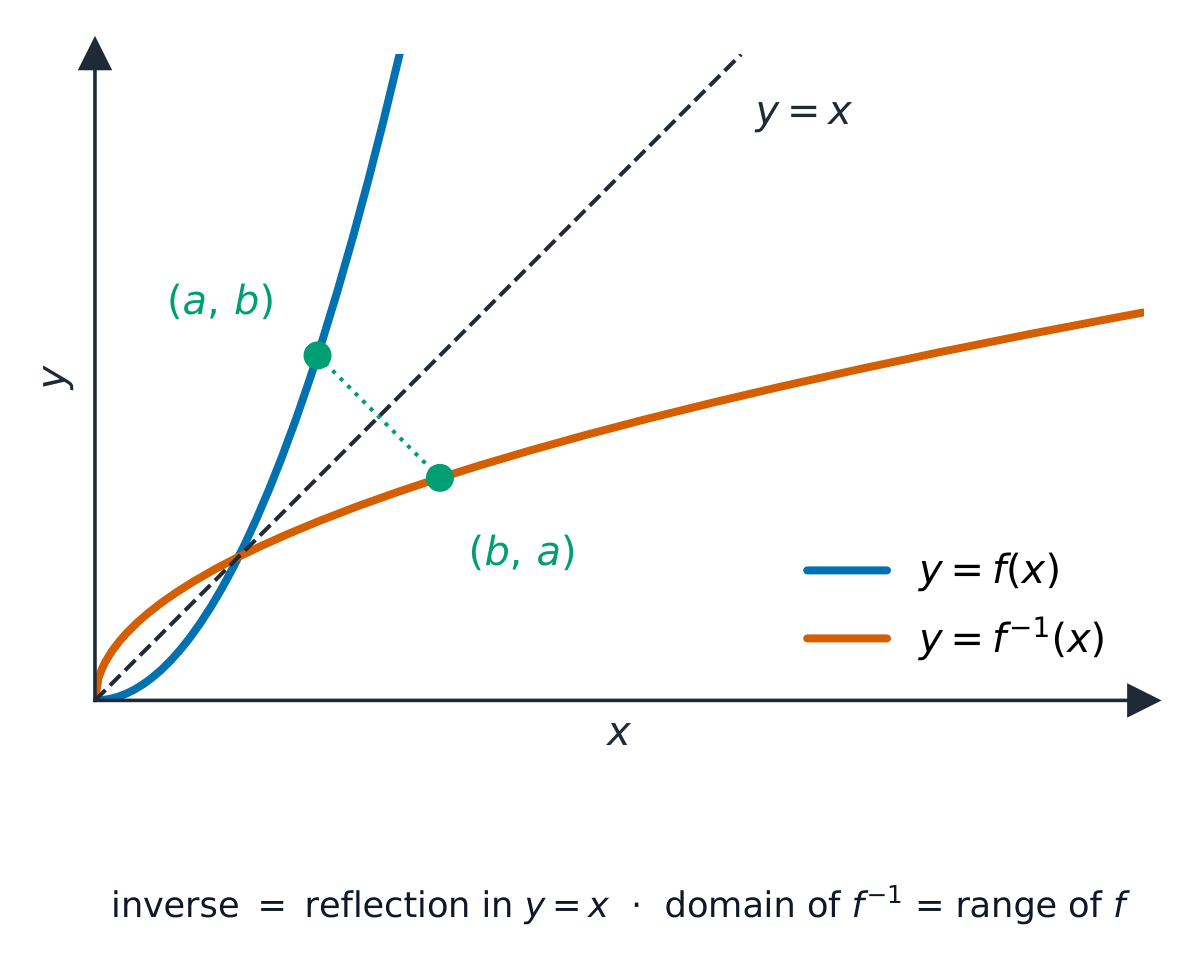


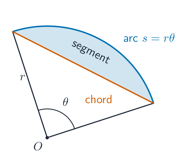


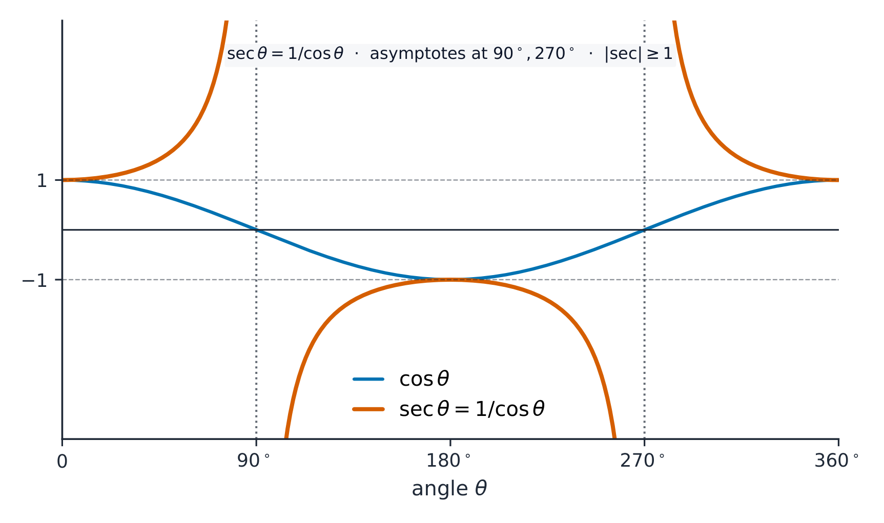


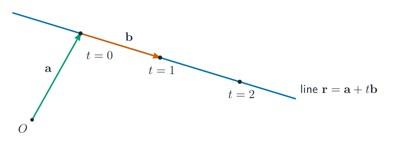


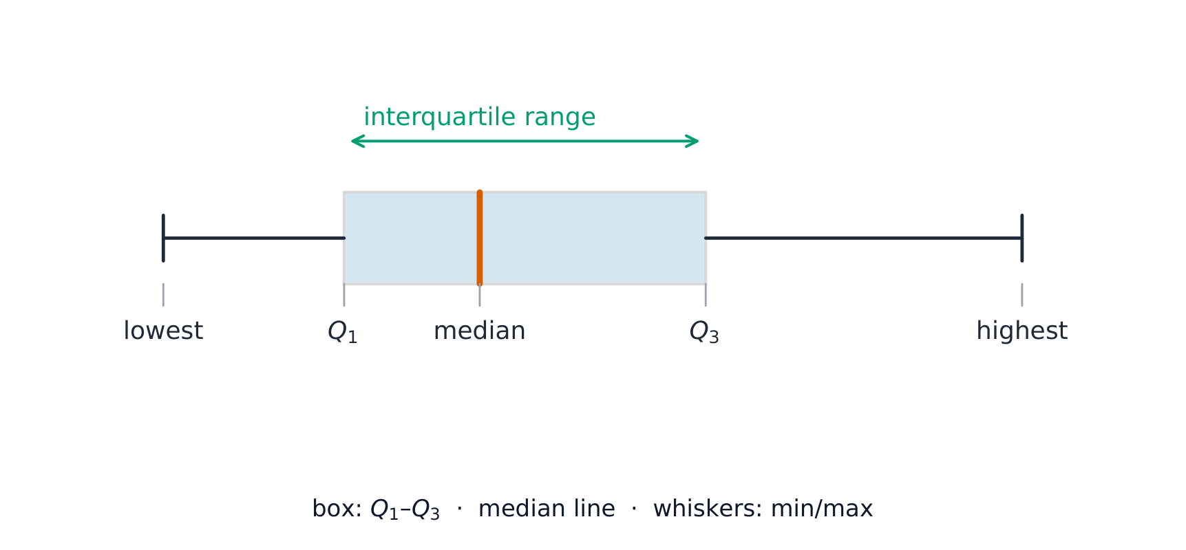

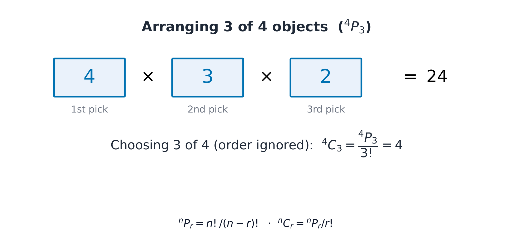

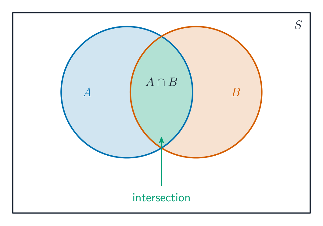
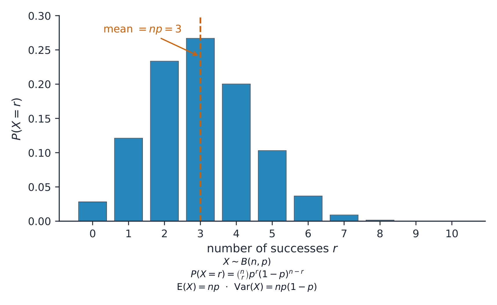

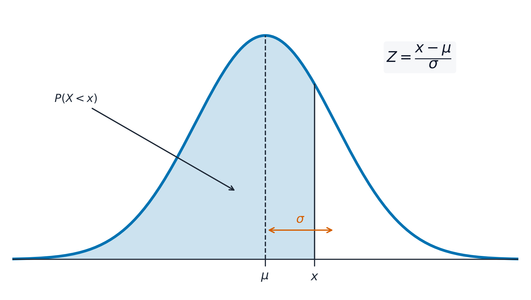
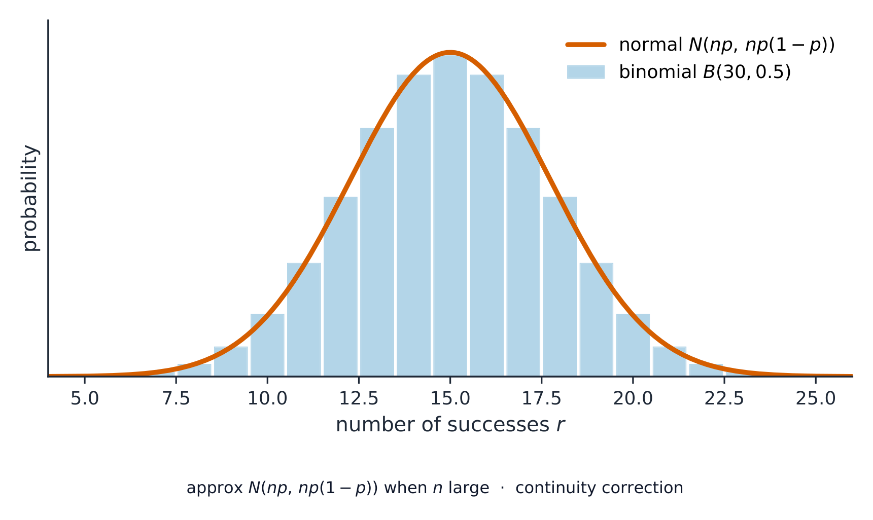

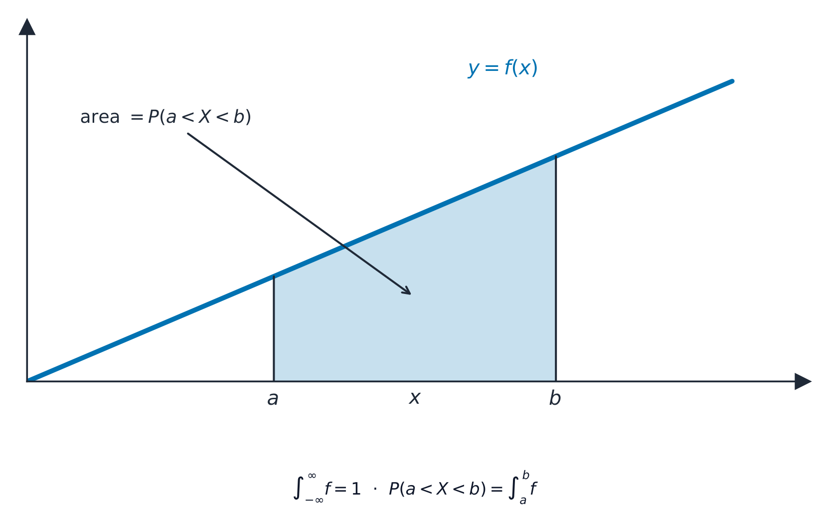


 *Um intervalo de confiança