Observe estes números. Uma bateria pequena diz um ponto cinco volts. Uma bateria de carro diz doze. Uma linha de transmissão de alta tensão transporta quatrocentos mil. A…
English narration · English + 中文 subtitles burned in · Narração em inglês · Legendas em inglês + 中文 gravadas
9.1
Electric Potential Energy · Energia Potencial Elétrica
Syllabus · Programa
English
Learning Objective 9.1.A: Describe the electric potential energy of a system.
9.1.A.1 The electric potential energy of a system of two point charges equals the amount of work required for an external force to bring the point charges to their current positions from infinitely far away.
9.1.A.2 The general form for the electric potential energy between two charged objects is given by the equation
9.1.A.3 The total electric potential energy of a system can be determined by finding the sum of the electric potential energies of the individual interactions between each pair of charged objects in the system.
Português
Objetivo de Aprendizagem 9.1.A: Descrever a energia potencial elétrica de um sistema.
9.1.A.1 A energia potencial elétrica de um sistema de duas cargas pontuais é igual à quantidade de trabalho necessária para que uma força externa traga as cargas pontuais até suas posições atuais desde o infinito.
9.1.A.2 A forma geral para a energia potencial elétrica entre dois objetos carregados é dada pela equação
9.1.A.3 A energia potencial elétrica total de um sistema pode ser determinada encontrando a soma das energias potenciais elétricas das interações individuais entre cada par de objetos carregados no sistema.
Source: College Board AP Course and Exam Description · Fonte: College Board AP Course and Exam Description
English
When you push two like charges together, you do work 功 against the electric force. That work is stored by the pair as electric potential energy 电势能:
$U_E$ is defined as the work an external force must do to bring the charges from infinitely far away to a distance $r$ apart. The signs carry the physics:
Like charges:$U_E>0$. An outside push was needed to bring them together. If released, they fly apart, and the stored energy becomes kinetic energy 动能.
Opposite charges:$U_E<0$. The pair is bound. You must supply $|U_E|$ of work to pull them apart to infinity.
The electric force is a conservative force 保守力: the work it does depends only on the start and end points, not the path, and equals $-\Delta U_E$.
For a system 系统 of several charges, add the potential energy of every distinct pair:
Worked example. Three $+2.0\ \mu\text{C}$ charges sit at the corners of an equilateral triangle with sides $0.30\ \text{m}$. Each pair stores $U=\dfrac{kq^2}{r}=\dfrac{(9.0\times10^{9})(2.0\times10^{-6})^2}{0.30}=0.12\ \text{J}$. There are three pairs, so $U_{\text{total}}=3\times0.12\ \text{J}=0.36\ \text{J}$. This is the work needed to assemble the triangle from infinity – and the kinetic energy the charges would share if all three were released.
Português
Quando você empurra duas cargas iguais juntas, você realiza trabalho 功 contra a força elétrica. Esse trabalho é armazenado pelo par como energia potencial elétrica 电势能:
$U_E$ é definido como o trabalho que uma força externa deve realizar para trazer as cargas de muito longe até uma distância $r$ uma da outra. Os sinais carregam a física:
Cargas iguais:$U_E>0$. Um empurrão externo foi necessário para aproximá-las. Se liberadas, elas voarão para longe, e a energia armazenada se tornará energia cinética 动能.
Cargas opostas:$U_E<0$. O par está ligado. Você deve fornecer $|U_E|$ de trabalho para separá-las até o infinito.
A força elétrica é uma força conservativa 保守力: o trabalho que ela realiza depende apenas dos pontos inicial e final, não do caminho, e é igual a $-\Delta U_E$.
Para um sistema 系统 de várias cargas, some a energia potencial de cada par distinto:
Exemplo resolvido. Três cargas $+2.0\ \mu\text{C}$ estão nos vértices de um triângulo equilátero com lados $0.30\ \text{m}$. Cada par armazena $U=\dfrac{kq^2}{r}=\dfrac{(9.0\times10^{9})(2.0\times10^{-6})^2}{0.30}=0.12\ \text{J}$. Há três pares, então $U_{\text{total}}=3\times0.12\ \text{J}=0.36\ \text{J}$. Este é o trabalho necessário para montar o triângulo a partir do infinito – e a energia cinética que as cargas compartilhariam se todas as três fossem liberadas.
9.2
Electric Potential · Potencial Elétrico
Syllabus · Programa
English
Learning Objective 9.2.A: Describe the electric potential due to a configuration of charged objects.
9.2.A.1 Electric potential describes the electric potential energy per unit charge at a point in space.
9.2.A.2 Expressions for the electric potential of charge distributions can be found using integration and the principle of superposition.
9.2.A.2.i The electric potential for single point charge is
Equation:$V = \dfrac{q}{4\pi\varepsilon_0 r}$.
9.2.A.2.ii The electric potential due to multiple point charges can be determined by the principle of scalar superposition of the electric potential due to each of the point charges.
9.2.A.3 The electric potential difference between two points is the change in electric potential energy per unit charge when a test charge is moved between the two points.
Equation:$\Delta V = \dfrac{\Delta U_E}{q}$
9.2.A.4 Electric potential difference may also result from chemical processes that cause positive and negative charges to separate, such as in a battery.
Boundary statement: AP Physics C: Electricity & Magnetism only expects students to use calculus to find the electric potential resulting from the following charge distributions and locations: an infinitely long, uniformly charged wire or cylinder at a distance from its central axis, a thin ring of charge at a location along the axis of the ring, a semicircular arc or part of a semicircular arc at its center, and a finite wire or line charge at a point collinear with the line charge or at a location along its perpendicular bisector.
Learning Objective 9.2.B: Describe the relationship between electric potential and electric field.
9.2.B.1 The value of an electric field component in any direction at a given location is equal to the negative of the spatial rate of change in electric potential at that location.
Equation:$E_x = -\dfrac{dV}{dx}$
9.2.B.2 The change in electric potential between two points can be determined by integrating the dot product of the electric field and the displacement along the path connecting the points.
Equation:$\Delta V = V_b - V_a = -\displaystyle\int_a^b \vec{E}\cdot d\vec{r}$
9.2.B.3 Electric field vector maps and equipotential lines are tools to describe the field produced by a charge or configuration of charges and can be used to predict the motion of charged objects in the field.
9.2.B.3.i Equipotential lines represent lines of equal electric potential. These lines are also referred to as isolines of electric potential.
9.2.B.3.ii Isolines are perpendicular to electric field vectors. An isoline map of electric potential can be constructed from an electric field vector map, and an electric field map may be constructed from an isoline map.
9.2.B.3.iii An electric field vector points in the direction of decreasing potential.
9.2.B.3.iv There is no component of an electric field along an isoline.
Português
Objetivo de Aprendizagem 9.2.A: Descrever o potencial elétrico devido a uma configuração de objetos carregados.
9.2.A.1 O potencial elétrico descreve a energia potencial elétrica por unidade de carga em um ponto do espaço.
9.2.A.2 Expressões para o potencial elétrico de distribuições de carga podem ser encontradas usando integração e o princípio da superposição.
9.2.A.2.i O potencial elétrico para uma única carga pontual é
Equação:$V = \dfrac{q}{4\pi\varepsilon_0 r}$.
9.2.A.2.ii O potencial elétrico devido a múltiplas cargas pontuais pode ser determinado pelo princípio da superposição escalar do potencial elétrico devido a cada uma das cargas pontuais.
9.2.A.3 A diferença de potencial elétrico entre dois pontos é a mudança na energia potencial elétrica por unidade de carga quando uma carga de prova é movida entre os dois pontos.
Equação:$\Delta V = \dfrac{\Delta U_E}{q}$
9.2.A.4 A diferença de potencial elétrico também pode resultar de processos químicos que causam a separação de cargas positivas e negativas, como em uma bateria.
Declaração de Escopo: AP Physics C: Eletricidade e Magnetismo espera apenas que os alunos usem cálculo para encontrar o potencial elétrico resultante das seguintes distribuições de carga e localizações: um fio ou cilindro infinito uniformemente carregado a uma distância de seu eixo central, um anel fino de carga em uma localização ao longo do eixo do anel, um arco semicircular ou parte de um arco semicircular em seu centro, e um fio finito ou linha de carga em um ponto colinear com a linha de carga ou em uma localização ao longo de sua bissetriz perpendicular.
Objetivo de Aprendizagem 9.2.B: Descrever a relação entre potencial elétrico e campo elétrico.
9.2.B.1 O valor de um componente do campo elétrico em qualquer direção em uma localização dada é igual ao negativo da taxa espacial de mudança no potencial elétrico nessa localização.
Equação:$E_x = -\dfrac{dV}{dx}$
9.2.B.2 A mudança no potencial elétrico entre dois pontos pode ser determinada integrando o produto escalar do campo elétrico e o deslocamento ao longo do caminho conectando os pontos.
Equação:$\Delta V = V_b - V_a = -\displaystyle\int_a^b \vec{E}\cdot d\vec{r}$
9.2.B.3 Mapas de vetores de campo elétrico e linhas equipotenciais são ferramentas para descrever o campo produzido por uma carga ou configuração de cargas e podem ser usadas para prever o movimento de objetos carregados no campo.
9.2.B.3.i Linhas equipotenciais representam linhas de igual potencial elétrico. Essas linhas também são referidas como isolinhas de potencial elétrico.
9.2.B.3.ii Isolinas são perpendiculares aos vetores do campo elétrico. Um mapa de isolinhas de potencial elétrico pode ser construído a partir de um mapa de vetores de campo elétrico, e um mapa de campo elétrico pode ser construído a partir de um mapa de isolinhas.
9.2.B.3.iii Um vetor de campo elétrico aponta na direção de diminuição do potencial.
9.2.B.3.iv Não há componente de um campo elétrico ao longo de uma isolinha.
Source: College Board AP Course and Exam Description · Fonte: College Board AP Course and Exam Description
English
Electric potential 电势 is electric potential energy per unit charge at a point in space. It is measured in volts ($1\ \text{V}=1\ \text{J/C}$):
Potential is a scalar 标量: it has a sign but no direction. This makes $V$ far easier to work with than the field $\vec{E}$. For several point charges 点电荷, use scalar superposition 叠加 – add the potentials with their signs:
Worked example. The potential $0.10\ \text{m}$ from a $+3.0\ \text{nC}$ point charge is $V=\dfrac{kq}{r}=\dfrac{9.0\times10^{9}(3.0\times10^{-9})}{0.10}=270\ \text{V}$. Now add a $-3.0\ \text{nC}$ charge $0.30\ \text{m}$ from the same point: it contributes $\dfrac{9.0\times10^{9}(-3.0\times10^{-9})}{0.30}=-90\ \text{V}$, so the total is $270-90=180\ \text{V}$. Just a signed sum – no vector components to resolve.
Continuous charge distributions
For a continuous charge distribution 连续电荷分布, cut it into small pieces $dq$, treat each piece as a point charge, and integrate 积分:
This is a scalar integral, so it is usually much easier than the field integral. AP expects you to handle four shapes with calculus: a thin ring (at a point on its axis), an arc (at its centre), a finite line or wire (collinear, or on its perpendicular bisector), and an infinitely long wire or cylinder (at a distance from its axis).
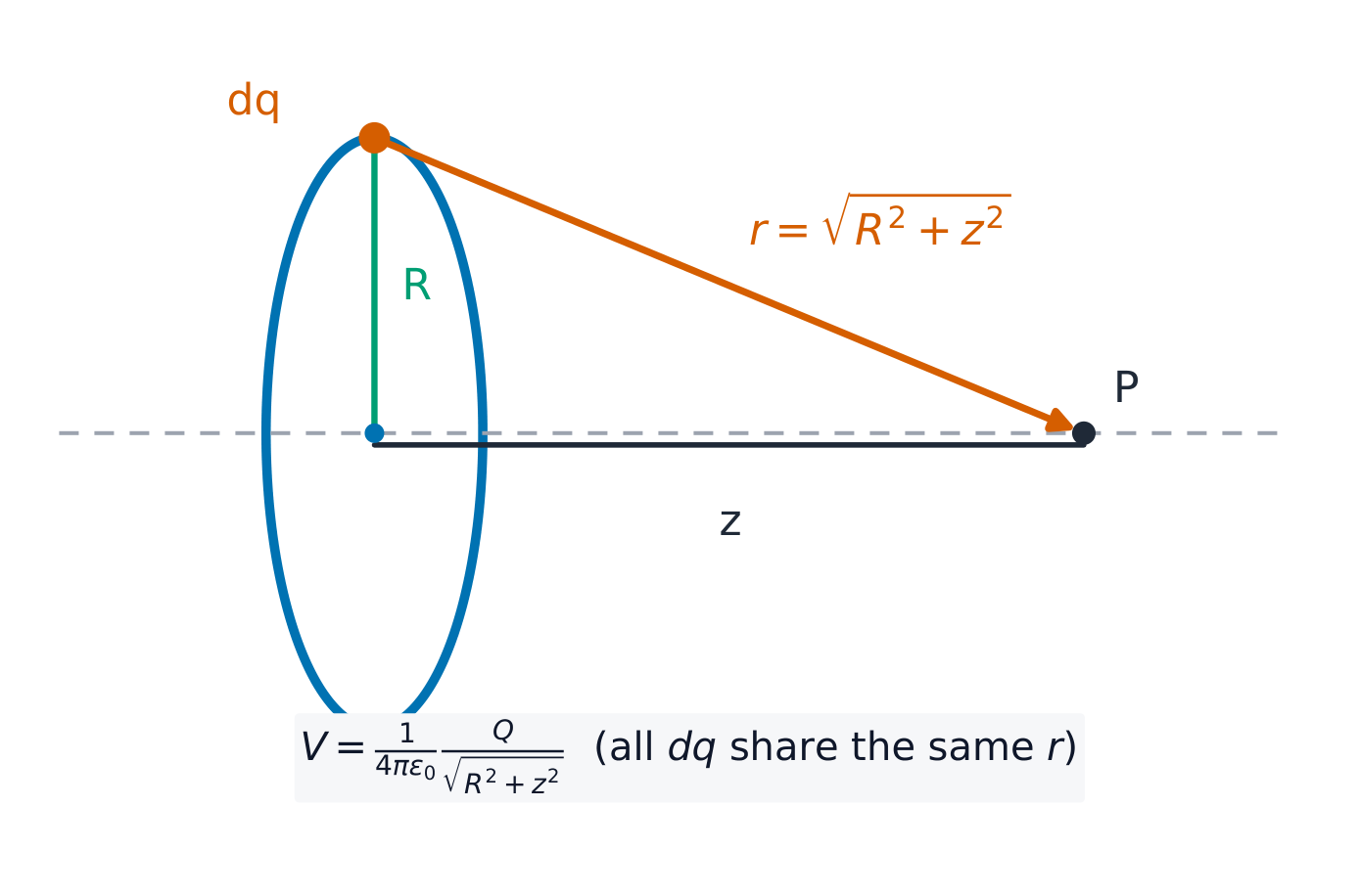
Worked example (ring of charge). A thin ring of radius $R$ carries total charge $Q$. For a point $P$ on the axis a distance $z$ from the centre, every element $dq$ sits at the same distance $r=\sqrt{R^2+z^2}$ from $P$. The distance is constant, so it comes out of the integral:
On an FRQ, say that $r$ is the same for every element – that statement is the marked step. The same idea gives $V=kQ/R$ at the centre of any arc, whatever its angle.
From potential to field
Potential and field contain the same information, linked by a derivative in each direction and by a path integral:
The field is the negative gradient 梯度 of the potential: $\vec{E}$ points from high potential to low potential, "downhill". Where $V$ changes quickly, the field is strong.
Worked example. Along the $x$-axis, $V(x)=3x^{2}-2x$ (volts, with $x$ in metres). Then $E_x=-\dfrac{dV}{dx}=2-6x\ \text{V/m}$. At $x=0.50\ \text{m}$, $E_x=-1.0\ \text{V/m}$: the field there points in the $-x$ direction.
The potential difference 电势差 between two points is the change in potential energy per unit charge moved between them: $\Delta V=\Delta U_E/q$. A battery makes a potential difference chemically: reactions inside separate positive from negative charge and hold the terminals a fixed $\Delta V$ apart.
Equipotential maps
An equipotential 等势面 line (also called an isoline 等值线) joins points that share the same potential. Four rules let you read any map:
Isolines are perpendicular 垂直 to field lines 电场线 everywhere they cross.
$\vec{E}$ points from high $V$ to low $V$ – never along an isoline. Moving a charge along an isoline takes no work.
Closely spaced isolines mean a strong field: $E\approx-\Delta V/\Delta x$.
You can sketch the field map from an isoline map, and the isoline map from a field map.
Exam skill. Given a map with isolines every $10\ \text{V}$ spaced about $2\ \text{cm}$ apart, estimate $E\approx\dfrac{10}{0.02}=500\ \text{V/m}$, pointing from the higher-value line to the lower one. The work an external agent does moving a charge $q$ slowly from $A$ to $B$ is $W=q(V_B-V_A)$ – the path taken does not matter.
Português
Potencial elétrico 电势 é energia potencial elétrica por unidade de carga em um ponto no espaço. É medido em volts ($1\ \text{V}=1\ \text{J/C}$):
O potencial é uma escalar 标量: tem um sinal, mas nenhuma direção. Isso torna $V$ muito mais fácil de manipular do que o campo $\vec{E}$. Para várias cargas pontuais 点电荷, use sobreposição escalar 叠加 – some os potenciais com seus sinais:
Exemplo resolvido. O potencial $0.10\ \text{m}$ de uma carga pontual $+3.0\ \text{nC}$ é $V=\dfrac{kq}{r}=\dfrac{9.0\times10^{9}(3.0\times10^{-9})}{0.10}=270\ \text{V}$. Agora adicione uma carga $-3.0\ \text{nC}$$0.30\ \text{m}$ do mesmo ponto: ela contribui com $\dfrac{9.0\times10^{9}(-3.0\times10^{-9})}{0.30}=-90\ \text{V}$, então o total é $270-90=180\ \text{V}$. Apenas uma soma com sinal – sem componentes vetoriais para resolver.
Distribuições de carga contínuas
Para uma distribuição de carga contínua 连续电荷分布, divida-a em pequenas peças $dq$, trate cada peça como uma carga pontual e integre 积分:
Esta é uma integral escalar, portanto geralmente é muito mais fácil do que a integral de campo. A AP espera que você lidasse com quatro formas usando cálculo: um anel fino (em um ponto em seu eixo), um arco (em seu centro), uma linha ou fio finito (colineal, ou em sua bissetriz perpendicular) e um fio ou cilindro infinito (a uma distância de seu eixo).
Um anel de carga: cada elemento dq está na mesma distância de um ponto do eixo
Exemplo resolvido (anel de carga). Um anel fino de raio $R$ carrega carga total $Q$. Para um ponto $P$ no eixo a uma distância $z$ do centro, cada elemento $dq$ está à mesma distância $r=\sqrt{R^2+z^2}$ de $P$. A distância é constante, então sai da integral:
Em uma FRQ, diga que $r$ é o mesmo para cada elemento – essa afirmação é o passo avaliado. A mesma ideia dá $V=kQ/R$ no centro de qualquer arco, independentemente do seu ângulo.
De potencial a campo
Potencial e campo contêm a mesma informação, ligados por uma derivada em cada direção e por uma integral de caminho:
O campo é o negativo gradiente 梯度 do potencial: $\vec{E}$ aponta de alto potencial para baixo potencial, "montanha abaixo". Onde $V$ muda rapidamente, o campo é forte.
Exemplo resolvido. Ao longo do eixo $x$, $V(x)=3x^{2}-2x$ (volts, com $x$ em metros). Então $E_x=-\dfrac{dV}{dx}=2-6x\ \text{V/m}$. Em $x=0.50\ \text{m}$, $E_x=-1.0\ \text{V/m}$: o campo lá aponta na direção $-x$.
Em um campo uniforme o potencial cai constantemente com a distância
A diferença de potencial 电势差 entre dois pontos é a mudança na energia potencial por unidade de carga movida entre eles: $\Delta V=\Delta U_E/q$. Uma bateria cria uma diferença de potencial quimicamente: reações internas separam cargas positivas de negativas e mantêm os terminais fixamente $\Delta V$ separados.
O potencial próximo a uma carga pontual varia como 1/r
Mapas equipotenciais
Uma linha equipotencial 等势面 (também chamada de isolinha 等值线) une pontos que compartilham o mesmo potencial. Quatro regras permitem ler qualquer mapa:
Isolinhas são perpendiculares 垂直 às linhas de campo 电场线 em todos os pontos onde cruzam.
$\vec{E}$ aponta de alto $V$ para baixo $V$ – nunca ao longo de uma isolinha. Mover uma carga ao longo de uma isolinha não requer trabalho.
Isolinhas próximas significam um campo forte: $E\approx-\Delta V/\Delta x$.
Você pode esboçar o mapa de campo a partir de um mapa de isolinhas, e o mapa de isolinhas a partir de um mapa de campo.
Linhas equipotenciais ao redor de um dipolo cruzam as linhas de campo em ângulos retos
Habilidade de prova. Dado um mapa com isolinhas a cada $10\ \text{V}$ espaçadas cerca de $2\ \text{cm}$, estime $E\approx\dfrac{10}{0.02}=500\ \text{V/m}$, apontando da linha de valor maior para a menor. O trabalho que um agente externo realiza movendo uma carga $q$ lentamente de $A$ para $B$ é $W=q(V_B-V_A)$ – o caminho percorrido não importa.
Linhas de transmissão de alta tensão: energia potencial elétrica é convertida e transmitida como corrente em alta tensão
Explore · Explorar
Linhas de campo e o potencial ao redor de uma carga
Potencial elétrico é a energia por unidade de carga. Ele diminui com a distância de uma carga positiva; as linhas de campo apontam do potencial alto para o baixo.
Conservation of Electric Energy · Conservação de Energia Elétrica
Syllabus · Programa
English
Learning Objective 9.3.A: Describe changes in a system due to a difference in electric potential between two locations.
9.3.A.1 When a charged object moves between two locations with different electric potentials, the resulting change in the electric potential energy of the object-field system is given by the following equation.
Equation:$\Delta U_E = q\Delta V$
9.3.A.2 The movement of a charged object between two points with different electric potentials results in a change in kinetic energy of the object consistent with the conservation of energy.
Português
Objetivo de Aprendizagem 9.3.A: Descrever as mudanças em um sistema devido a uma diferença de potencial elétrico entre dois locais.
9.3.A.1 Quando um objeto carregado se move entre dois locais com diferentes potenciais elétricos, a mudança resultante na energia potencial elétrica do sistema objeto-campo é dada pela seguinte equação.
Equação:$\Delta U_E = q\Delta V$
9.3.A.2 O movimento de um objeto carregado entre dois pontos com diferentes potenciais elétricos resulta em uma mudança na energia cinética do objeto consistente com a conservação da energia.
Source: College Board AP Course and Exam Description · Fonte: College Board AP Course and Exam Description
English
When a charge $q$ moves between two points that differ in potential by $\Delta V$, the potential energy of the charge–field system changes by
$$\Delta U_E=q\,\Delta V.$$
If only the electric force acts, total energy is conserved, so the kinetic energy changes by the opposite amount:
$$\Delta K=-\Delta U_E=-q\,\Delta V.$$
Watch the two signs together: a positive charge speeds up when it moves to lower potential, while a negative charge speeds up when it moves to higher potential. Both are just the system trading potential energy for kinetic energy. This is how particle accelerators give charged particles their energy, and it underlies energy analysis in circuits.
Worked example. A proton ($q=1.6\times10^{-19}\ \text{C}$, $m=1.67\times10^{-27}\ \text{kg}$) starts at rest and is accelerated through a potential drop of $500\ \text{V}$ (it moves to lower potential, so $\Delta V=-500\ \text{V}$ and $\Delta K=-q\,\Delta V=+8.0\times10^{-17}\ \text{J}$). Setting $\Delta K=\tfrac12 mv^2$:
Exam skill. Choose energy methods, not kinematics, whenever the field is non-uniform or the path curves: only the end-point potentials matter. A typical FRQ chain is $q\,\Delta V \to \Delta K \to v$, with one line of justification: "the electric force is conservative, so energy is conserved."
Português
Quando uma carga $q$ se move entre dois pontos que diferem em potencial por $\Delta V$, a energia potencial do sistema carga-campo muda por
$$\Delta U_E=q\,\Delta V.$$
Se apenas a força elétrica atua, a energia total é conservada, então a energia cinética muda pela quantidade oposta:
$$\Delta K=-\Delta U_E=-q\,\Delta V.$$
Observe os dois sinais juntos: uma carga positiva acelera quando se move para baixo potencial, enquanto uma carga negativa acelera quando se move para alto potencial. Ambos são apenas o sistema trocando energia potencial por energia cinética. Esta é a forma como aceleradores de partículas dão energia a partículas carregadas, e fundamenta a análise energética em circuitos.
Exemplo resolvido. Um próton ($q=1.6\times10^{-19}\ \text{C}$, $m=1.67\times10^{-27}\ \text{kg}$) começa em repouso e é acelerado através de uma queda de potencial de $500\ \text{V}$ (ele se move para baixo potencial, então $\Delta V=-500\ \text{V}$ e $\Delta K=-q\,\Delta V=+8.0\times10^{-17}\ \text{J}$). Igualando $\Delta K=\tfrac12 mv^2$:
Habilidade de prova. Escolha métodos energéticos, não cinemática, sempre que o campo for não uniforme ou a trajetória curvar: apenas os potenciais dos pontos finais importam. Uma cadeia típica de FRQ é $q\,\Delta V \to \Delta K \to v$, com uma linha de justificativa: "a força elétrica é conservativa, então a energia é conservada."
9.3
Exam tips · Dicas de prova
English
Relate field and potential by $V=-\int \vec E\cdot d\vec l$ and $\vec E=-\nabla V$ (in 1-D, $E_x=-\tfrac{dV}{dx}$).
Potential is a scalar — add contributions with signs, no vector components needed.
Potential energy of a pair is $U=\tfrac{1}{4\pi\varepsilon_0}\tfrac{q_1 q_2}{r}$; use energy conservation for a charge's speed.
Know that no work is done moving along an equipotential, which is perpendicular to $\vec E$.
Choose the zero of potential (usually infinity) and state it.
Português
Relacione campo e potencial por $V=-\int \vec E\cdot d\vec l$ e $\vec E=-\nabla V$ (em 1-D, $E_x=-\tfrac{dV}{dx}$).
Potencial é uma escalar — some contribuições com sinais, sem componentes vetoriais necessárias.
Energia potencial de um par é $U=\tfrac{1}{4\pi\varepsilon_0}\tfrac{q_1 q_2}{r}$; use conservação de energia para a velocidade de uma carga.
Saiba que nenhum trabalho é realizado movendo-se ao longo de uma equipotencial, que é perpendicular a $\vec E$.
Escolha o zero do potencial (geralmente o infinito) e declar-o.
Interactive lessons on this topic · Aulas interativas sobre este tópico
Work through it step by step, with instant-check exercises. · Passe por ele passo a passo, com exercícios de verificação instantânea.
Pick one and the site follows you — notes, papers, videos and practice all open on it. · Escolha uma e o site te seguirá — notas, provas, vídeos e prática abrirão nela.
Type to search notes, lessons, code, vocabulary and past-paper questions across every subject. · Digite para pesquisar notas, aulas, código, vocabulário e questões de provas anteriores em todas as disciplinas.