| Learning Objective | Essential Knowledge |
|---|---|
2.1.A |
|
2.1.B |
|
Exponential and Logarithmic Functions
AP Precalculus · Topic 2
 14:05
Exponential & Logarithmic Functions
Here are two ways for a quantity to grow. The blue line grows steadily, adding the same amount every step. The other one is doubling — multiplying by the same…
English narration · English + 中文 subtitles burned in
2.1
Change in Arithmetic and Geometric Sequences

Syllabus
Source: College Board AP Course and Exam Description
A sequence 数列 is a function from the whole numbers to the real numbers, so its graph is discrete points, not a curve.
- An arithmetic sequence 等差数列 has a common difference 公差 $d$ (a constant rate of change): $a_n = a_0 + dn$, or from a known term, $a_n = a_k + d(n-k)$.
- A geometric sequence 等比数列 has a common ratio 公比 $r$ (a constant proportional change): $g_n = g_0\,r^{\,n}$, or $g_n = g_k\,r^{\,(n-k)}$.
An increasing arithmetic sequence changes by the same positive amount each step. For a positive geometric starting value and $r>1$, successive increases get larger. A negative starting value with $r>1$ instead becomes more negative; with a positive start and $0<r<1$, the sequence decreases toward zero.
Worked example. An arithmetic sequence with $a_0=3$ and $d=5$ has $a_4=3+5(4)=23$. A geometric sequence with $g_0=2$ and $r=3$ has $g_4=2\cdot3^4=162$ – addition versus multiplication makes the geometric one pull far ahead.
Check the starting index. The example above numbers its first term 0. If 3 is instead called $a_1$, the same arithmetic list is $a_n=3+5(n-1)$ and its fourth numbered term is $a_4=18$. The original $a_4=23$ is the fifth listed value. Count the number of changes from the known term, rather than memorising one exponent.
An explicit sequence rule 数列显式公式 is a formula that gives a term directly from its index. A recursive sequence rule 数列递推公式 is a starting value together with a formula for the next term.
Worked example: recursive form. Start with $g_0=2$, then use $g_n=3g_{n-1}$ for $n\ge1$. This gives the same $g_n=2\cdot3^n$ as the original worked example.
A second comparison. With first terms numbered 1, consider $u_n=2+2(n-1)$ and $v_n=2^{n-1}$. At term 5 the values are 10 and 16. Their first five terms are $2,4,6,8,10$ and $1,2,4,8,16$. With a positive geometric starting value and $r>1$, eventual dominance over a fixed arithmetic rule follows from the growth rates, not from seeing a few plotted terms.
Try it. An arithmetic sequence has $a_4=17$ and $d=3$. Find $a_9$. A geometric sequence has $g_2=6$ and $r=2$. Find $g_6$. Use $n-k$ changes in each case.
Check. $a_9=17+3(9-4)=32$; $g_6=6\cdot2^{6-2}=96$.
Explore
Compare two stated sequence rules
First terms are numbered 1. Compare adding 2 from a first term of 2 with doubling from a first term of 1; term 5 gives 10 and 16.
Vocabulary
Train
| English |
|---|
| sequence/ˈsiːkwəns/ |
| arithmetic sequence/əˈrɪθmətɪk ˈsiːkwəns/ |
| common difference/ˈkɒmən ˈdɪfrəns/ |
| geometric sequence/ˌdʒiːəʊˈmetrɪk ˈsiːkwəns/ |
| common ratio/ˈkɒmən ˈreɪʃɪəʊ/ |
| explicit sequence rule |
| recursive sequence rule |
2.2
Change in Linear and Exponential Functions

Syllabus
| Learning Objective | Essential Knowledge |
|---|---|
2.2.A |
|
Source: College Board AP Course and Exam Description
A quantity is 12 at input 2. A linear model adds 3 per input unit, while an exponential model multiplies by 1.5 per unit. At input 4 they predict $12+3(4-2)=18$ and $12(1.5)^{4-2}=27$. Both models pass through the known point, but one observation does not choose between them.
- A linear function 线性函数 $f(x)=y_0+m(x-x_0)$ has constant output differences over equal input intervals. From two distinct inputs, $m=(y_2-y_1)/(x_2-x_1)$.
- For positive outputs, an exponential model $f(x)=y_0b^{x-x_0}$ has constant output ratios over equal input intervals. From two observations, $b=(y_2/y_1)^{1/(x_2-x_1)}$. Attach the input unit to this factor.
Compare equal intervals. At inputs $0,2,4$, outputs $5,9,13$ have a constant two-unit difference of 4, so the linear slope is 2 per unit. Outputs $5,20,80$ have a constant two-unit factor of 4, so the positive per-unit factor is 2. Ratios or differences from unequal input intervals cannot be compared directly.
- Linear functions $f(x)=b+mx$ mirror arithmetic sequences – an initial value plus repeated addition of the slope $m$. Point form: $f(x)=y_i+m(x-x_i)$.
- Exponential functions $f(x)=ab^x$ mirror geometric sequences – an initial value times repeated multiplication by the base $b$. Point form: $f(x)=y_i\,b^{\,(x-x_i)}$.
A domain 定义域 states the permitted inputs. Sequences use discrete indices; a continuous function model can also use intermediate inputs, but that requires a modeling assumption. A 20% increase followed by a 20% decrease multiplies by $1.2(0.8)=0.96$, leaving a 4% decrease overall. Both percentages refer to the value just before their change, not to a common fixed amount.
Try it. A positive exponential model passes through $(2,18)$ and $(5,144)$. Find its per-unit factor and value at input 0. A linear model passes through the same points; find its slope.
Check. $b^3=144/18=8$, so $b=2$ and $f(0)=18/2^2=4.5$. The linear slope is $(144-18)/(5-2)=42$ per input unit.
Explore
Changes from a shared known point
$\begin{aligned}L(t)&=y_i+m(t-2)\\E(t)&=y_i r^{t-2}\end{aligned}$
Start from (2,10), with slope 3 and unit factor 2. Compare additive differences with multiplicative ratios over the same input gap.
Vocabulary
Train
| English |
|---|
| linear function/ˈlɪnɪə ˈfʌŋkʃn/ |
| domain/dəˈmeɪn/ |
2.3
Exponential Functions

Syllabus
| Learning Objective | Essential Knowledge |
|---|---|
2.3.A |
|
Source: College Board AP Course and Exam Description
The general exponential function 指数函数 is $f(x)=ab^x$, with initial value 初始值 $a\ne0$ and base 底数 $b>0$, $b\ne1$. Its mathematical domain is all real numbers, although a context may use only part of it.
For $a>0$, $b>1$ gives exponential growth 指数增长 and $0<b<1$ gives exponential decay 指数衰减. A negative $a$ reflects the graph across the horizontal axis. The four cases are:
| Start | Base | Direction | Concavity |
|---|---|---|---|
| $a>0$ | $b>1$ | Increasing | Up |
| $a>0$ | $0<b<1$ | Decreasing | Up |
| $a<0$ | $b>1$ | Decreasing | Down |
| $a<0$ | $0<b<1$ | Increasing | Down |
The outputs never change sign. The range is $y>0$ for $a>0$ and $y<0$ for $a<0$. The horizontal asymptote is $y=0$: for $b>1$ it is approached as $x\to-\infty$, while for $0<b<1$ it is approached as $x\to\infty$. At the opposite end, the magnitude increases without bound.
A nonconstant exponential is strictly monotonic and has no turning points or inflection points. On a closed interval its maximum and minimum occur at the endpoints. The cases $a=0$ or $b=1$ give constants and are separate from this nonconstant family. For a shifted model $f(x)=k+ab^{x-h}$, apply these tests to $f(x)-k$; the asymptote is $y=k$.
Explore
Exponential sign, range and direction
f(x) = a·bˣ
For f(x)=3·4ˣ, f(2)=48. Use both the coefficient sign and the base to distinguish increasing, decreasing and constant cases.
Vocabulary
Train
| English |
|---|
| exponential function/ˌekspəˈnenʃl ˈfʌŋkʃn/ |
| initial value/ɪˈnɪʃl ˈvæljuː/ |
| base/beɪs/ |
| exponential growth/ˌekspəˈnenʃl ɡrəʊθ/ |
| exponential decay/ˌekspəˈnenʃl dɪˈkeɪ/ |
2.4
Exponential Function Manipulation
Syllabus
| Learning Objective | Essential Knowledge |
|---|---|
2.4.A |
|
Source: College Board AP Course and Exam Description
For a positive base, exponent rules relate equivalent expressions. Keep a negative coefficient separate from a base: $-2^x$ means $-(2^x)$, whereas $(-2)^x$ is not real for every real input.
- Product: $b^u b^v=b^{u+v}$. For example, $2^{x+3}=8(2^x)$ is both a shift left by 3 of $2^x$ and a vertical stretch by 8.
- Power: $(b^u)^v=b^{uv}$. Thus $2^{3x}=8^x$ compresses the graph horizontally by a factor of 3; $2^{x/3}$ stretches it horizontally by 3.
- Negative exponent: $b^{-x}=1/b^x=(1/b)^x$. This reflects the graph of $b^x$ across the vertical axis; it is not a negative output.
- Unit-fraction exponent: $b^{1/k}=\sqrt[k]{b}$ for a positive integer $k$; this is the $k$th root 方根. More generally, $b^{m/k}=\sqrt[k]{b^m}$.
Worked example: preserve the order of transformations. For $F(x)=-3\cdot2^{2(x-1)}+5$, use the adjusted input $2(x-1)$, multiply the exponential output by $-3$, then add 5. The asymptote is $y=5$, the range is $y<5$, and $F(1)=-3+5=2$. Doubling the adjusted input is not the same as doubling the whole function output.
Change the input unit. Since $b^x=e^{x\ln b}$, $45(2)^t=45e^{(\ln2)t}$. If $u$ counts minutes instead of hours, $t=u/60$ and the exponent is $(\ln2)u/60$. An equivalent form changes the coefficient in the exponent with the input units.
Try it. Rewrite $3\cdot4^{x-2}$ as $A\cdot4^x$, and rewrite $2^{x/2}$ with exponent $x$.
Check. $A=3/4^2=3/16$; $2^{x/2}=(\sqrt2)^x$.
Explore
Exponent shifts and input dilations
$b^{cx+k}=b^k(b^c)^x$
Compare shifted-exponent and coefficient/new-base forms. The default is $2^{2x-1}=0.5(4)^x$.
Vocabulary
Train
| English |
|---|
| root/ruːt/ |
2.5
Exponential Function Context and Data Modeling
Syllabus
| Learning Objective | Essential Knowledge |
|---|---|
2.5.A |
|
Source: College Board AP Course and Exam Description
A culture has 180 cells at hour 2 and 1440 cells at hour 5. An exponential model assumes a constant proportion of change over equal-length input intervals. The observations span three hours, so their ratio is a three-hour factor, not an hourly factor.
Worked example: construct a model from two observations
For positive counts, write $N(t)=ab^t$ with $a>0$ and $b>0$. Substitute the observations and divide to remove $a$:
$$\begin{aligned}
180&=ab^2,\\
1440&=ab^5,\\
b^{5-2}&=\frac{1440}{180}=8,\\
b&=\sqrt[3]{8}=2,\\
a&=\frac{180}{2^2}=45.
\end{aligned}$$
Thus $N(t)=45(2)^t$. Check both observations: $N(2)=180$ and $N(5)=1440$. At hour 4 it predicts $N(4)=720$. The initial value is 45 at the chosen hour 0, not the first recorded count of 180. It is inferred, rather than measured.
Keep the input interval attached to the factor
The hourly factor 2 means a 100% increase per hour. The three-hour factor 8 means a 700% increase across three hours. If $u=t-2$ counts hours since the first observation, use $N=180(2)^u$. If $s=t/3$ counts three-hour periods from the original origin, use $N=45(8)^s$. These are descriptions of the same model with different input labels or units.
Worked example: adjust for a nonzero background. A drink cools in a room held at 20°C. The raw temperature ratios are not constant, but subtracting the baseline 基准值 of 20 reveals a proportional pattern:
| Time (hours) | Temperature (°C) | Temperature minus 20 (°C) |
|---|---|---|
| 0 | 100 | 80 |
| 1 | 60 | 40 |
| 2 | 40 | 20 |
| 3 | 30 | 10 |
A baseline is the fixed background value from which the modeled difference is measured. The differences halve each hour, giving $T(t)=20+80(0.5)^t$. Using just hours 0 and 2, the adjusted ratio gives
$$\begin{aligned}
b^2&=\frac{40-20}{100-20}=\frac14,\\
b&=\frac12,\\
T(0)&=20+80=100.
\end{aligned}$$
Check the distinction: For a shifted model $y=c+ab^t$, the initial output is $c+a$, not $a$. The baseline $c$ must be known or separately estimated: two readings alone do not determine all three parameters. Subtract a positive background, or equivalently add its negative, before looking for constant ratios. Here the model approaches 20°C rather than zero. Counting time from the hour-2 reading gives the equivalent form $T=20+20(0.5)^u$, with $u=t-2$.
Natural-base form and noisy data. The natural base 自然底数 is $e\approx2.718$. Since $b=e^{\ln b}$, the same culture model is $N=45e^{(\ln2)t}$. In $ae^{kt}$, $k=\ln b$; it is not the ordinary fractional increase $b-1$. Here $k\approx0.693$ per hour, while the one-hour increase is 100%.
Use exponential regression 指数回归 with technology when measurements are noisy, then check the predictions against all the data. A log-linear fit regresses $\ln y$ on the input for positive $y$; with a known baseline, apply it to $\ln(y-c)$ only when $y-c>0$. A two-point fit can be exact even when an exponential is unsuitable. Population forecasts need continued growth conditions; the cooling model needs a stable room temperature. Justify predictions beyond the observations.
Try it. A culture has 81 cells at hour 3 and 729 cells at hour 5. Assuming $N=ab^t$, find the hourly factor, the inferred count at hour 0 and the prediction at hour 4. For $T(t)=18+62(0.5)^t$, find the initial temperature and the temperature at hour 2.
Check. For the culture, $b^2=729/81=9$, so $b=3$ and $a=81/3^3=3$. Hence $N(4)=3(3)^4=243$ cells. For the drink, $T(0)=80$°C and $T(2)=18+62/4=33.5$°C.
Worked example: two points. An exponential model $f(x)=ab^x$ passes through $(1,6)$ and $(3,54)$. Divide the two equations so that $a$ cancels:
$$\frac{ab^3}{ab^1}=\frac{54}{6} \;\Rightarrow\; b^2=9 \;\Rightarrow\; b=3 \ (b>0).$$
Then $ab=6$ gives $a=2$, so $f(x)=2\cdot 3^x$. Check: $f(3)=2\cdot27=54$.
Explore
Construct a model from observed intervals
The culture has 180 cells at hour 2 and 1440 at hour 5. Compare the three-hour and hourly factors, then examine cooling above a baseline.
Vocabulary
Train
| English |
|---|
| baseline/ˈbeɪslaɪn/ |
| natural base/ˈnætʃərəl beɪs/ |
| exponential regression/ˌekspəˈnenʃl rɪˈɡreʃn/ |
2.6
Competing Function Model Validation
Syllabus
| Learning Objective | Essential Knowledge |
|---|---|
2.6.A |
|
2.6.B |
|
Source: College Board AP Course and Exam Description
Several families can appear close to the same data over a short interval. Construct candidates on the same observations, compare their errors, and use context to judge their applicability.
Worked example: compare three regressions. A video has 100, 151, 224, 339 and 505 views on days $x=0,1,2,3,4$. Technology gives these fitted models, with displayed coefficients rounded:
$$\begin{aligned}
L(x)&=64.2+99.8x,\\
Q(x)&\approx103.0571\\
&\quad+22.0857x\\
&\quad+19.4286x^2,\\
E(x)&\approx100.2264(1.498927)^x.
\end{aligned}$$
The linear and quadratic regressions minimise squared errors in the view counts. This exponential fit uses linear regression of $\ln y$ on $x$, then converts back; it minimises squared log errors. Different calculator fitting methods can give slightly different exponential coefficients. Keep full precision for residual calculations.
A residual 残差 is observed minus predicted. On day 2 the line predicts $L(2)=263.8$, while the observed count is 224:
$$e=224-263.8=-39.8.$$
The negative residual means the line overestimates by 39.8 views. A positive residual means that an observation lies above the model and the model underestimates it. A residual plot 残差图 plots these signed differences against the input, with zero as a reference.
| Day | Observed | Linear residual | Quadratic residual | Exponential residual |
|---|---|---|---|---|
| 0 | 100 | 35.80 | -3.06 | -0.23 |
| 1 | 151 | -13.00 | 6.43 | 0.77 |
| 2 | 224 | -39.80 | -0.94 | -1.19 |
| 3 | 339 | -24.60 | -5.17 | 1.46 |
| 4 | 505 | 41.60 | 2.74 | -0.95 |
Read size and pattern together. The line's residuals are positive at the ends and negative in the middle: a curved pattern suggests it misses the data's shape. Their signed total is zero, although individual errors are large. Adding absolute residuals avoids this cancellation. The totals are 154.8 views for the line, about 18.34 for the quadratic and about 4.59 for the exponential, using full-precision values.
Here the exponential has smaller errors and no clear residual pattern, consistent with roughly constant proportional growth. Pattern-free residuals support a model; five observations do not prove that it is the true rule or that it will forecast well far beyond days 0–4. Sketching the three residual plots from the table makes the comparison clearer than the fitted curves alone.
Use the consequence of an error. If a bus-demand model predicts 48 passengers and 55 arrive, the residual is $55-48=7$: it underestimates demand. A cautious overestimate may be preferable when too few seats would leave people behind. A useful recommendation states the error's direction and size, the interval and the contextual assumptions.
Keep eventual growth separate from present fit. A positive-start exponential with base greater than 1 eventually exceeds any fixed polynomial as the input increases without bound. This fact does not establish which family fits a particular data set best. Decay does not have that positive-growth conclusion, and a polynomial passing through every point can still give poor forecasts outside the data.
Try it. A model predicts 210 when the observed value is 195. Find and interpret the residual. Model A has residuals $6,-4,2$ and model B has $5,5,5$ on the same three observations. Compare their totals of absolute residuals, then name one further validity check.
Check. The residual is $195-210=-15$, so the model overestimates by 15. A totals $6+4+2=12$; B totals $5+5+5=15$. A is better by this measure on these observations. Inspect the residual plot for a pattern and check that the family and prediction interval make sense in context before recommending it.
Explore
Compare three fits on the same five observations
The day-2 count is 224. The line predicts 263.8, giving a residual of −39.8. Compare model errors on fixed axes.
Vocabulary
Train
| English |
|---|
| residual/rɪˈsɪdʒuːəl/ |
| residual plot/rɪˈsɪdʒuːəl plɒt/ |
2.7
Composition of Functions
Syllabus
| Learning Objective | Essential Knowledge |
|---|---|
2.7.A |
|
2.7.B |
|
2.7.C |
|
Source: College Board AP Course and Exam Description
The composite function 复合函数 $(f\circ g)(x)=f(g(x))$ feeds $g$'s output into $f$. An input is allowed only if it lies in $g$'s domain and the resulting $g(x)$ lies in $f$'s domain.
Worked example: order and domain. Let $f(u)=\sqrt u$ and $g(x)=x-3$. Then $(f\circ g)(x)=\sqrt{x-3}$ needs $x\ge3$, while $(g\circ f)(x)=\sqrt x-3$ needs $x\ge0$. At input 4 their outputs are 1 and $-1$, so composition is not generally commutative.
- Composition is not commutative: $f(g(x))$ and $g(f(x))$ usually differ. For $f(x)=x^2$ and $g(x)=x+3$: $f(g(x))=(x+3)^2$ but $g(f(x))=x^2+3$, so $f(g(2))=25$ while $g(f(2))=7$.
- To build $f(g(x))$ analytically, substitute $g(x)$ for every $x$ in $f$.
- The identity function 恒等函数 $f(x)=x$ leaves any function unchanged under composition.
- A function can also be decomposed into simpler pieces – useful for seeing an additive shift as composing with $x+k$, or a dilation as composing with $kx$.
Do not lose a restriction by simplifying. Let $p(u)=u^2$ and $q(x)=\sqrt x$. Then $p(q(x))=x$ only for $x\ge0$, the original domain of $q$. The simplified expression alone would appear to allow every real input. Conversely, $q(p(x))=\sqrt{x^2}=|x|$ for all real $x$, not $x$ for negative inputs.
The identity function returns its input unchanged. On a specified domain, $I(x)=x$ and $f\circ I=f$; $I\circ f=f$ when $I$ accepts every output of $f$. A decomposition 分解 writes a function as a composition of simpler functions. For $H(x)=\sqrt{2x+1}$, take $g(x)=2x+1$ and $f(u)=\sqrt u$, retaining $x\ge-1/2$. A different decomposition is possible, so name the inner and outer functions.

Try it. For $f(u)=1/u$ and $g(x)=x^2-4$, find $(f\circ g)(x)$ and its domain.
Check. $(f\circ g)(x)=1/(x^2-4)$, with $x\ne-2,2$. The inner expression exists for every real input, but the outer reciprocal rejects its zero outputs.
Explore
Function order and domain restrictions
Compare the two orders and retain excluded inputs even when a formula simplifies.
Vocabulary
Train
| English |
|---|
| composite function/ˈkɒmpəzɪt ˈfʌŋkʃn/ |
| identity function/aɪˈdentɪti ˈfʌŋkʃn/ |
| decomposition/ˌdiːkɒmpəˈzɪʃn/ |
2.8
Inverse Functions
Syllabus
| Learning Objective | Essential Knowledge |
|---|---|
2.8.A |
|
2.8.B |
|
Source: College Board AP Course and Exam Description
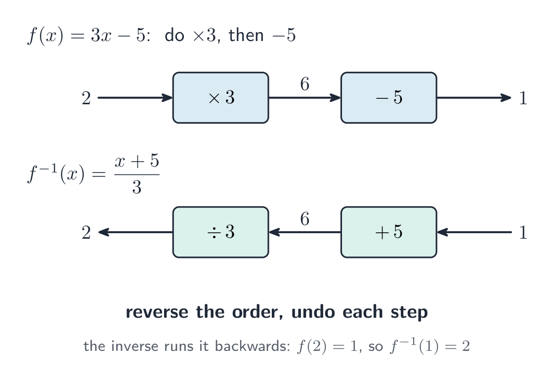
A function is invertible 可逆 on a domain where each output has exactly one input. Its inverse function 反函数 $f^{-1}$ reverses the mapping: if $f(a)=b$, then $f^{-1}(b)=a$. The notation $f^{-1}$ means inverse, not the reciprocal $1/f$.
- Domain and range 值域 swap. Reverse $(a,b)$ to $(b,a)$ in a table; reflect the graph across $y=x$ using equal axis units.
- Check both compositions on their proper domains: $f^{-1}(f(x))=x$ for inputs of $f$, and $f(f^{-1}(y))=y$ for inputs of $f^{-1}$.
- To find a formula, write $y=f(x)$, solve for $x$, then rename the inverse input. Retain the original domain and range while solving.
Worked example: select a branch. The function $x^2$ on all real inputs is not one-to-one, since $2$ and $-2$ both give 4. Restricting to $x\ge0$ gives inverse $\sqrt x$, while restricting to $x\le0$ gives inverse $-\sqrt x$; both inverse domains are $x\ge0$. Writing $\pm\sqrt x$ would not define a single-valued inverse function.
Worked example: a contextual inverse. If $T(t)=20+80(0.5)^t$ for $t\ge0$, its outputs are $20<T\le100$. Solving for elapsed time gives
$$\begin{aligned}
T-20&=80(0.5)^t,\\
t&=\frac{\ln((T-20)/80)}{\ln(0.5)}.
\end{aligned}$$
The contextual inverse accepts $20<T\le100$ and returns $t\ge0$. A temperature above 100 would give a negative time in the extended formula, outside this context; 20 is never reached at a finite time.
Try it. Find the inverse of $f(x)=3x-2$ on all real inputs, and verify one composition.
Check. $f^{-1}(x)=(x+2)/3$; $f^{-1}(f(x))=(3x-2+2)/3=x$. Both domains and ranges are all real numbers.
Worked example. Find the inverse of $f(x)=2e^{x}+1$. Write $x=2e^{y}+1$ and solve for $y$:
$$x-1=2e^{y} \;\Rightarrow\; e^{y}=\frac{x-1}{2} \;\Rightarrow\; y=\ln\!\left(\frac{x-1}{2}\right).$$
So $f^{-1}(x)=\ln\!\left(\dfrac{x-1}{2}\right)$, with domain $x>1$: the range of $f$ (it is always above its asymptote $y=1$) becomes the domain of $f^{-1}$.
Explore
Inverse pairs and restricted square branches
Reflect the chosen invertible domain across y=x and exchange domain with range.
Vocabulary
Train
| English |
|---|
| invertible/ɪnˈvɜːtɪbl/ |
| inverse function/ɪnˈvɜːs ˈfʌŋkʃn/ |
| range/reɪndʒ/ |
2.9
Logarithmic Expressions
Syllabus
| Learning Objective | Essential Knowledge |
|---|---|
2.9.A |
|
Source: College Board AP Course and Exam Description
The logarithm 对数 answers “what exponent?”: $\log_b c=a$ means $b^a=c$. Real logarithms require $b>0$, $b\ne1$ and $c>0$. The output can be positive, zero or negative: $\log_2 8=3$, $\log_2 1=0$ and $\log_2(1/8)=-3$.
An unwritten base in this chapter means the common logarithm 常用对数, base 10. The natural logarithm 自然对数 is $\ln x=\log_e x$, where $e\approx2.718$. State other bases explicitly: $\log_2 16=4$ differs from $\log_{10}16\approx1.204$.
A logarithmic scale 对数刻度 is a scale with equal spacing for equal factors. The values $1,10,100,1000$ are equally spaced on a base-10 scale. Its midpoint between 10 and 100 is $\sqrt{1000}\approx31.623$, not 55. Zero and negative values have no finite position on a standard real log scale.
Estimate before using technology. Since $2^3<12<2^4$, $3<\log_2 12<4$. With a base between zero and one, powers decrease: $(1/2)^2=1/4$ and $(1/2)^3=1/8$, so $2<\log_{1/2}(1/5)<3$.
Try it. Evaluate $\log_3(1/9)$ and $\log_5 1$. Is $\log_2(-4)$ a real number?
Check. The values are $-2$ and 0. The last expression has no real value because a positive-base exponential cannot output $-4$.
Explore
Logarithms and equal-ratio scales
Read a logarithm as an exponent, then compare equal multiplicative steps with equal additive steps.
Vocabulary
Train
| English |
|---|
| logarithm/ˈlɒɡərɪθəm/ |
| common logarithm/ˈkɒmən ˈlɒɡərɪθəm/ |
| natural logarithm/ˈnætʃərəl ˈlɒɡərɪθəm/ |
| logarithmic scale/ˌlɒɡəˈrɪθmɪk skeɪl/ |
2.10
Inverses of Exponential Functions

Syllabus
| Learning Objective | Essential Knowledge |
|---|---|
2.10.A |
|
Source: College Board AP Course and Exam Description
For $b>0$, $b\ne1$, the functions $y=b^x$ and $y=\log_b x$ undo each other. Their domains and ranges swap: the exponential accepts all real inputs and outputs positive values, while the logarithm accepts positive inputs and outputs all real values. In the identities below, the first allows every real input; the second requires $x>0$.
$$\begin{aligned}
\log_b(b^x)&=x,\\
b^{\log_b x}&=x.
\end{aligned}$$
Worked example: retain the scale factor. For $f(x)=2^x$, $f(3)=8$ gives $f^{-1}(8)=3$. For $F(x)=2\cdot2^x$, solving $y=2\cdot2^x$ gives $F^{-1}(y)=\log_2(y/2)$, not $2\log_2 y$. In particular, $F(3)=16$ and $F^{-1}(16)=3$.
Shifted inverse forms. For $F(x)=k+ab^{x-h}$ with $a\ne0$, isolate $(y-k)/a=b^{x-h}$:
$$F^{-1}(y)=h+\frac{\ln((y-k)/a)}{\ln b}.$$
The inverse needs $(y-k)/a>0$, the original function's range. It accepts $y>k$ when $a>0$ and $y<k$ when $a<0$. Its outputs are all real numbers unless the original input was restricted by context.
Try it. For $G(x)=3+2^x$, find $G^{-1}(x)$ and its domain.
Check. $G^{-1}(x)=\log_2(x-3)$, with $x>3$.
Explore
Matched exponential and logarithmic inverses
Reflect valid points and match the logarithmic scale factor with the exponential denominator.
2.11
Logarithmic Functions
Syllabus
| Learning Objective | Essential Knowledge |
|---|---|
2.11.A |
|
Source: College Board AP Course and Exam Description
The logarithmic function 对数函数 $f(x)=\log_b x$, with $b>0$, $b\ne1$, has domain $x>0$ and range all real numbers. It passes through $(1,0)$ and has a vertical asymptote at $x=0$.
- For $b>1$, it is increasing and concave down. As $x\to0^+$, $f(x)\to-\infty$; as $x\to\infty$, $f(x)\to\infty$.
- For $0<b<1$, it is decreasing and concave up. The two limits reverse: $f(x)\to\infty$ as $x\to0^+$ and $f(x)\to-\infty$ as $x\to\infty$.
There are no turning or inflection points. An unbounded function can still change slowly: an increasing logarithm does not have a horizontal ceiling. On a closed interval within its domain, the largest and smallest values occur at endpoints.
Read proportional inputs. Multiplying a positive input by $b$ adds 1 to its logarithm. For $H(x)=a\log_b(x-h)+k$, multiply the adjusted input $x-h$ by $b$ to add $a$ to the output. Equal ordinary input increments generally do not produce equal output increments.
Worked example: a reflected logarithm. For $H(x)=-2\log_2(x-3)+1$, the domain is $x>3$, the asymptote is $x=3$, and $H(4)=1$. A negative coefficient reverses the direction and concavity of the increasing base-2 logarithm: this function decreases and is concave up. Its values tend to $+\infty$ near $3^+$ and to $-\infty$ as $x\to\infty$.
Try it. Find the domain and value at $x=5$ of $K(x)=\log_{1/2}(x-1)$.
Check. The domain is $x>1$; $K(5)=\log_{1/2}4=-2$.
Explore
Direction, concavity and shifted logarithmic domains
Compare successive unit-input changes; use the base and nonzero scale factor together to identify shape and end behavior.
Vocabulary
Train
| English |
|---|
| logarithmic function/ˌlɒɡəˈrɪθmɪk ˈfʌŋkʃn/ |
2.12
Logarithmic Function Manipulation
Syllabus
| Learning Objective | Essential Knowledge |
|---|---|
2.12.A |
|
Source: College Board AP Course and Exam Description
For $b>0$, $b\ne1$, $x>0$ and $y>0$, the log laws are
$$\begin{aligned}
\log_b(xy)&=\log_b x+\log_b y,\\
\log_b(x/y)&=\log_b x-\log_b y,\\
\log_b(x^r)&=r\log_b x.
\end{aligned}$$
The positive-input conditions matter. For example, $\ln(x^2)=2\ln|x|$ for $x\ne0$; the form $2\ln x$ only covers $x>0$. Combining $\ln(x-1)+\ln(x+1)$ gives $\ln(x^2-1)$ with the original restriction $x>1$. The combined expression alone also exists for $x<-1$, which the original sum does not permit.
There is no corresponding sum law: $\log_b(x+y)$ is not generally $\log_b x+\log_b y$. At $x=y=1$, base 10 gives $\log_{10}2\ne0+0$.
The change-of-base 换底 formula uses any valid base $q$:
$$\begin{aligned}
\log_b x&=\frac{\log_q x}{\log_q b},\\
&=\frac{\ln x}{\ln b},\qquad x>0.
\end{aligned}$$
Changing a base rescales the output: $\log_{b^r}x=(1/r)\log_b x$ for $r\ne0$. Multiplying the input by $c>0$ instead shifts the output: $\log_b(cx)=\log_b x+\log_b c$.
Try it. Expand $\ln(x^2/y)$ for $x\ne0$, $y>0$, without losing the negative values of $x$.
Check. $\ln(x^2/y)=2\ln|x|-\ln y$, retaining $x\ne0$, $y>0$.
Explore
Logarithm identities with retained domains
Compare single and expanded logarithms, their domains and the graph transformations they represent.
Vocabulary
Train
| English |
|---|
| change-of-base/tʃeɪndʒ ɒv beɪs/ |
2.13
Exponential and Logarithmic Equations and Inequalities
Syllabus
| Learning Objective | Essential Knowledge |
|---|---|
2.13.A |
|
2.13.B |
|
Source: College Board AP Course and Exam Description
First state any input restrictions. Isolate an exponential before taking logs, or isolate a logarithm before exponentiating. Extraneous solutions 增根 are the candidate answers that fail the original relation or its domain conditions. Substitute candidates back into the original relation to reject them.
Worked example: an equation. Solve $2\cdot3^x=54$. Dividing by 2 gives $3^x=27=3^3$, so $x=3$. If powers are not tidy, $5^x=20$ gives $x=\ln20/\ln5\approx1.861$. A relation such as $2^x=-3$ has no real solution because its left side is positive.
Worked example: a rejected root. Solve $\ln(x-1)+\ln(x-2)=\ln2$. The original domain is $x>2$. Combining the logs gives
$$\begin{aligned}
(x-1)(x-2)&=2,\\
x^2-3x&=0,\\
x(x-3)&=0.
\end{aligned}$$
Candidates 0 and 3 satisfy the combined algebraic equation. Only $x=3$ lies in the original domain; $x=0$ makes both original log arguments negative.
Worked example: inequality direction and endpoints. For $\log_2(x-1)\ge2$, the domain is $x>1$. Base 2 is increasing, so $x-1\ge4$, giving $x\ge5$, including the endpoint. For $\log_{1/2}(x-1)\ge2$, the logarithm decreases, so $x-1\le1/4$. Intersecting with the domain gives $1<x\le5/4$: the domain boundary is excluded and the equality boundary is included.
Ordinary algebra can also reverse an inequality. For $-2\cdot3^x\ge-18$, dividing by $-2$ gives $3^x\le9$, hence $x\le2$. Keep this sign reversal separate from a reversal caused by a decreasing function.
Try it. Solve $\log_2(x-2)<1$ and $2^x\le0$. If a time equation gives $t=-1$, can it answer a question restricted to $t\ge0$?
Check. The first solution is $2<x<4$; the second has no real solutions. A negative time must be rejected in that stated context, even when it solves an extended mathematical equation.
Worked example: an extraneous solution. Solve $\log_2 x+\log_2(x-2)=3$. Combine with the product property, then exponentiate:
$$\log_2\big(x(x-2)\big)=3 \;\Rightarrow\; x(x-2)=2^3=8 \;\Rightarrow\; x^2-2x-8=0 \;\Rightarrow\; (x-4)(x+2)=0.$$
So $x=4$ or $x=-2$. Check each in the original equation: $x=-2$ makes $\log_2(-2)$ undefined, so reject it. The only solution is $x=4$ (check: $\log_2 4+\log_2 2=2+1=3$).
Explore
Boundaries and domains in solution sets
Read crossings and solution intervals, including decreasing bases, strict endpoints and nonpositive exponential targets.
Vocabulary
Train
| English |
|---|
| extraneous solutions |
2.14
Logarithmic Function Context and Data Modeling
Syllabus
| Learning Objective | Essential Knowledge |
|---|---|
2.14.A |
|
Source: College Board AP Course and Exam Description
A logarithmic model 对数模型 is a model whose output is linear in the logarithm of its input. A doubling process can be described in two directions. If $N(t)=100(2)^t$, amount is an exponential function of time. Solving for elapsed time instead gives a logarithmic model:
$$\begin{aligned}
T(N)&=\log_2(N/100),\\
&=\frac{\ln(N/100)}{\ln2}.
\end{aligned}$$
Here $T(100)=0$ and each doubling of the input amount adds one hour. The mathematical domain is $N>0$; a process starting at time zero uses $N\ge100$. At amount 300, the model predicts about 1.585 hours, assuming continuous growth between observations.
Worked example: two observations. Fix the unshifted form $y=a\log_{10}x+c$. Observations $(1,1)$ and $(10,3)$ give $c=1$, $a=2$, hence $y=2\log_{10}x+1$. For any fixed valid base, two distinct positive inputs give
$$\begin{aligned}
a&=\frac{y_2-y_1}{\log_b x_2-\log_b x_1},\\
c&=y_1-a\log_b x_1.
\end{aligned}$$
The parameters 参数 have specific meanings: $c$ is the model output at input 1, and multiplying the input by $b$ adds $a$ to the output. The logarithm is undefined at input zero. An unknown input shift adds another parameter and needs additional information.
Fit and check noisy data. A logarithmic regression 对数回归 is a least-squares fit of an output against a logarithm of its positive input. It does not log the output. For illustrative observations $(1,1.2)$, $(10,2.6)$ and $(100,5.2)$, the least-squares fit is $\hat y=2\log_{10}x+1$. Its residuals are $0.2,-0.4,0.2$, with squared sum 0.24. A regression can pass through some or all observations; fitting within this family does not prove that the family is appropriate.
Separate domain from support. Interpolation 内插 is a prediction at an input between the observed input limits. Extrapolation 外推 is a prediction beyond the observed input limits. With observations only at inputs 1 and 10, predicting at 5 interpolates, while predicting at 100 extrapolates. The formula gives about 2.398 at 5 and 5 at 100, but both predictions require modeling assumptions, especially beyond the observations. A score model $S(h)=20\log_{10}h+40$ can be a local fit; it cannot describe a score capped at 100 for every positive $h$, since $S(10000)=120$.
For a shifted example $P(t)=10\ln(t+1)+5$, the mathematical domain is $t>-1$, with $P(0)=5$ and $P(e-1)=15$. Proportional changes belong to the adjusted input $t+1$. Choose or estimate a shift for a contextual reason, not just to hide an invalid log argument.
Try it. For $y=3\log_{10}x+2$, find the output at 100 and the output change when a positive input is multiplied by 10. Does a decreasing curve that flattens always justify a logarithmic model?
Check. The output is 8 and the increment is 3. Shape alone is insufficient: an exponential decay or a bounded process can also flatten. Check which variable is the input, ratios, residuals and context.
Explore
Logarithmic construction, regression and prediction support
Fit observations, inspect residuals, and distinguish mathematical inputs from observed and extrapolated ranges.
Vocabulary
Train
| English |
|---|
| logarithmic model/ˌlɒɡəˈrɪθmɪk ˈmɒdl/ |
| parameters/pəˈræmɪtəz/ |
| logarithmic regression |
| interpolation/ɪnˌtɜːpəˈleɪʃn/ |
| extrapolation/ekˈstræpəleɪʃn/ |
2.15
Semi-log Plots
Syllabus
| Learning Objective | Essential Knowledge |
|---|---|
2.15.A |
|
2.15.B |
|
Source: College Board AP Course and Exam Description
A semi-log plot 半对数图 has exactly one logarithmic axis. With a linear horizontal axis and a logarithmic vertical axis, a positive exponential $y=ab^x$ gives a straight pattern:
$$\begin{aligned}
z=\log_q y&=mx+c,\\
m&=\log_q b,\\
c&=\log_q a,\\
a&=q^c,\\
b&=q^m.
\end{aligned}$$
Here $a>0$, $b>0$ and the scale base $q>1$. The transformed slope 斜率 describes log change per input unit. The intercept 截距 is the log of the original initial value, not that value itself. A log-scaled axis can label ticks with the original $y$ values; an ordinary axis labelled $z=\log_q y$ instead displays their logged coordinates. Do not log a value twice.
Worked example: recover a model. Observations $(0,100)$ and $(4,10000)$ become $(0,2)$ and $(4,4)$ when base-10 outputs are logged. Then $m=(4-2)/4=0.5$, $c=2$, so $y=100\cdot10^{0.5x}$. At $x=2$, the output is 1000. The per-unit factor is $10^{0.5}$, not 0.5.
Growth and decay. For $q>1$, a positive slope means growth, a negative slope means decay, and zero slope gives a positive constant. If $\log_{10}y=2-0.25t$, the initial amount is 100 and the factor per time unit is $10^{-0.25}\approx0.5623$, a decrease of about $43.77\%$. Half the initial amount is reached at $t=\log_{10}2/0.25\approx1.204$ time units.
Changing the log base changes the numerical slope, not the original model. For $y=4(2)^x$ with $x$ in hours, the base-2 line is $z=x+2$; base 10 gives slope $\log_{10}2$ and intercept $\log_{10}4$. With time in minutes, the base-2 slope becomes $1/60$ per minute. Compare slopes only with a common base and input units.
Read the orientation. If the horizontal axis is logarithmic and the vertical axis is linear, a logarithmic form $y=a\log_q x+c$ gives a line instead. A standard real log axis excludes nonpositive values. With both axes logarithmic, the graph is not semi-log.
Use evidence carefully. Two transformed points always determine a line if their inputs differ; they do not establish a reliable exponential model. Noisy exponential observations may deviate from a line. Fitting a line to $\log y$ minimises log errors rather than errors in the original output, so it is not automatically more accurate for the intended prediction. A vertical offset such as $y=4(2)^x+4$ generally prevents a straight log-output pattern; subtract a baseline only when justified.
Try it. For $y=4(2)^x$, find the original output and its base-2 log coordinate at $x=3$. Can a positive constant also give a straight semi-log pattern?
Check. The original output is 32 and its transformed coordinate is 5. The axis labels distinguish them. A positive constant gives a horizontal straight line, with factor 1 and transformed slope zero.
Worked example. On a semi-log plot (base $10$), data lie on the line $\log y=0.301+0.477x$. Undo each logarithm: $a=10^{0.301}\approx 2$ and $b=10^{0.477}\approx 3$, so the model is $y\approx 2\cdot 3^x$. A slope of $0.477$ means $y$ is multiplied by $10^{0.477}\approx3$ for every increase of $1$ in $x$.
Explore
Ordinary and logarithmic vertical scales
Compare the same outputs and recover factors from transformed slopes.
Vocabulary
Train
| English |
|---|
| semi-log plot/ˈsemi lɒɡ plɒt/ |
| slope/sləʊp/ |
| intercept/ˌɪntəˈsept/ |
2.15
Exam tips
- State domains and input units; compare differences or ratios over equal input intervals.
- Track the input/output order in composition, and preserve restrictions after simplifying. An inverse reverses a one-to-one mapping on its stated domain.
- Check signs, bases, shifts and contextual restrictions. Negative coefficients and bases below 1 can reverse direction in different ways.
- Use logarithm laws only where their arguments are valid; keep absolute values when needed and reject extraneous roots in the original relation.
- Distinguish a fitted model from a reliable prediction. Inspect residuals and the observed range before extrapolating.
- On semi-log axes, identify which axis is logarithmic, the scale base and the input unit before interpreting a straight line or its slope.
Cumulative checkpoint
- Let $H(x)=\sqrt{2x-4}$. State its domain, then find the inverse and the inverse's domain.
- Solve $\ln(x-1)+\ln(x+1)=\ln8$. State the original domain before combining logs.
- Solve $\log_{1/2}(x-1)>-1$. Explain both endpoints of the solution interval.
- A base-10 semi-log model is $\log_{10}y=0.2t+1$, with $t$ in hours. Recover the initial value, hourly factor and prediction at hour 5. If observations cover hours 0–5, classify a prediction at hour 6.
Answers and reasoning.
- $H$ needs $2x-4\ge0$, so $x\ge2$, and has range $y\ge0$. Solving $y^2=2x-4$ gives $H^{-1}(x)=(x^2+4)/2$ for $x\ge0$. Its domain is the original range, not all real inputs.
- The original domain is $x>1$. Combining gives $x^2-1=8$, hence candidates $x=\pm3$. Only $x=3$ is allowed.
- The log argument requires $x>1$. The decreasing base reverses the inequality, giving $x-1<2$, so $1<x<3$. Input 1 is undefined and input 3 gives equality, which the strict inequality excludes.
- $y=10(10^{0.2})^t$: initial value 10, hourly factor $10^{0.2}\approx1.585$, and $y(5)=10(10)=100$. Hour 6 is extrapolation and needs further justification.
Interactive lessons on this topic
Work through it step by step, with instant-check exercises.
- Arithmetic and Geometric Sequences
- Linear and Exponential Functions
- Exponential Functions
- Manipulating Exponential Expressions
- Modeling with Exponential Functions
- Comparing Competing Models
- Composition of Functions
- Inverse Functions
- Logarithms
- Inverses of Exponential Functions
- Logarithmic Functions
- Manipulating Logarithmic Expressions
- Exponential and Logarithmic Equations and Inequalities
- Modeling with Logarithmic Functions
- Semi-log Plots