Skip to content · ⁨דלג לתוכן⁩

Exponential and Logarithmic Functions · ⁨פונקציות מעריכיות ולוגריתמיות⁩

AP Precalculus · ⁨פרי-קלקולוס - AP⁩ · Topic 2 · ⁨נושא 2⁩

Video lesson for this topic · ⁨שיעור וידאו לנושא זה⁩ Open the video page · ⁨פתח את עמוד הוידאו⁩
14:05

פונקציות מעריכיות ולוגריתמיות

הנה שתי דרכים לצמיחה של כמות. הקו הכחול צומח באופן רציף, מוסיף את אותו סכום בכל צעד. האחרת היא הכפל – מכפילים ב…

English narration · English + 中文 subtitles burned in · ⁨קריאת קול באנגלית · תרגום אנגלי + סינית שרוף בתוך הסרטון⁩

2.1

Change in Arithmetic and Geometric Sequences · ⁨שינוי בסדרות אריתמטיות וגיאומטריות⁩

Syllabus · ⁨סיילבוס⁩
English

Learning Objective 2.1.A: Express arithmetic sequences found in mathematical and contextual scenarios as functions of the whole numbers.

  • 2.1.A.1 A sequence is a function from the whole numbers to the real numbers. Consequently, the graph of a sequence consists of discrete points instead of a curve.
  • 2.1.A.2 Successive terms in an arithmetic sequence have a common difference, or constant rate of change.
  • 2.1.A.3 The general term of an arithmetic sequence with a common difference $d$ is denoted by $a_n$ and is given by $a_n = a_0 + dn$, where $a_0$ is the initial value, or by $a_n = a_k + d(n - k)$, where $a_k$ is the $k$th term of the sequence.

Learning Objective 2.1.B: Express geometric sequences found in mathematical and contextual scenarios as functions of the whole numbers.

  • 2.1.B.1 Successive terms in a geometric sequence have a common ratio, or constant proportional change.
  • 2.1.B.2 The general term of a geometric sequence with a common ratio $r$ is denoted by $g_n$ and is given by $g_n = g_0 r^n$, where $g_0$ is the initial value, or by $g_n = g_k r^{(n-k)}$, where $g_k$ is the $k$th term of the sequence.
  • 2.1.B.3 Increasing arithmetic sequences increase equally with each step, whereas increasing geometric sequences increase by a larger amount with each successive step.
עברית

מטרות למידה 2.1.A: ביטוי סדרות חשוניות הנמצאות בתרחישים מתמטיים ובתרחישים קונטקסטואליים כפונקציות של המספרים השלמים.

  • 2.1.A.1 סדרה היא פונקציה מהמספרים השלמים אל המספרים הממשיים. כתוצאה מכך, הגרף של סדרה מורכב מנקודות בדידות ולא מעקומה.
  • 2.1.A.2 איברים עוקבים בסדרה חשונית בעלי הפרש משותף, או קצב שינוי קבוע.
  • 2.1.A.3 האיבר הכללי של סדרה חשונית עם הפרש משותף $d$ מסומן על ידי $a_n$ ונתון על ידי $a_n = a_0 + dn$, כאשר $a_0$ הוא הערך ההתחלתי, או על ידי $a_n = a_k + d(n - k)$, כאשר $a_k$ הוא האיבר ה$k$ בסדרה.

מטרות למידה 2.1.B: ביטוי סדרות גיאומטריות הנמצאות בתרחישים מתמטיים ובתרחישים קונטקסטואליים כפונקציות של המספרים השלמים.

  • 2.1.B.1 איברים עוקבים בסדרה גיאומטרית בעלי יחס משותף, או שינוי פרופורציונלי קבוע.
  • 2.1.B.2 האיבר הכללי של סדרה גיאומטרית עם יחס משותף $r$ מסומן על ידי $g_n$ ונתון על ידי $g_n = g_0 r^n$, כאשר $g_0$ הוא הערך ההתחלתי, או על ידי $g_n = g_k r^{(n-k)}$, כאשר $g_k$ הוא האיבר ה$k$ בסדרה.
  • 2.1.B.3 סדרות חשוניות עולות גדלות באופן שווה בכל צעד, בעוד שסדרות גיאומטריות עולות גדלות בכמות גדולה יותר בכל צעד עוקב.

Source: College Board AP Course and Exam Description · ⁨מקור: תיאור הקורס והמבחן של College Board AP⁩

English
Geometric series & convergence

A sequence 数列 is a function from the whole numbers to the real numbers, so its graph is discrete points, not a curve.

  • An arithmetic sequence 等差数列 has a common difference 公差 $d$ (a constant rate of change): $a_n = a_0 + dn$, or from a known term, $a_n = a_k + d(n-k)$.
  • A geometric sequence 等比数列 has a common ratio 公比 $r$ (a constant proportional change): $g_n = g_0\,r^{\,n}$, or $g_n = g_k\,r^{\,(n-k)}$.

An increasing arithmetic sequence grows by the same amount each step; an increasing geometric sequence grows by a larger amount each step.

Worked example. An arithmetic sequence with $a_0=3$ and $d=5$ has $a_4=3+5(4)=23$. A geometric sequence with $g_0=2$ and $r=3$ has $g_4=2\cdot3^4=162$ – addition versus multiplication makes the geometric one pull far ahead.

עברית
סדרה גיאומטרית & התכנסות

סדרה היא פונקציה מהמספרים הטבעיים למספרים הממשיים, ולכן הגרף שלה הוא נקודות בדידות, לא עקומה.

סדרה אריתמטית עולה בשלבים שווים; סדרה גיאומטרית מכפילה ביחס
סדרה אריתמטית עולה בשלבים שווים; גיאומטרית כופלת ביחס
  • סדרה אריתמטית יש לההפרש משותף $d$ (קצב שינוי קבוע): $a_n = a_0 + dn$, או מאיבר ידוע, $a_n = a_k + d(n-k)$.
  • סדרה גיאומטרית יש להיחס משותף $r$ (שינוי פרופורציונלי קבוע): $g_n = g_0\,r^{\,n}$, או $g_n = g_k\,r^{\,(n-k)}$.

סדרה חשוכית עולה גדלה ב-אותו כמות בכל צעד; סדרה גיאומטרית עולה גדלה בכמות גדולה יותר בכל צעד.

דוגמה מפורטת. סדרה חשוכית עם $a_0=3$ ו$d=5$ היא $a_4=3+5(4)=23$. סדרה גיאומטרית עם $g_0=2$ ו$r=3$ היא $g_4=2\cdot3^4=162$ – ההבדל בין חיבור לכפל גורם לכך שהסדרה הגיאומטרית תופסת רחוק.

Explore · ⁨חקור⁩

Compare arithmetic and geometric growth · ⁨השווה בין גידול אריטמטי לגיאומטרי⁩

An arithmetic sequence adds a fixed step each term (linear); a geometric sequence multiplies by a fixed ratio (exponential). Change the ratio and watch the terms explode or decay. · ⁨סדרה אריטמטית מוסיפה שלב קבוע בכל איבר (ליניאר); סדרה גיאומטרית מכפילה ביחס קבוע (אקספוננציאלי). שנה את היחס וצפה באיברים מתפוצצים או מדעכים.⁩

2.2

Change in Linear and Exponential Functions · ⁨שינוי בפונקציות ליניאריות ואקספוננציאליות⁩

Syllabus · ⁨סיילבוס⁩
English

Learning Objective 2.2.A: Construct functions of the real numbers that are comparable to arithmetic and geometric sequences.

  • 2.2.A.1 Linear functions of the form $f(x) = b + mx$ are similar to arithmetic sequences of the form $a_n = a_0 + dn$, as both can be expressed as an initial value ($b$ or $a_0$) plus repeated addition of a constant rate of change, the slope ($m$ or $d$).
  • 2.2.A.2 Similar to arithmetic sequences of the form $a_n = a_k + d(n - k)$, which are based on a known difference, $d$, and a $k$th term, linear functions can be expressed in the form $f(x) = y_i + m(x - x_i)$ based on a known slope, $m$, and a point, $(x_i, y_i)$.
  • 2.2.A.3 Exponential functions of the form $f(x) = ab^x$ are similar to geometric sequences of the form $g_n = g_0 r^n$, as both can be expressed as an initial value ($a$ or $g_0$) times repeated multiplication by a constant proportion ($b$ or $r$).
  • 2.2.A.4 Similar to geometric sequences of the form $g_n = g_k r^{(n-k)}$, which are based on a known ratio, $r$, and a $k$th term, exponential functions can be expressed in the form $f(x) = y_i r^{(x - x_i)}$ based on a known ratio, $r$, and a point, $(x_i, y_i)$.
  • 2.2.A.5 Sequences and their corresponding functions may have different domains.
עברית

מטרות לימוד 2.2.A: בניית פונקציות של המספרים הממשיים השוות לסידורים אריתמטיים וגיאומטריים.

  • 2.2.A.1 פונקציות ליניאריות בצורת $f(x) = b + mx$ דומות לסדרות אריתמטיות בצורת $a_n = a_0 + dn$, שכן שתיהן ניתנות לביטוי כערך התחלתי ($b$ או $a_0$) פלוס חיבור חוזר של קצב שינוי קבוע, השיפוע ($m$ או $d$).
  • 2.2.A.2 בדומה לסדרות אריתמטיות בצורה $a_n = a_k + d(n - k)$, המבוססות על הפרש ידוע, $d$, ומונה $k$, פונקציות ליניאריות ניתן לבטא בצורה $f(x) = y_i + m(x - x_i)$ המבוססת על שיפוע ידוע, $m$, ונקודה, $(x_i, y_i)$.
  • 2.2.A.3 פונקציות אקספוננציאליות בצורת $f(x) = ab^x$ דומות לסדרות גיאומטריות בצורת $g_n = g_0 r^n$, שכן שתיהן ניתנות לביטוי כערך התחלתי ($a$ או $g_0$) כפול כפל חוזר של פרופורציה קבועה ($b$ או $r$).
  • 2.2.A.4 כפי שסדרות גיאומטריות של צורה $g_n = g_k r^{(n-k)}$, המבוססות על יחס ידוע, $r$, ומונע $k$-י, פונקציות מעריכיות יכולות להיות מיוצגות בצורה $f(x) = y_i r^{(x - x_i)}$ המבוססת על יחס ידוע, $r$, ונקודה, $(x_i, y_i)$.
  • 2.2.A.5 לסדרות ולפונקציות המתאימות להן עשויה להיות תחום הגדרה שונה.

Source: College Board AP Course and Exam Description · ⁨מקור: תיאור הקורס והמבחן של College Board AP⁩

English

Sequences have continuous cousins:

  • Linear functions $f(x)=b+mx$ mirror arithmetic sequences – an initial value plus repeated addition of the slope $m$. Point form: $f(x)=y_i+m(x-x_i)$.
  • Exponential functions $f(x)=ab^x$ mirror geometric sequences – an initial value times repeated multiplication by the base $b$. Point form: $f(x)=y_i\,r^{\,(x-x_i)}$.

The difference: linear = repeated addition, exponential = repeated multiplication. (A sequence and its function may have different domains.)

עברית
רוץ: מודלים אקספוננציאליים ולוגריתמיים מתארים קצבי גידול ודעיכה בהקשר

לסדרות יש בני דודים רציפים:

  • פונקציות ליניאריות $f(x)=b+mx$ משקפות סדרות חשוכיות – ערך התחלתי פלוס חיבור חוזר של השיפוע $m$. צורת נקודה: $f(x)=y_i+m(x-x_i)$.
  • פונקציות אקספוננציאליות $f(x)=ab^x$ משקפות סדרות גיאומטריות – ערך התחלתי כפול בחזרה כפילה על ידי הבסיס $b$. צורת נקודה: $f(x)=y_i\,r^{\,(x-x_i)}$.

ההבדל: ליניאר = חיבור חוזר, אקספוננציאלי = כפל חוזר. (לסדרה ולפונקציה עשויה להיות תחום הגדרה שונה.)

2.3

Exponential Functions · ⁨פונקציות אקספוננציאליות⁩

Syllabus · ⁨סיילבוס⁩
English

Learning Objective 2.3.A: Identify key characteristics of exponential functions.

  • 2.3.A.1 The general form of an exponential function is $f(x) = ab^x$, with the initial value $a$, where $a \neq 0$, and the base $b$, where $b > 0$, and $b \neq 1$. When $a > 0$ and $b > 1$, the exponential function is said to demonstrate exponential growth. When $a > 0$ and $0 < b < 1$, the exponential function is said to demonstrate exponential decay.
  • 2.3.A.2 When the natural numbers are input values in an exponential function, the input value specifies the number of factors of the base to be applied to the function's initial value. The domain of an exponential function is all real numbers.
  • 2.3.A.3 Because the output values of exponential functions in general form are proportional over equal-length input-value intervals, exponential functions are always increasing or always decreasing, and their graphs are always concave up or always concave down. Consequently, exponential functions do not have extrema except on a closed interval, and their graphs do not have points of inflection.
  • 2.3.A.4 If the values of the additive transformation function $g(x) = f(x) + k$ of any function $f$ are proportional over equal-length input-value intervals, then $f$ is exponential.
עברית

מטרת הלמידה 2.3.A: זיהוי מאפיינים מרכזיים של פונקציות מעריכיות.

  • 2.3.A.1 הצורה הכללית של פונקציה מעריכית היא $f(x) = ab^x$, עם הערך ההתחלתי $a$, כאשר $a \neq 0$, והבסיס $b$, כאשר $b > 0$, ו$b \neq 1$. כאשר $a > 0$ ו$b > 1$, הפונקציה המעריכית נחשבת המדגימה צמיחה מעריכית. כאשר $a > 0$ ו$0 < b < 1$, הפונקציה המעריכית נחשבת המדגימה דעיכה מעריכית.
  • 2.3.A.2 כאשר המספרים הטבעיים הם ערכי הקלט בפונקציה מעריכית, ערך הקלט קובע את מספר הגורמים מבסיס שהושתקו בערך ההתחלתי של הפונקציה. תחום ההגדרה של פונקציה מעריכית הוא כל המספרים הממשיים.
  • 2.3.A.3 מכיוון שערכי הפלט של פונקציות מעריכיות בצורה הכללית פרופורציונליים על פני רווחי ערכי קלט בעלי אורך שווה, פונקציות מעריכיות תמיד עולות או תמיד יורדות, וגרפים שלהן תמיד קעורים כלפי מעלה או תמיד קעורים כלפי מטה. כתוצאה מכך, לפונקציות מעריכיות אין מקסים מינימלי/מקסימום מוחלט מלבד ברווח סגור, וגרפים שלהן אינם מכילים נקודות היפוך.
  • 2.3.A.4 אם ערכי פונקציית ההמרה האדיטיבית $g(x) = f(x) + k$ של כל פונקציה $f$ הם פרופורציונליים על פני מרווחי ערכי קלט בעלי אורך שווה, אזי $f$ הוא מעריכי.

Source: College Board AP Course and Exam Description · ⁨מקור: תיאור הקורס והמבחן של College Board AP⁩

English

The general exponential function 指数函数 is $f(x)=ab^x$ with initial value 初始值 $a\neq 0$ and base 底数 $b>0,\ b\neq 1$. Domain: all real numbers.

  • $a>0,\ b>1$ gives exponential growth 指数增长; $a>0,\ 0 gives exponential decay 指数衰减.
  • Outputs are proportional over equal-length input intervals. So an exponential is always increasing or always decreasing, and always concave up or always concave down – it has no extrema (except on a closed interval) and no points of inflection.
עברית

הפונקציה האקספוננציאלית הכללית היא $f(x)=ab^x$ עם ערך התחלתי $a\neq 0$ ובסיס $b>0,\ b\neq 1$. תחום הגדרה: כל המספרים הממשיים.

דעיכה אקספוננציאלית: אחוז קבוע מאבד בכל תקופה
  • $a>0,\ b>1$ נותן גידול אקספוננציאלי; $a>0,\ 0 נותן דעיכה אקספוננציאלית.
  • הערכים היוצאים יחסיים לאורך רווחי קלט בעלי אותו אורך. לכן פונקציה אקספוננציאלית תמיד עולה או תמיד יורדת, ותמיד קעורה למעלה או תמיד קעורה למטה – אין לה נקודות קיצון (אלא בתחום סגור) ולא נקודות עיקול.
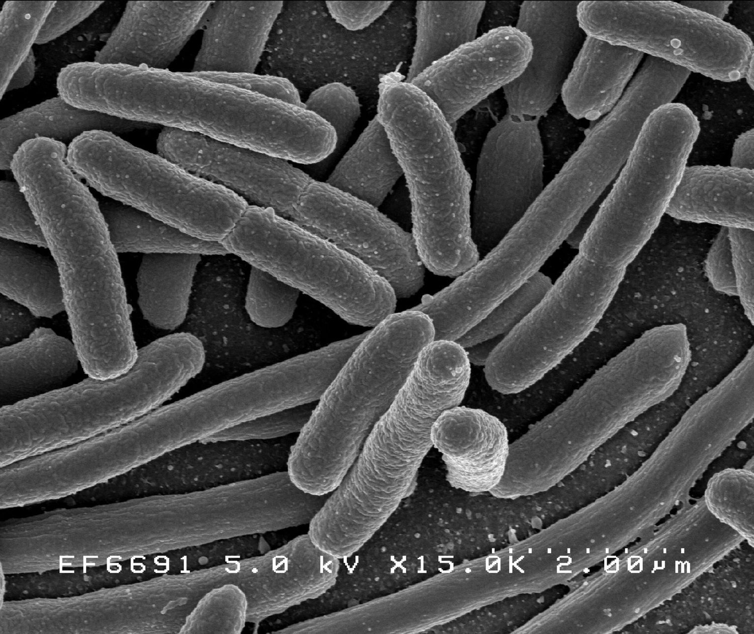
חיידקים תחת מיקרוסקופ: דגמים אקספוננציאליים מתארים אוכלוסיות הגדלות בפקטור קבוע בכל שלב זמן
בקטריות תחת מיקרוסקופ: מודלים אקספוננציאליים מתארים אוכלוסיות שגודלות בגורם קבוע בכל צעד זמן
Explore · ⁨חקור⁩

Explore an exponential curve · ⁨חקור עקום אקספוננציאלי⁩

y = a·e^(bx) + c

An exponential function changes by a constant factor over equal steps, so it rises (or decays) ever faster. The constant $c$ sets the horizontal asymptote it hugs. · ⁨פונקציה אקספוננציאלית משתנה על ידי גורם קבוע בשלבים שווים, ולכן היא עולה (או דועכת) בקצב תמיד גדל יותר. הקבוע $c$ קובע את האסימפטורה האופקית שהיא חובה.⁩

Vocabulary · ⁨מילון מונחים⁩ Train · ⁨אימון⁩
English עברית
sequence/ˈsiːkwəns/ רצף
arithmetic sequence/əˈrɪθmətɪk ˈsiːkwəns/ סדרה אריתמטית
common difference/ˈkɒmən ˈdɪfrəns/ הפרש שווה
geometric sequence/ˌdʒiːəʊˈmetrɪk ˈsiːkwəns/ סדרה גיאומטרית
common ratio/ˈkɒmən ˈreɪʃɪəʊ/ יחס דומה
exponential function/ˌekspəˈnenʃl ˈfʌŋkʃn/ פונקציה מעריכית
initial value/ɪˈnɪʃl ˈvæljuː/ ערך התחלתי⟦number⟧
base/beɪs/ בסיס
exponential growth/ˌekspəˈnenʃl ɡrəʊθ/ צמיחה מעריכית
exponential decay/ˌekspəˈnenʃl dɪˈkeɪ/ דעיכת מעריכית
root/ruːt/ שורש
exponential regression/ˌekspəˈnenʃl rɪˈɡreʃn/ רגרסיה אקספוננציאלית⟦number⟧
natural base/ˈnætʃərəl beɪs/ בסיס טבעי
residual plot/rɪˈsɪdʒuːəl plɒt/ גרף שאריות
residual/rɪˈsɪdʒuːəl/ שארית
composite function/ˈkɒmpəzɪt ˈfʌŋkʃn/ פונקציה מורכבת
identity function/aɪˈdentɪti ˈfʌŋkʃn/ פונקציית זהות
invertible/ɪnˈvɜːtɪbl/ הפיכה
2.4

Exponential Function Manipulation · ⁨עיבוד פונקציות אקספוננציאליות⁩

Syllabus · ⁨סיילבוס⁩
English

Learning Objective 2.4.A: Rewrite exponential expressions in equivalent forms.

  • 2.4.A.1 The product property for exponents states that $b^m b^n = b^{(m+n)}$. Graphically, this property implies that every horizontal translation of an exponential function, $f(x) = b^{(x+k)}$, is equivalent to a vertical dilation, $f(x) = b^{(x+k)} = b^x b^k = ab^x$, where $a = b^k$.
  • 2.4.A.2 The power property for exponents states that $\left(b^m\right)^n = b^{(mn)}$. Graphically, this property implies that every horizontal dilation of an exponential function, $f(x) = b^{(cx)}$, is equivalent to a change of the base of an exponential function, $f(x) = \left(b^c\right)^x$, where $b^c$ is a constant and $c \neq 0$.
  • 2.4.A.3 The negative exponent property states that $b^{-n} = \dfrac{1}{b^n}$.
  • 2.4.A.4 The value of an exponential expression involving an exponential unit fraction, such as $b^{(1/k)}$ where $k$ is a natural number, is the $k$th root of $b$, when it exists.
עברית

**מטרת הלמידה 2.4.A:**改写 פונקציות מעריכיות לצורות שקולות.

  • 2.4.A.1 תכונת הכפלה למעריכים קובעת כי $b^m b^n = b^{(m+n)}$. גרפית, תכונה זו מצביעה על כך שכל הזזת אופקית של פונקציה מעריכית, $f(x) = b^{(x+k)}$, שקולה להרחבה אנכית, $f(x) = b^{(x+k)} = b^x b^k = ab^x$, כאשר $a = b^k$.
  • 2.4.A.2 תכונת החזקה למעריכים קובעת כי $\left(b^m\right)^n = b^{(mn)}$. גרפית, תכונה זו מצביעה על כך שכל הרחבה אופקית של פונקציה מעריכית, $f(x) = b^{(cx)}$, שקולה לשינוי בבסיס של פונקציה מעריכית, $f(x) = \left(b^c\right)^x$, כאשר $b^c$ הוא קבוע ו$c \neq 0$.
  • 2.4.A.3 תכונת המעריך השלילי קובעת כי $b^{-n} = \dfrac{1}{b^n}$.
  • 2.4.A.4 הערך של ביטוי מעריכי המכיל שבר יחיד מעריכי, כמו $b^{(1/k)}$ כאשר $k$ הוא מספר טבעי, הוא השורש ה$k$-י של $b$, כאשר הוא קיים.

Source: College Board AP Course and Exam Description · ⁨מקור: תיאור הקורס והמבחן של College Board AP⁩

English

The exponent rules reshape exponential expressions and connect to graph transformations:

  • Product: $b^m b^n = b^{m+n}$. A horizontal shift $b^{x+k}$ equals a vertical stretch $ab^x$ with $a=b^k$.
  • Power: $(b^m)^n = b^{mn}$. A horizontal stretch $b^{cx}$ equals a base change $(b^c)^x$.
  • Negative exponent: $b^{-n}=\dfrac{1}{b^n}$.
  • Unit-fraction exponent: $b^{1/k}=\sqrt[k]{b}$ (the $k$th root 方根).
עברית

חוקי החזקות מעצבים ביטויים אקספוננציאליים ומקשרים להמרות גרף:

  • מכפלה: $b^m b^n = b^{m+n}$. הזזה אופקית $b^{x+k}$ שווה למתיחה אנכית $ab^x$ עם $a=b^k$.
  • חזקה: $(b^m)^n = b^{mn}$. מתיחה אופקית $b^{cx}$ שווה לשינוי בסיס $(b^c)^x$.
  • מעריך שלילי: $b^{-n}=\dfrac{1}{b^n}$.
  • מעריך כשבר יחיד: $b^{1/k}=\sqrt[k]{b}$ (השורש ה$k$).
2.5

Exponential Function Context and Data Modeling · ⁨הקשר פונקציה מעריכה ודגום נתונים⁩

Syllabus · ⁨סיילבוס⁩
English

Learning Objective 2.5.A: Construct a model for situations involving proportional output values over equal-length input-value intervals.

  • 2.5.A.1 Exponential functions model growth patterns where successive output values over equal-length input-value intervals are proportional. When the input values are whole numbers, exponential functions model situations of repeated multiplication of a constant to an initial value.
  • 2.5.A.2 A constant may need to be added to the dependent variable values of a data set to reveal a proportional growth pattern.
  • 2.5.A.3 An exponential function model can be constructed from an appropriate ratio and initial value or from two input-output pairs. The initial value and the base can be found by solving a system of equations resulting from the two input-output pairs.
  • 2.5.A.4 Exponential function models can be constructed by applying transformations to $f(x) = ab^x$ based on characteristics of a contextual scenario or data set.
  • 2.5.A.5 Exponential function models can be constructed for a data set with technology using exponential regressions.
  • 2.5.A.6 The natural base $e$, which is approximately $2.718$, is often used as the base in exponential functions that model contextual scenarios.
עברית

מטרת הלמידה 2.5.A: בניית מודל למצבים המכילים ערכי פלט פרופורציונליים על פני רווחי ערכי קלט בעלי אורך שווה.

  • 2.5.A.1 פונקציות מעריכיות מדגשות דפוסי גידול שבהם ערכי פלט רצופים על פני רווחי ערכי קלט בעלי אורך שווה הם פרופורציונליים. כאשר ערכי הקלט הם מספרים שלמים, פונקציות מעריכיות מדגשות מצבים של הכפלה חוזרת של קבוע לערך התחלתי.
  • 2.5.A.2 ייתכן שיש להוסיף קבוע לערכי משתנה התלוי במ数据集 כדי לחשוף דפוס גידול פרופורציונלי.
  • 2.5.A.3 ניתן לבנות מודל פונקציה מעריכית מתוך יחס מתאים וערך התחלתי, או מתוך שני זוגות קלט-פלט. את הערך ההתחלתי והבסיס ניתן למצוא על ידי פתרון מערכת משוואות הנובעת משני זוגות הקלט-פלט.
  • 2.5.A.4 ניתן לבנות מודלים לפונקציות מעריכיות על ידי יישום טרנספורמציות ל $f(x) = ab^x$ בהתבסס על מאפיינים של תרחיש רלוונטי או ערכי נתונים.
  • 2.5.A.5 ניתן לבנות מודלים לפונקציות מעריכיות עבור סט נתונים באמצעות טכנולוגיה, על בסיס רגרסיה מעריכית.
  • 2.5.A.6 הבסיס הטבעי $e$, השווה בקירוב ל $2.718$, משמש לעיתים קרובות כבסיס בפונקציות מעריכיות המדגמות תרחישים רלוונטיים.

Source: College Board AP Course and Exam Description · ⁨מקור: תיאור הקורס והמבחן של College Board AP⁩

English

Exponentials model quantities that grow by a constant proportion over equal intervals (repeated multiplication).

  • Build a model from a ratio and an initial value, or from two points (solve the system for $a$ and $b$).
  • Sometimes a constant must be added to the data to reveal the proportional pattern.
  • Use exponential regression 指数回归 on technology to fit a data set.
  • The natural base 自然底数 $e\approx 2.718$ is the standard base for real-world models.
עברית

פונקציות מעריכות מדגמות כמויות הגודלות ביחס קבוע על פני מרווחים שווים (כפל חוזר).

  • לבנות דגם מתוך יחס וערך התחלתי, או מתוך שתי נקודות (פתרון המערכת עבור $a$ ו$b$).
  • לעיתים יש להוסיף קבוע לנתונים כדי לחשוף את הדפוס היחסי.
  • השתמש ברגרסיה מעריכה בתוכנה כדי להתאים סט נתונים.
  • הבסיס הטבעי $e\approx 2.718$ הוא הבסיס הסטנדרטי לדגמים בעולם האמיתי.
2.6

Competing Function Model Validation · ⁨אימות דגם פונקציות מתחרות⁩

Syllabus · ⁨סיילבוס⁩
English

Learning Objective 2.6.A: Construct linear, quadratic, and exponential models based on a data set.

  • 2.6.A.1 Two variables in a data set that demonstrate a slightly changing rate of change can be modeled by linear, quadratic, and exponential function models.
  • 2.6.A.2 Models can be compared based on contextual clues and applicability to determine which model is most appropriate.

Learning Objective 2.6.B: Validate a model constructed from a data set.

  • 2.6.B.1 A model is justified as appropriate for a data set if the graph of the residuals of a regression, the residual plot, appear without pattern.
  • 2.6.B.2 The difference between the predicted and actual values is the error in the model. Depending on the data set and context, it may be more appropriate to have an underestimate or overestimate for any given interval.
עברית

מטרות לימוד 2.6.A: בניית מודלים ליניאריים, ריבועיים ומעריכיים על בסיס סט נתונים.

  • 2.6.A.1 שני משתנים בסט נתונים המציגים קצב שינוי משתנה מעט יכולים להיות מדומים על ידי מודלים לפונקציות ליניאריות, ריבועיות ומעריכיות.
  • 2.6.A.2 ניתן להשוות בין מודלים בהתבסס על רמזים מהתרחיש הרלוונטי וביצועיות כדי לקבוע איזה מודל הוא המתאים ביותר.

מטרות לימוד 2.6.B: אימות מודל שנבנה מסט נתונים.

  • 2.6.B.1 מודל נחשב מתאים לסט נתונים אם גרף שאריות הרגרסיה, כלומר גרף האשריות, מוצג ללא דפוס.
  • 2.6.B.2 ההפרש בין הערכים המנובאים לערכים האמיתיים הוא השגיאה במודל. בהתבסס על סט הנתונים והתרחיש, עשוי להיות יותר מתאים להשיג הערכת חיסרון או הערכת יתר לכל מרווח נתון.

Source: College Board AP Course and Exam Description · ⁨מקור: תיאור הקורס והמבחן של College Board AP⁩

English

When a rate of change shifts only slightly, linear, quadratic, and exponential models may all seem to fit. Choose using context and fit quality:

  • A model is appropriate if its residual plot 残差图 shows no pattern (a residual 残差 is actual minus predicted).
  • The error is the gap between predicted and actual; context decides whether an over- or under-estimate is safer.
עברית

כאשר קצב השינוי משתנה רק במעט, דגמים ליניאריים, ריבועיים ומעריכים עשויים להיראות כולם מתאימים. בחר בהתאם להקשר ולאיכות ההתאמה:

  • הדגם מתאים אם גרף השאריות שלו מראה אין דפוס (השארית היא הערך בפועל פחות הערך המוצא).
  • השגיאה היא הפער בין המוצא לבין בפועל; ההקשר קובע האם הערכה גבוהה או נמוכה בטוחה יותר.
2.7

Composition of Functions · ⁨הרכבת פונקציות⁩

Syllabus · ⁨סיילבוס⁩
English

Learning Objective 2.7.A: Evaluate the composition of two or more functions for given values.

  • 2.7.A.1 If $f$ and $g$ are functions, the composite function $f \circ g$ maps a set of input values to a set of output values such that the output values of $g$ are used as input values of $f$. For this reason, the domain of the composite function is restricted to those input values of $g$ for which the corresponding output value is in the domain of $f$. $(f \circ g)(x)$ can also be represented as $f(g(x))$.
  • 2.7.A.2 Values for the composite function $f \circ g$ can be calculated or estimated from the graphical, numerical, analytical, or verbal representations of $f$ and $g$ by using output values from $g$ as input values for $f$.
  • 2.7.A.3 The composition of functions is not commutative; that is, $f \circ g$ and $g \circ f$ are typically different functions; therefore, $f(g(x))$ and $g(f(x))$ are typically different values.
  • 2.7.A.4 If the function $f(x) = x$ is composed with any function $g$, the resulting composite function is the same as $g$; that is, $g(f(x)) = f(g(x)) = g(x)$. The function $f(x) = x$ is called the identity function. When composing two functions, the identify function acts in the same way as $0$, the additive identity, when adding two numbers and $1$, the multiplicative identity, when multiplying two numbers.

Learning Objective 2.7.B: Construct a representation of the composition of two or more functions.

  • 2.7.B.1 Function composition is useful for relating two quantities that are not directly related by an existing formula.
  • 2.7.B.2 When analytic representations of the functions $f$ and $g$ are available, an analytic representation of $f(g(x))$ can be constructed by substituting $g(x)$ for every instance of $x$ in $f$.
  • 2.7.B.3 A numerical or graphical representation of $f \circ g$ can often be constructed by calculating or estimating values for $(x, f(g(x)))$.

Learning Objective 2.7.C: Rewrite a given function as a composition of two or more functions.

  • 2.7.C.1 Functions given analytically can often be decomposed into less complicated functions. When properly decomposed, the variable in one function should replace each instance of the function with which it was composed.
  • 2.7.C.2 An additive transformation of a function, $f$, that results in vertical and horizontal translations can be understood as the composition of $g(x) = x + k$ with $f$.
  • 2.7.C.3 A multiplicative transformation of a function, $f$, that results in vertical and horizontal dilations can be understood as the composition of $g(x) = kx$ with $f$.
עברית

מטרות לימוד 2.7.A: חישוב הרכבה של שתי פונקציות או יותר עבור ערכים נתונים.

  • 2.7.A.1 אם $f$ ו $g$ הן פונקציות, הפונקציה המורכבת $f \circ g$ מפתחת סט של ערכי קלט לסט של ערכי פלט כך שערכי הפלט של $g$ משמשים כערכי קלט של $f$. מטעם זה, התחום של הפונקציה המורכבת מוגבל לערכי הקלט של $g$ עבורם ערך הפלט המתאים נמצא בתחום ההגדרה של $f$. $(f \circ g)(x)$ ניתן גם לייצג כ $f(g(x))$.
  • 2.7.A.2 ניתן לחשב או להעריך ערכים עבור הפונקציה המורכבת $f \circ g$ מתוך הייצוג הגרפי, הדידקטי, האנליטי או הלקוני של $f$ ו $g$, על ידי שימוש בערכי הפלט של $g$ כערכי קלט עבור $f$.
  • 2.7.A.3 הרכבת פונקציות אינה קומוטטיבית; כלומר, $f \circ g$ ו $g \circ f$ הן בדרך כלל פונקציות שונות; ולכן, $f(g(x))$ ו $g(f(x))$ הן בדרך כלל ערכים שונים.
  • 2.7.A.4 אם הפונקציה $f(x) = x$ מורכבת עם כל פונקציה אחרת $g$, הפונקציה המורכבת התוצרת היא זהה ל $g$; כלומר, $g(f(x)) = f(g(x)) = g(x)$. הפונקציה $f(x) = x$ נקראת פונקציה זהות. כאשר מרכיבים שתי פונקציות, הפונקציה הזהות פועלת באותו אופן כמו $0$, המזהה החיובי, בהוספת שני מספרים, ו $1$, המזהה הכפילתי, בהכפלת שני מספרים.

מטרות לימוד 2.7.B: בניית ייצוג של הרכבה של שתי פונקציות או יותר.

  • 2.7.B.1 הרכבת פונקציות שימושית לקישור בין שני גדלים שאינם קשורים ישירות באמצעות נוסחה קיימת.
  • 2.7.B.2 כאשר ישנם ייצוגים אנליטיים של הפונקציות $f$ ו $g$, ניתן לבנות ייצוג אנליטי של $f(g(x))$ על ידי הצבת $g(x)$ בכל מקרה של $x$ ב $f$.
  • 2.7.B.3 ניתן לבנות לעיתים קרובות נציגה מספרית או גרפית של $f \circ g$ על ידי חישוב או הערכת ערכים עבור $(x, f(g(x)))$.

מטרת למידה 2.7.C: לחדש פונקציה נתונה כהרכבה של שתי פונקציות או יותר.

  • 2.7.C.1 פונקציות הנתונות אנליטית יכולות לעיתים להיפרד לפונקציות פשוטות יותר. כאשר הפירוק בוצע בצורה הנכונה, המשתנה בפונקציה אחת צריך להחליף כל מופע של הפונקציה שבה הוא הורכב.
  • 2.7.C.2 טרנספורמציה אדיטיבית של פונקציה, $f$, המובילה לתרגול אנכי ואופקי, ניתנת להבנה כהרכבה של $g(x) = x + k$ עם $f$.
  • 2.7.C.3 טרנספורמציה מכפלתיתית של פונקציה, $f$, המובילה לקפיאה ודילטציה אנכיים ואופקיים, ניתנת להבנה כהרכבה של $g(x) = kx$ עם $f$.

Source: College Board AP Course and Exam Description · ⁨מקור: תיאור הקורס והמבחן של College Board AP⁩

English

The composite function 复合函数 $(f\circ g)(x)=f(g(x))$ feeds $g$'s output into $f$. Its domain is the inputs of $g$ whose outputs lie in $f$'s domain.

  • Composition is not commutative: $f(g(x))$ and $g(f(x))$ usually differ.
  • To build $f(g(x))$ analytically, substitute $g(x)$ for every $x$ in $f$.
  • The identity function 恒等函数 $f(x)=x$ leaves any function unchanged under composition.
  • A function can also be decomposed into simpler pieces – useful for seeing an additive shift as composing with $x+k$, or a dilation as composing with $kx$.
עברית

הפונקציה המורכבת $(f\circ g)(x)=f(g(x))$ מזינה את תוצאת $g$ לתוך $f$. תחום ההגדרה שלה הוא הקלט של $g$ שתוצאותיו נמצאות בתחום ההגדרה של $f$.

פונקציה כמכונה; ההופך שלה מפעילה את המכונה לאחור
  • הרכבה אינה קומוטטיבית: $f(g(x))$ ו$g(f(x))$ בדרך כלל שונים.
  • כדי לבנות את $f(g(x))$ אנליטית, החלף את $g(x)$ בכל $x$ בתוך $f$.
  • פונקציית הזהות $f(x)=x$ משאירה כל פונקציה ללא שינוי תחת הרכבה.
  • פונקציה יכולה להיות גם מופרדת לחלקים פשוטים יותר – דבר שימושי להבנת הזזה כאלכסונית כהרכבה עם $x+k$, או התרחבות כהרכבה עם $kx$.
בובות מטריושקה: הרכבת פונקציות משתלבת שכבות — מחשבים קודם את הפנימי
2.8

Inverse Functions · ⁨פונקציות הפוכות⁩

Syllabus · ⁨סיילבוס⁩
English

Learning Objective 2.8.A: Determine the input-output pairs of the inverse of a function.

  • 2.8.A.1 On a specified domain, a function, $f$, has an inverse function, or is invertible, if each output value of $f$ is mapped from a unique input value. The domain of a function may be restricted in many ways to make the function invertible.
  • 2.8.A.2 An inverse function can be thought of as a reverse mapping of the function. An inverse function, $f^{-1}$, maps the output values of a function, $f$, on its invertible domain to their corresponding input values; that is, if $f(a) = b$, then $f^{-1}(b) = a$. Alternately, on its invertible domain, if a function consists of input-output pairs $(a, b)$, then the inverse function consists of input-output pairs $(b, a)$.

Learning Objective 2.8.B: Determine the inverse of a function on an invertible domain.

  • 2.8.B.1 The composition of a function, $f$, and its inverse function, $f^{-1}$, is the identity function; that is, $f\left(f^{-1}(x)\right) = f^{-1}(f(x)) = x$.
  • 2.8.B.2 On a function's invertible domain, the function's range and domain are the inverse function's domain and range, respectively. The inverse of the table of values of $y = f(x)$ can be found by reversing the input-output pairs; that is, $(a, b)$ corresponds to $(b, a)$.
  • 2.8.B.3 The inverse of the graph of the function $y = f(x)$ can be found by reversing the roles of the $x$- and $y$-axes; that is, by reflecting the graph of the function over the graph of the identity function $h(x) = x$.
  • 2.8.B.4 The inverse of the function can be found by determining the inverse operations to reverse the mapping. One method for finding the inverse of the function $f$ is reversing the roles of $x$ and $y$ in the equation $y = f(x)$, then solving for $y = f^{-1}(x)$.
  • 2.8.B.5 In addition to limiting the domain of a function to obtain an inverse function, contextual restrictions may also limit the applicability of an inverse function.
עברית

מטרת למידה 2.8.A: לקבוע זוגות קלט-פלט ההפוך של פונקציה.

  • 2.8.A.1 בתחום מוגדר ספציפי, לפונקציה, $f$, יש פונקציה הפוכה, או שהיא הופכת, אם כל ערך פלט של $f$ מקודד מערך קלט ייחודי. ניתן להגביר את תחום הפונקציה בדרכים רבות כדי להפוך אותה להפכה.
  • 2.8.A.2 פונקציה הפוכה ניתן לחשוב עליה כהפך הקידוד של הפונקציה. פונקציה הפוכה, $f^{-1}$, מקידדת את ערכי הפלט של פונקציה, $f$, בתחומה ההפוך, לערכי הקלט המתאימים שלהן; כלומר, אם $f(a) = b$, אז $f^{-1}(b) = a$. חלופתית, בתחומה ההפוך, אם פונקציה מורכבת מזוגות קלט-פלט $(a, b)$, אזי הפונקציה ההפוכה מורכבת מזוגות קלט-פלט $(b, a)$.

מטרת למידה 2.8.B: לקבוע את ההפוך של פונקציה בתחום הפוך.

  • 2.8.B.1 ההרכבה של פונקציה, $f$, והפונקציה ההפוכה שלה, $f^{-1}$, היא הפונקציה הזהות; כלומר, $f\left(f^{-1}(x)\right) = f^{-1}(f(x)) = x$.
  • 2.8.B.2 בתחום ההפוך של פונקציה, התחום והטווח שלה הם, בהתאמה, הטווח והתחום של הפונקציה ההפוכה. ניתן למצוא את ההפוך של טבלת הערכים של $y = f(x)$ על ידי הפיכת זוגות הקלט-פלט; כלומר, $(a, b)$ מתאים ל$(b, a)$.
  • 2.8.B.3 ניתן למצוא את ההפוך של הגרף של הפונקציה $y = f(x)$ על ידי הפיכת התפקידים של ציר ה-$x$ וציר ה-$y$; כלומר, על ידי השתקפות הגרף של הפונקציה לאורך גרף הפונקציה זהות $h(x) = x$.
  • 2.8.B.4 ניתן למצוא את ההפוך של הפונקציה על ידי קביעת הפעולות ההפוכות להפוך את הקידוד. שיטה אחת למצוא את ההפוך של הפונקציה $f$ היא להפוך את התפקידים של $x$ ו$y$ במשוואה $y = f(x)$, ולאחר מכן לפתור עבור $y = f^{-1}(x)$.
  • 2.8.B.5 בנוסף להגבלת תחום הפונקציה כדי לקבל פונקציה הפוכה, הגבלות הקשרי גם הן עשויות להגביל את הרלוונטיות של פונקציה הפוכה.

Source: College Board AP Course and Exam Description · ⁨מקור: תיאור הקורס והמבחן של College Board AP⁩

English
Inverse functions are a reflection
Exponential & logarithm are inverses

A function is invertible 可逆 on a domain where each output comes from a unique input (you may restrict the domain to force this). The inverse function 反函数 $f^{-1}$ reverses the mapping: if $f(a)=b$ then $f^{-1}(b)=a$.

  • $f\big(f^{-1}(x)\big)=f^{-1}\big(f(x)\big)=x$ (composition gives the identity).
  • Domain and range swap: reverse each $(a,b)$ to $(b,a)$ in a table; reflect the graph over the line $y=x$.
  • To find a formula: swap $x$ and $y$ in $y=f(x)$, then solve for $y$. Context may further limit where the inverse applies.
עברית
פונקציות הפוכות הן סימטריה
פונקציות מעריכיות ולוגריתמיות הן הפוכות

פונקציה היא הפיכה בתחום שבו כל ערך יוצא נובע מתוך קלט ייחודי (ניתן לצמצם את התחום כדי להכריח זאת). ה-פונקציה ההפוכה $f^{-1}$ מהפכת את היחס: אם $f(a)=b$ אזי $f^{-1}(b)=a$.

  • $f\big(f^{-1}(x)\big)=f^{-1}\big(f(x)\big)=x$ (ההרכבה נותנת זהות).
  • תחום הגדרה וטווח מתחלפים: הפכו כל ⟨$(a,b)$⟩ ל$(b,a)$ בטבלה; השתקפו את הגרף על פני הקו $y=x$.
  • למצוא נוסחה: החלף בין $x$ ל-$y$ ב-$y=f(x)$, ולאחר מכן פתור עבור $y$. ההקשר עשוי להגביל נוספים את האזור שבו ההיפוך תקף.
Vocabulary · ⁨מילון מונחים⁩ Train · ⁨אימון⁩
English עברית
inverse function/ɪnˈvɜːs ˈfʌŋkʃn/ פונקציה הפוכה
logarithm/ˈlɒɡərɪθəm/ לוגריתם
common logarithm/ˈkɒmən ˈlɒɡərɪθəm/ לוגריתם עשרוני
natural logarithm/ˈnætʃərəl ˈlɒɡərɪθəm/ לוגריתם טבעי
logarithmic function/ˌlɒɡəˈrɪθmɪk ˈfʌŋkʃn/ פונקציית לוגריתם⟦number⟧
change-of-base/tʃeɪndʒ ɒv beɪs/ שינוי בסיס⟦number⟧
semi-log plot/ˈsemi lɒɡ plɒt/ גרף סמי-לוגaritmic⟦number⟧
2.9

Logarithmic Expressions · ⁨ביטויים לוגاريتمي⁩

Syllabus · ⁨סיילבוס⁩
English

Learning Objective 2.9.A: Evaluate logarithmic expressions.

  • 2.9.A.1 The logarithmic expression $\log_b c$ is equal to, or represents, the value that the base $b$ must be exponentially raised to in order to obtain the value $c$. That is, $\log_b c = a$ if and only if $b^a = c$, where $a$ and $c$ are constants, $b > 0$, and $b \neq 1$. (when the base of a logarithmic expression is not specified, it is understood as the common logarithm with a base of $10$)
  • 2.9.A.2 The values of some logarithmic expressions are readily accessible through basic arithmetic while other values can be estimated through the use of technology.
  • 2.9.A.3 On a logarithmic scale, each unit represents a multiplicative change of the base of the logarithm. For example, on a standard scale, the units might be $0, \; 1, \; 2, \; \ldots$, while on a logarithmic scale, using logarithm base $10$, the units might be $10^0, \; 10^1, \; 10^2, \; \ldots$.
עברית

מטרת למידה 2.9.A: לחשב ביטויים לוגריתמיים.

  • 2.9.A.1 הביטוי הלוגריתמי $\log_b c$ שווה, או מייצג, את הערך שבו הבסיס $b$ חייב להיות מוגבה בחזקה אקספוננציאלית כדי לקבל את הערך $c$. כלומר, $\log_b c = a$ אם ורק אם $b^a = c$, כאשר $a$ ו$c$ הם קבועים, $b > 0$, ו$b \neq 1$. (כאשר הבסיס של ביטוי לוגריתמי אינו מצוין, הוא נחשב כלוגריתם רגיל עם בסיס של $10$)
  • 2.9.A.2 ערכים של כמה ביטויים לוגריתמיים נגישים בקלות באמצעות אריתמטיקה בסיסית, בעוד שערכים אחרים יכולים להתערכה באמצעות שימוש בטכנולוגיה.
  • 2.9.A.3 בקנה מידה לוגריתמי, כל יחידה מייצגת שינוי מכפלתיתית של בסיס הלוגריתם. לדוגמה, בקנה מידה סטנדרטי, היחידות עשויות להיות $0, \; 1, \; 2, \; \ldots$, בעוד שבקנה מידה לוגריתמי, בשימוש בבסיס לוגריתם $10$, היחידות עשויות להיות $10^0, \; 10^1, \; 10^2, \; \ldots$.

Source: College Board AP Course and Exam Description · ⁨מקור: תיאור הקורס והמבחן של College Board AP⁩

English

The logarithm 对数 answers "what exponent?": $\log_b c = a$ means exactly $b^a = c$ (with $b>0,\ b\neq 1$). An unwritten base means the common logarithm 常用对数 (base $10$). On a logarithmic scale, each unit is a multiplicative step of the base (…, $10^0,10^1,10^2,$ …).

עברית

ה-לוגריתם מענה לשאלה "איזה חזקה?": $\log_b c = a$ פירושו בדיוק $b^a = c$ (עם $b>0,\ b\neq 1$). בסיס שלא נכתב מייצג את הלוגריתם העשרוני (בסיס $10$). בקנה מידה לוגריتمي, כל יחידה היא צעד כפוליים של הבסיס (…, $10^0,10^1,10^2,$ …).

2.10

Inverses of Exponential Functions · ⁨הפוכות של פונקציות מעריכיות⁩

Syllabus · ⁨סיילבוס⁩
English

Learning Objective 2.10.A: Construct representations of the inverse of an exponential function with an initial value of 1.

  • 2.10.A.1 The general form of a logarithmic function is $f(x) = a\log_b x$, with base $b$, where $b > 0$, $b \neq 1$, and $a \neq 0$.
  • 2.10.A.2 The way in which input and output values vary together have an inverse relationship in exponential and logarithmic functions. Output values of general-form exponential functions change proportionately as input values increase in equal-length intervals. However, input values of general-form logarithmic functions change proportionately as output values increase in equal-length intervals. Alternately, exponential growth is characterized by output values changing multiplicatively as input values change additively, whereas logarithmic growth is characterized by output values changing additively as input values change multiplicatively.
  • 2.10.A.3 $f(x) = \log_b x$ and $g(x) = b^x$, where $b > 0$ and $b \neq 1$, are inverse functions. That is, $g(f(x)) = f(g(x)) = x$.
  • 2.10.A.4 The graph of the logarithmic function $f(x) = \log_b x$, where $b > 0$ and $b \neq 1$, is a reflection of the graph of the exponential function $g(x) = b^x$, where $b > 0$ and $b \neq 1$, over the graph of the identity function $h(x) = x$.
  • 2.10.A.5 If $(s, \; t)$ is an ordered pair of the exponential function $g(x) = b^x$, where $b > 0$ and $b \neq 1$, then $(t, \; s)$ is an ordered pair of the logarithmic function $f(x) = \log_b x$, where $b > 0$ and $b \neq 1$.
עברית

מטרות למידה 2.10.A: בניית תمثילים של ההפוך של פונקציה אקספוננציאלית עם ערך התחלתי של 1.

  • 2.10.A.1 הצורה הכללית של פונקציה לוגריתמית היא $f(x) = a\log_b x$, עם בסיס $b$, כאשר $b > 0$, $b \neq 1$ ו$a \neq 0$.
  • 2.10.A.2 האופן שבו ערכי קלט וערכי פלט משתנים יחדיו הוא יחס הפוך בפונקציות אקספוננציאליות ולוגריתמיות. ערכי הפלט של פונקציות אקספוננציאליות בצורה כללית משתנים פרופורציונלית כאשר ערכי הקלט גדלים בטווחים בעלי אורך שווה. עם זאת, ערכי הקלט של פונקציות לוגריתמיות בצורה כללית משתנים פרופורציונלית כאשר ערכי הפלט גדלים בטווחים בעלי אורך שווה. לחלופין, צמיחה אקספוננציאלית מאופיינת בערכי פלט המשנים את עצמם כפילתית כאשר ערכי הקלט משנים את עצמם באופן אדיטיבי, בעוד שצמיחה לוגריתמית מאופיינת בערכי פלט המשנים את עצמם אדיטיבית כאשר ערכי הקלט משנים את עצמם כפילתית.
  • 2.10.A.3 $f(x) = \log_b x$ ו$g(x) = b^x$, כאשר $b > 0$ ו$b \neq 1$, הן פונקציות הפוכות זו לזו. כלומר, $g(f(x)) = f(g(x)) = x$.
  • 2.10.A.4 הגרף של הפונקציה הלוגריתמית $f(x) = \log_b x$, כאשר $b > 0$ ו-$b \neq 1$, הוא השתקפות הגרף של הפונקציה האקספוננציאלית $g(x) = b^x$, כאשר $b > 0$ ו-$b \neq 1$, ביחס לגרף פונקציית הזהות $h(x) = x$.
  • 2.10.A.5 אם $(s, \; t)$ הוא זוג מסודר של הפונקציה האקספוננציאלית $g(x) = b^x$, כאשר $b > 0$ ו-$b \neq 1$, אזי $(t, \; s)$ הוא זוג מסודר של הפונקציה הלוגריתמית $f(x) = \log_b x$, כאשר $b > 0$ ו-$b \neq 1$.

Source: College Board AP Course and Exam Description · ⁨מקור: תיאור הקורס והמבחן של College Board AP⁩

English

The logarithm is the inverse of the exponential: $y=b^x$ and $y=\log_b x$ undo each other, so their graphs are reflections over $y=x$. Hence $\log_b(b^x)=x$ and $b^{\log_b x}=x$. The natural logarithm 自然对数 $\ln x = \log_e x$ is the inverse of $e^x$.

עברית

הלוגריתם הוא ההפוכה של הפונקציה המעריכית: $y=b^x$ ו-$y=\log_b x$ מבטלים זה את זה, ולכן גרפיהם הם סימטריה ביחס ל-$y=x$. מכאן ש-$\log_b(b^x)=x$ ו-$b^{\log_b x}=x$. ה-לוגריתם הטבעי $\ln x = \log_e x$ הוא ההפוכה של $e^x$.

e^x ו-ln x הם סימטריה זה של זה בקו y = x
e^x ו-ln x הם סימטריה זה של בקו y = x
2.11

Logarithmic Functions · ⁨פונקציות לוגריתמיות⁩

Syllabus · ⁨סיילבוס⁩
English

Learning Objective 2.11.A: Identify key characteristics of logarithmic functions.

  • 2.11.A.1 The domain of a logarithmic function in general form is any real number greater than zero, and its range is all real numbers.
  • 2.11.A.2 Because logarithmic functions are inverses of exponential functions, logarithmic functions are also always increasing or always decreasing, and their graphs are either always concave up or always concave down. Consequently, logarithmic functions do not have extrema except on a closed interval, and their graphs do not have points of inflection.
  • 2.11.A.3 The additive transformation function $g(x) = f(x + k)$, where $k \neq 0$, of a logarithmic function $f$ in general form does not have input values that are proportional over equal-length output-value intervals. However, if the input values of the additive transformation function, $g(x) = f(x + k)$, of any function $f$ are proportional over equal-length output value intervals, then $f$ is logarithmic.
  • 2.11.A.4 With their limited domain, logarithmic functions in general form are vertically asymptotic to $x = 0$, with an end behavior that is unbounded. That is, for a logarithmic function in general form, $\lim\limits_{x \to 0^+} a\log_b x = \pm\infty$ and $\lim\limits_{x \to \infty} a\log_b x = \pm\infty$.
עברית

מטרות לימוד 2.11.A: זיהוי מאפיינים מרכזיים של פונקציות לוגריתמיות.

  • 2.11.A.1 תחום ההגדרה של פונקציה לוגריתמית בצורה כללית הוא כל המספרים הממשיים הגדולים מאפס, והטווח שלה הוא כל המספרים הממשיים.
  • 2.11.A.2 מכיוון שפונקציות לוגריתמיות הן ההופכות של פונקציות אקספוננציאליות, פונקציות לוגריתמיות הן גם תמיד עולות או תמיד יורדות, וגרפים שלהן הם או תמיד קעורים כלפי מעלה או תמיד קעורים כלפי מטה. כתוצאה מכך, לפונקציות לוגריתמיות אין נקודות קיצון אלא בתחום סגור, וגרפים שלהן אינם כוללים נקודות חילוף.
  • 2.11.A.3 פונקציית ההמרה האדיטיבית $g(x) = f(x + k)$, כאשר $k \neq 0$, של פונקציה לוגריתמית $f$ בצורה כללית אינה בעלת ערכי קלט פרופורציונליים על פני רווחי ערך יציאת באורך שווה. עם זאת, אם ערכי הקלט של פונקציית ההמרה האדיטיבית, $g(x) = f(x + k)$, של כל פונקציה $f$ הם פרופורציונליים על פני רווחי ערך יציאה באורך שווה, אזי $f$ היא לוגריתמית.
  • 2.11.A.4 עם תחום הגדרה מוגבל, פונקציות לוגריתמיות בצורה כללית הן אספטוטיות אנכית ל-$x = 0$, עם התנהגות בסיום שאינה מוגבלת. כלומר, עבור פונקציית לוגריתם בצורה כללית, $\lim\limits_{x \to 0^+} a\log_b x = \pm\infty$ ו-$\lim\limits_{x \to \infty} a\log_b x = \pm\infty$.

Source: College Board AP Course and Exam Description · ⁨מקור: תיאור הקורס והמבחן של College Board AP⁩

English

The logarithmic function 对数函数 $f(x)=\log_b x$ has domain $x>0$ and range all reals. It is always increasing (for $b>1$) or always decreasing (for $0), always concave one way, with a vertical asymptote at $x=0$ – the mirror image of the exponential's horizontal asymptote. It grows very slowly for large $x$.

עברית

הפונקציה הלוגריתמית $f(x)=\log_b x$ היא בעלת תחום $x>0$ וטווח של כל המספרים הממשיים. היא תמיד עולה (עבור $b>1$) או תמיד יורדת (עבור $0), תמיד קעורה לכיוון אחד, עם אסימפטוטה אנכית ב-$x=0$ – שהיא הדמות המשתקפת של האסימפטוטה האופקית של הפונקציה האקספוננציאלית. היא צומחת מאוד לאט עבור ערכים גדולים של $x$.

Explore · ⁨חקור⁩

Explore a logarithmic curve · ⁨חקור עקום לוגריתמי⁩

y = a·ln(x − b) + c

A logarithm is the inverse of an exponential: it grows without bound but ever slower, with a vertical asymptote where its input hits zero. · ⁨לוגריתם הוא ההופך של אקספוננציאל: הוא צומח ללא גבול אך בקצב תמיד איטי יותר, עם אסימפטורה אנכית כאשר הקלט שלו מגיע לאפס.⁩

2.12

Logarithmic Function Manipulation · ⁨עיבוד פונקציות לוגריתמיות⁩

Syllabus · ⁨סיילבוס⁩
English

Learning Objective 2.12.A: Rewrite logarithmic expressions in equivalent forms.

  • 2.12.A.1 The product property for logarithms states that $\log_b(xy) = \log_b x + \log_b y$. Graphically, this property implies that every horizontal dilation of a logarithmic function, $f(x) = \log_b(kx)$, is equivalent to a vertical translation, $f(x) = \log_b(kx) = \log_b k + \log_b x = a + \log_b x$, where $a = \log_b k$.
  • 2.12.A.2 The power property for logarithms states that $\log_b x^n = n\log_b x$. Graphically, this property implies that raising the input of a logarithmic function to a power, $f(x) = \log_b x^k$, results in a vertical dilation, $f(x) = \log_b x^k = k\log_b x$.
  • 2.12.A.3 The change of base property for logarithms states that $\log_b x = \dfrac{\log_a x}{\log_a b}$, where $a > 0$ and $a \neq 1$. This implies that all logarithmic functions are vertical dilations of each other.
  • 2.12.A.4 The function $f(x) = \ln x$ is a logarithmic function with the natural base $e$; that is, $\ln x = \log_e x$.
עברית

מטרות לימוד 2.12.A: כתיבת ביטויים לוגריתמיים בצורות שקולות.

  • 2.12.A.1 משפט המכפלה ללוגריתמים קובע כי $\log_b(xy) = \log_b x + \log_b y$. גרפית, משפט זה מצביע על כך שכל הרחבה אופקית של פונקציה לוגריתמית, $f(x) = \log_b(kx)$, שקולה להזזה אנכית, $f(x) = \log_b(kx) = \log_b k + \log_b x = a + \log_b x$, כאשר $a = \log_b k$.
  • 2.12.A.2 משפט החזקה ללוגריתמים קובע כי $\log_b x^n = n\log_b x$. גרפית, משפט זה מצביע על כך שהרמת הקלט של פונקציה לוגריתמית לחזקה, $f(x) = \log_b x^k$, מובילה להרחבה אנכית, $f(x) = \log_b x^k = k\log_b x$.
  • 2.12.A.3 משפט שינוי הבסיס ללוגריתמים קובע כי $\log_b x = \dfrac{\log_a x}{\log_a b}$, כאשר $a > 0$ ו-$a \neq 1$. משפט זה מצביע על כך שכל הפונקציות הלוגריתמיות הן הרחבות אנכיות זו של זו.
  • 2.12.A.4 הפונקציה $f(x) = \ln x$ היא פונקציה לוגריתמית עם בסיס טבעי $e$; כלומר, $\ln x = \log_e x$.

Source: College Board AP Course and Exam Description · ⁨מקור: תיאור הקורס והמבחן של College Board AP⁩

English

The log properties reverse the exponent rules:

$$\log_b(xy)=\log_b x+\log_b y,\quad \log_b\!\frac{x}{y}=\log_b x-\log_b y,\quad \log_b(x^n)=n\log_b x.$$
The change-of-base 换底 formula lets you compute any log with technology: $\log_b x = \dfrac{\log x}{\log b}=\dfrac{\ln x}{\ln b}$.

עברית

תכונות הלוגריתם הופכות את חוקי החזקות:

$$\log_b(xy)=\log_b x+\log_b y,\quad \log_b\!\frac{x}{y}=\log_b x-\log_b y,\quad \log_b(x^n)=n\log_b x.$$
נוסחת החלפת בסיס מאפשרת לחשב לוגריתם כלשהו באמצעות מכשיר: $\log_b x = \dfrac{\log x}{\log b}=\dfrac{\ln x}{\ln b}$.

2.13

Exponential and Logarithmic Equations and Inequalities · ⁨משוואות ואי-שוויון אקספוננציאליים ולוגריתמיים⁩

Syllabus · ⁨סיילבוס⁩
English

Learning Objective 2.13.A: Solve exponential and logarithmic equations and inequalities.

  • 2.13.A.1 Properties of exponents, properties of logarithms, and the inverse relationship between exponential and logarithmic functions can be used to solve equations and inequalities involving exponents and logarithms.
  • 2.13.A.2 When solving exponential and logarithmic equations found through analytical or graphical methods, the results should be examined for extraneous solutions precluded by the mathematical or contextual limitations.
  • 2.13.A.3 Logarithms can be used to rewrite expressions involving exponential functions in different ways that may reveal helpful information. Specifically, $b^x = c^{(\log_c b)(x)}$.

Learning Objective 2.13.B: Construct the inverse function for exponential and logarithmic functions.

  • 2.13.B.1 The function $f(x) = ab^{(x-h)} + k$ is a combination of additive transformations of an exponential function in general form. The inverse of $y = f(x)$ can be found by determining the inverse operations to reverse the mapping.
  • 2.13.B.2 The function $f(x) = a\log_b(x - h) + k$ is a combination of additive transformations of a logarithmic function in general form. The inverse of $y = f(x)$ can be found by determining the inverse operations to reverse the mapping.
עברית

מטרות לימוד 2.13.A: פתרון משוואות ואי-שוויונות אקספוננציאליים ולוגריתמיים.

  • 2.13.A.1 ניתן להשתמש במאפייני חזקות, מאפייני לוגריתמים ובקשר ההופכי בין פונקציות אקספוננציאליות ולוגריתמיות כדי לפתור משוואות ואי-שוויונים המכילים חזקות ולוגריתמים.
  • 2.13.A.2 בפתרון משוואות אקספוננציאליות ולוגריתמיות שמצאו דרך שיטות אנליטיות או גרפיות, יש לבדוק את התוצאות בנוגע לפתרונים חיצוניים שנשללו בגלל מגבלות מתמטיות או קונטקסטואליות.
  • 2.13.A.3 לוגריתמים יכולים לשמש כדי לקבוע מחדש ביטויים המכילים פונקציות אקספוננציאליות בדרכים שונות שעשו לחשוף מידע מועיל. ספציפית, $b^x = c^{(\log_c b)(x)}$.

מטרות לימוד 2.13.B: בניית פונקציית ההופך לפונקציות אקספוננציאליות ולוגריתמיות.

  • 2.13.B.1 הפונקציה $f(x) = ab^{(x-h)} + k$ היא שילוב של תמורות חיבוריות לפונקצייה אקספוננציאלית בצורה כללית. ההופך של $y = f(x)$ ניתן למצוא על ידי קביעת הפעולות ההופכות כדי להפיך את ההתאמה.
  • 2.13.B.2 הפונקציה $f(x) = a\log_b(x - h) + k$ היא שילוב של תמורות חיבוריות לפונקצייה לוגריתמית בצורה כללית. ההופך של $y = f(x)$ ניתן למצוא על ידי קביעת הפעולות ההופכות כדי להפיך את ההתאמה.

Source: College Board AP Course and Exam Description · ⁨מקור: תיאור הקורס והמבחן של College Board AP⁩

English

To solve, use the fact that exponentials and logs are inverses:

  • Isolate the exponential, then take a log of both sides (bring the exponent down with the power property).
  • Isolate the log, then exponentiate both sides.
  • Always check for extraneous solutions – the argument of a log must stay positive.

Worked example. Solve $2\cdot3^x=54$. Divide by $2$: $3^x=27=3^3$, so $x=3$. When the sides are not tidy powers, take logs instead: $5^x=20$ gives $x=\dfrac{\ln 20}{\ln 5}\approx1.86$.

עברית

כדי לפתור, השתמש בעובדה שאקספוננטים ולוגריתמים הם פונקציות הפוכות:

  • הפרד את האקספוננט, ולאחר מכן נגז לוגריתם לשני הצדדים (הורד את המעריך באמצעות תכונת החזקה).
  • הפרד את הלוגריתם, ולאחר מכן הרם את שני הצדדים כמעריכים.
  • תמיד בדוק קיום של פתרונות זרים – הטיעון של לוגריתם חייב להישאר חיובי.

דוגמה מוצעת. פתור $2\cdot3^x=54$. חלק ב-$2$: $3^x=27=3^3$, ולכן $x=3$. כאשר הצדדים אינם מעריכים מסודרים, נגז לוגריתם במקום זאת: $5^x=20$ מוביל ל-$x=\dfrac{\ln 20}{\ln 5}\approx1.86$.

2.14

Logarithmic Function Context and Data Modeling · ⁨הקשר פונקציה לוגריתמית ודגום נתונים⁩

Syllabus · ⁨סיילבוס⁩
English

Learning Objective 2.14.A: Construct a logarithmic function model.

  • 2.14.A.1 Logarithmic functions are inverses of exponential functions and can be used to model situations involving proportional growth, or repeated multiplication, where the input values change proportionally over equal-length output-value intervals. Alternately, if the output value is a whole number, it indicates how many times the initial value has been multiplied by the proportion.
  • 2.14.A.2 A logarithmic function model can be constructed from an appropriate proportion and a real zero or from two input-output pairs.
  • 2.14.A.3 Logarithmic function models can be constructed by applying transformations to $f(x) = a\log_b x$ based on characteristics of a context or data set.
  • 2.14.A.4 Logarithmic function models can be constructed for a data set with technology using logarithmic regressions.
  • 2.14.A.5 The natural logarithm function is often useful in modeling real-world phenomena.
  • 2.14.A.6 Logarithmic function models can be used to predict values for the dependent variable.
עברית

מטרות לימוד 2.14.A: בניית דגם פונקציה לוגריתמית.

  • 2.14.A.1 פונקציות לוגריתמיות הן הופכים של פונקציות אקספוננציאליות ויכולות לשמש לדגום מצבים המעורבים בצמיחה פרופורציונלית, או כפל חוזר, כאשר ערכי הכניסה משתנים פרופורציונלית בתוך מרווחים בעלי אורך שווה של ערכי התוצאה. לחלופין, אם ערך התוצאה הוא מספר שלם, הוא מעיד על כמה פעמים הערך ההתחלתי הוכפל בפרופורציה.
  • 2.14.A.2 דגם פונקציה לוגריתמית ניתן לבנות מהפרופורציה המתאימה ואפס אמיתי, או מזוג זוגות כניסה-תוצאה.
  • 2.14.A.3 דגמי פונקציות לוגריתמיות יכולים לבנות על ידי יישום תמורות ל-$f(x) = a\log_b x$ בהתבסס על מאפיינים של הקשר או סט נתונים.
  • 2.14.A.4 דגמי פונקציות לוגריתמיות יכולים לבנות עבור סט נתונים באמצעות טכנולוגיה, בעזרת רגרסיה לוגריתמית.
  • 2.14.A.5 פונקציית הלוגריתם הטבעי לעיתים קרובות שימושית בדגום תופעות בעולם האמיתי.
  • 2.14.A.6 דגמי פונקציות לוגריתמיים יכולים לשמש לחיזוי ערכים למשתנה התלוי.

Source: College Board AP Course and Exam Description · ⁨מקור: תיאור הקורס והמבחן של College Board AP⁩

English

Logarithms model quantities that change over huge multiplicative ranges (sound, acid strength, earthquakes). Build a log model from data, and use logarithmic regression for a data set. Because a log compresses large values, it turns proportional growth into a straight-line pattern – the idea behind semi-log plots.

עברית

לוגריתמים מדגמים כמויותשתנות בטווחים רב-פעמיים גדולים (קול, עוצמת חומצה, רעידות אדמה). בנה דגם לוגריתמי מהנתונים, והשתמש ב-רגרסיה לוגריתמית לערכות נתונים. מכיוון שלוגריתם דוחס ערכים גדולים, הוא הופך צמיחה פרופורציונלית לדפוס קו ישר – העיקרון העומד מאחורי גרפים סמי-לוגריתמיים.

2.15

Semi-log Plots · ⁨גרפים סמי-לוגריתמיים⁩

Syllabus · ⁨סיילבוס⁩
English

Learning Objective 2.15.A: Determine if an exponential model is appropriate by examining a semi-log plot of a data set.

  • 2.15.A.1 In a semi-log plot, one of the axes is logarithmically scaled. When the $y$-axis of a semi-log plot is logarithmically scaled, data or functions that demonstrate exponential characteristics will appear linear.
  • 2.15.A.2 An advantage of semi-log plots is that a constant never needs to be added to the dependent variable values to reveal that an exponential model is appropriate.

Learning Objective 2.15.B: Construct the linearization of exponential data.

  • 2.15.B.1 Techniques used to model linear functions can be applied to a semi-log graph.
  • 2.15.B.2 For an exponential model of the form $y = ab^x$, the corresponding linear model for the semi-log plot is $y = (\log_n b)x + \log_n a$, where $n > 0$ and $n \neq 1$. Specifically, the linear rate of change is $\log_n b$, and the initial linear value is $\log_n a$.
עברית

מטרות לימוד 2.15.A: קביעה האם דגם אקספוננציאלי מתאים על ידי בדיקת גרף סמי-לוגריתמי של סט נתונים.

  • 2.15.A.1 במגרע סמי-לוגריתמי, אחד הצירים מדורג לוגריתמית. כאשר ציר ה-$y$ במגרע סמי-לוגריתמי מדורג לוגריתמית, נתונים או פונקציות המראות מאפיינים אקספוננציאליים ייראו כקוויים.
  • 2.15.A.2 יתרון הגרפים הסמי-לוגריתמיים הוא שאינו נדרש להוסיף קבוע לערכי המשתנה התלוי כדי לגלות שהדגם האקספוננציאלי מתאים.

מטרות לימוד 2.15.B: בניית ליניארית של נתונים אקספוננציאליים.

  • 2.15.B.1 טכניקות המשמשות לדגום פונקציות ליניאריות יכולות להיות מיושמות על גרף סמי-לוגריתמי.
  • 2.15.B.2 עבור דגם אקספוננציאלי בצורת $y = ab^x$, הדגם הליניארי המתאים לגרף הסמי-לוגריתמי הוא $y = (\log_n b)x + \log_n a$, כאשר $n > 0$ ו-$n \neq 1$. במיוחד, קצב השינוי הליניארי הוא $\log_n b$, והערך ההתחלתי הליניארי הוא $\log_n a$.

Source: College Board AP Course and Exam Description · ⁨מקור: תיאור הקורס והמבחן של College Board AP⁩

English

A semi-log plot 半对数图 puts the output on a logarithmic axis and the input on a normal axis. On these axes, an exponential function $y=ab^x$ becomes a straight line, because $\log y = \log a + (\log b)\,x$ is linear in $x$. So: if data look linear on a semi-log plot, an exponential model fits; the line's slope gives $\log b$ and its intercept gives $\log a$.

עברית

גרף סמי-לוגריתמי מציב את התוצאה על ציר לוגריתמי ואת הכניסה על ציר רגיל. על צירים אלו, פונקציה אקספוננציאלית $y=ab^x$ הופכת לקו ישר, מכיוון ש-$\log y = \log a + (\log b)\,x$ הוא ליניארי ב-$x$. לכן: אם הנתונים נראים ליניאריים בגרף סמי-לוגריתמי, דגם אקספוננציאלי מתאים; שיפוע הקו נותן $\log b$ ומחצית הישר נותנת $\log a$.

2.15

Exam tips · ⁨טיפים לבחינות⁩

English
  • Distinguish arithmetic (add a common difference) from geometric (multiply a common ratio) sequences and their linear/exponential function cousins.
  • Exponential = repeated multiplication, so it eventually outgrows any linear or polynomial model.
  • The logarithm is the inverse of the exponential ($\log_b c=a\Leftrightarrow b^a=c$); use it to solve $b^x=k$.
  • Apply the log laws (product, quotient, power) and the change-of-base formula; the argument of a log must be positive.
  • On a semi-log plot an exponential model becomes a straight line.
עברית
  • הבדל בין אריטמטי (הוספת הפרש קבוע) ל-גיאומטרי (כפל יחס קבוע) סדרות ובין הגרסאות הליניאריות/אקספוננציאליות המתאימות להן.
  • אקספוננציאל = כפל חוזר, ולכן בסוף הוא עולה על כל דגם ליניארי או פולינומי.
  • הלוגריתם הוא ההפוך של האקספוננציאל ($\log_b c=a\Leftrightarrow b^a=c$); השתמש בו כדי לפתור $b^x=k$.
  • יישם את חוקי הלוגריתם (מכפלה, מנה, חזקה) ואת נוסחת החלפת בסיס; הטיעון של לוגריתם חייב להיות חיובי.
  • בגרף סמי-לוגריתמי דגם אקספוננציאלי הופך לקו ישר.

Interactive lessons on this topic · ⁨שיעורים אינטראקטיביים בנושא זה⁩

Work through it step by step, with instant-check exercises. · ⁨לעבור על הדברים צעד אחר צעד, עם תרגילים לבדיקה מיידית.⁩

Past Papers · ⁨מבחני עבר⁩

More topics in AP Precalculus · ⁨פרי-קלקולוס - AP⁩ · ⁨נושאים נוספים בAP Precalculus · ⁨פרי-קלקולוס - AP⁩⁩

Log in or create account · ⁨היכנס או צור חשבון⁩

IGCSE, A-Level & AP