Skip to content · ⁨דלג לתוכן⁩
Subjects · ⁨נושאים⁩

AP Precalculus · ⁨פרי-קלקולוס - AP⁩

Tips · ⁨טיפים⁩

AP Precalculus מכסה פונקציות פולינומיות ורציונליות, פונקציות מעריכיות ולוגריתמיות, פונקציות טריגונומטריות וקוטביות, והקדמה לוקטורים, מטריצות ופונקציות פרמטריות. זו הגשר לקלקולוס, והמבחן מחמיר במיוחד לגבי איך מתארים פונקציה.

תיאור שינוי הוא כל הקורס. צפו לומר אين פונקציה עולה או יורדת, כמה מהר, והאם קצב זה עצמו עולה — במשפט מלא, עם המונחולוגיה הנכונה.

למדו את הפונקציות ההורה ואת ההמרת שלהן בקפדנות. הכל שאר בקורס בנוי מהן, והיכרות מיידית עם הורה מוזז או מוגדלת היא מה שהופך את השאלות הקשות לקצרות.

ההערות עוקבות אחר ארבע היחידות ב-CED — פולינומיות ורציונליות, מעריכיות ולוגריתמיות, טריגונומטריות וקוטביות, ופונקציות המעורבות פרמטרים — כל אחת עם דוגמאות מופתרות. שאלות מבחן לדוגמה נמצאות בספרייה. Precalculus מבקש מכם לתאר כיצד פונקציה מתנהגת במשפטים, שזה מה שהדוגמאות מדגמות.

  • 1

    Polynomial and Rational Functions · ⁨פונקציות פולינומיות ורציונליות⁩

    Watch lesson · ⁨צפה בשיעור⁩
    1.1

    Change in Tandem · ⁨שינוי במקביל⁩

    Syllabus · ⁨סיילבוס⁩
    English

    Learning Objective 1.1.A: Describe how the input and output values of a function vary together by comparing function values.

    • 1.1.A.1 A function is a mathematical relation that maps a set of input values to a set of output values such that each input value is mapped to exactly one output value. The set of input values is called the domain of the function, and the set of output values is called the range of the function. The variable representing input values is called the independent variable, and the variable representing output values is called the dependent variable.
    • 1.1.A.2 The input and output values of a function vary in tandem according to the function rule, which can be expressed graphically, numerically, analytically, or verbally.
    • 1.1.A.3 A function is increasing over an interval of its domain if, as the input values increase, the output values always increase. That is, for all $a$ and $b$ in the interval, if $a < b$, then $f(a) < f(b)$.
    • 1.1.A.4 A function is decreasing over an interval of its domain if, as the input values increase, the output values always decrease. That is, for all $a$ and $b$ in the interval, if $a < b$, then $f(a) > f(b)$.

    Learning Objective 1.1.B: Construct a graph representing two quantities that vary with respect to each other in a contextual scenario.

    • 1.1.B.1 The graph of a function displays a set of input-output pairs and shows how the values of the function's input and output values vary.
    • 1.1.B.2 A verbal description of the way aspects of phenomena change together can be the basis for constructing a graph.
    • 1.1.B.3 The graph of a function is concave up on intervals in which the rate of change is increasing.
    • 1.1.B.4 The graph of a function is concave down on intervals in which the rate of change is decreasing.
    • 1.1.B.5 The graph intersects the $x$-axis when the output value is zero. The corresponding input values are said to be zeros of the function.
    עברית

    מטרות לימוד 1.1.A: לתאר כיצד ערכי הקלט והיציאה של פונקציה משתנים יחד על ידי השוואת ערכי פונקציה.

    • 1.1.A.1 פונקציה היא קשר מתמטי שמפתח קבוצה של ערכי קלט לקבוצה של ערכי יציאה כך שכל ערך קלט מופקד בדיוק לערך יציאה אחד. קבוצת ערכי הקלט נקראת תחום ההגדרה של הפונקציה, וקבוצת ערכי היציאה נקראת תחום הערכים של הפונקציה. המשתנה המייצג ערכי קלט נקרא משתנה עצמאי, והמשתנה המייצג ערכי יציאה נקרא משתנה תלוי.
    • 1.1.A.2 ערכי הקלט והיציאה של פונקציה משתנים במקביל לפי חוק הפונקציה, שיכול להתבטא גרפית, מספרית, אנליטית או מילולית.
    • 1.1.A.3 פונקציה היא עולה בעברן בתחום ההגדרה שלה אם, ככל שערכי הקלט גדלים, ערכי היציאה תמיד גדלים. כלומר, עבור כל $a$ ו-$b$ בעברן, אם $a < b$, אזי $f(a) < f(b)$.
    • 1.1.A.4 פונקציה היא יורדת בעברן בתחום ההגדרה שלה אם, ככל שערכי הקלט גדלים, ערכי היציאה תמיד יורדים. כלומר, עבור כל $a$ ו-$b$ בעברן, אם $a < b$, אזי $f(a) > f(b)$.

    מטרות לימוד 1.1.B: לבנות גרף המייצג שני גדלים המשתנים זה ביחס לזה בתרחיש הקשרי.

    • 1.1.B.1 הגרף של פונקציה מציג סדרת זוגות קלט-יציאה ומראה כיצד ערכי הקלט והיציאה של הפונקציה משתנים.
    • 1.1.B.2 תיאור מילולי של אופן השינוי המקביל של היבטים של תופעות יכול לשמש בסיס לבניית גרף.
    • 1.1.B.3 הגרף של פונקציה הוא קעור כלפי מעלה בתחומים שבהם קצב השינוי עולה.
    • 1.1.B.4 הגרף של פונקציה הוא קעור כלפי מטה בתחומים שבהם קצב השינוי יורד.
    • 1.1.B.5 הגרף חותך את ציר ה-$x$ כאשר ערך הפלט הוא אפס. ערכי הקלט המתאימים נקראים אפסים של הפונקציה.

    Source: College Board AP Course and Exam Description · ⁨מקור: תיאור הקורס והמבחן של College Board AP⁩

    English

    A function 函数 is a rule that maps each input to exactly one output. The set of allowed inputs is the domain 定义域; the set of outputs is the range 值域. The input variable is the independent variable 自变量 and the output variable is the dependent variable 因变量. A function rule can be shown graphically, numerically, analytically (a formula), or verbally.

    As the input changes, the output changes "in tandem" – together. Over an interval, a function is:

    • increasing 递增 if, whenever $a, then $f(a) (bigger input, bigger output);
    • decreasing 递减 if, whenever $a, then $f(a)>f(b)$ (bigger input, smaller output).

    A graph of a function shows all its input–output pairs, so you can read this behavior straight off the picture.

    עברית

    פונקציה היא כלל המקשר כל קלט לדיוק אחד בלבד של פלט. קבוצת הקלטות המותרות היא התחום; קבוצת הפלטות היא הטווח. משתנה הקלט הוא המשתנה החופשי ומשתנה הפלט הוא המשתנה התלוי. כלל פונקציה ניתן להציג גרפית, מספרית, אנליטית (נוסחה) או בעל-פה.

    ככל שקלט משתנה, גם הפלט משתנה "במקביל" – יחד. בטווח נתון, פונקציה היא:

    • גוברת אם, בכל פעם ש$a, אזי $f(a) (כניסה גדולה יותר, יציאה גדולה יותר);
    • יורדת אם, בכל פעם ש$a, אזי $f(a)>f(b)$ (כניסה גדולה יותר, יציאה קטנה יותר).

    גרף של פונקציה מראה את כל זוגות הקלט-פלט שלה, ולכן ניתן לקרוא התנהגות זו ישירות מהתמונה.

    Explore · ⁨חקור⁩

    Watch two quantities change together · ⁨צפה בשתי כמויות משתנות יחד⁩

    y = ax² + bx + c

    Precalculus studies how an output changes in tandem with its input. Read the curve left to right: where it is steep, $y$ changes a lot for a small change in $x$; where it is flat, $y$ barely moves. · ⁨קידום לק代数 (Pre-calculus) לומד כיצד ערך הפלט משתנה בסנכרון עם ערך הקלט. קרא את העקומה משמאל לימין: במקום שהיא תלולה, $y$ משתנה הרבה בגלל שינוי קטן ב$x$; במקום שהיא שטוחה, $y$ כמעט לא זז.⁩

    1.2

    Rates of Change · ⁨קצבי שינוי⁩

    Syllabus · ⁨סיילבוס⁩
    English

    Learning Objective 1.2.A: Compare the rates of change at two points using average rates of change near the points.

    • 1.2.A.1 The average rate of change of a function over an interval of the function's domain is the constant rate of change that yields the same change in the output values as the function yielded on that interval of the function's domain. It is the ratio of the change in the output values to the change in input values over that interval.
    • 1.2.A.2 The rate of change of a function at a point quantifies the rate at which output values would change were the input values to change at that point. The rate of change at a point can be approximated by the average rates of change of the function over small intervals containing the point, if such values exist.
    • 1.2.A.3 The rates of change at two points can be compared using average rate of change approximations over sufficiently small intervals containing each point, if such values exist.

    Learning Objective 1.2.B: Describe how two quantities vary together at different points and over different intervals of a function.

    • 1.2.B.1 Rates of change quantify how two quantities vary together.
    • 1.2.B.2 A positive rate of change indicates that as one quantity increases or decreases, the other quantity does the same.
    • 1.2.B.3 A negative rate of change indicates that as one quantity increases, the other decreases.
    עברית

    מטרות למידה 1.2.A: השוואת קצבי שינוי בשתי נקודות באמצעות קצבי שינוי ממוצעים בסמוך לנקודות.

    • 1.2.A.1 קצב השינוי הממוצע של פונקציה על מרווח בתחום ההגדרה שלה הוא קצב השינוי הקבוע שמייצר את אותו שינוי בערכי הפלט כמו שהפונקציה ייצרה על מרווח זה בתחום ההגדרה שלה. הוא היחס בין השינוי בערכי הפלט לשינוי בערכי הקלט על מרווח זה.
    • 1.2.A.2 קצב השינוי של פונקציה בנקודה מכמת את הקצב בו ערכי הפלט היו משתנים אילו ערכי הקלט היו משתנים בנקודה זו. קצב השינוי בנקודה ניתן לקירוב על ידי קצבי השינוי הממוצעים של הפונקציה על מרווחים קטנים המכילים את הנקודה, אם ערכים אלו קיימים.
    • 1.2.A.3 ניתן להשוות בין קצבי שינוי בשתי נקודות באמצעות קירובי קצב שינוי ממוצע על מרווחים מספיק קטנים המכילים כל נקודה, אם ערכים אלו קיימים.

    מטרות למידה 1.2.B: תיאור כיצד שתי כמויות משתנות יחד בנקודות שונות ועל מרווחים שונים בפונקציה.

    • 1.2.B.1 קצבי שינוי מכמתים כיצד שתי כמויות משתנות יחד.
    • 1.2.B.2 קצב שינוי חיובי מצביע על כך שכאשר אחת הממויות עולה או יורדת, הממויה האחרת עושה זאת גם כן.
    • 1.2.B.3 קצב שינוי שלילי מצביע על כך שכאשר אחת הממויות עולה, הממויה האחרת יורדת.

    Source: College Board AP Course and Exam Description · ⁨מקור: תיאור הקורס והמבחן של College Board AP⁩

    English

    The average rate of change 平均变化率 of a function over an interval is the change in output divided by the change in input – the single constant rate that would give the same total change. Over $[a,b]$:

    $$\text{avg rate} = \frac{f(b)-f(a)}{b-a}.$$

    The rate of change at a point measures how fast the output changes right at that input. You approximate it with average rates over small intervals around the point. Comparing two points, the one with the larger average rate (over small enough intervals) is changing faster. A positive rate means both quantities move the same way; a negative rate means they move in opposite ways.

    Worked example. For $f(x)=x^2$, the average rate of change over $[1,4]$ is $\dfrac{f(4)-f(1)}{4-1}=\dfrac{16-1}{3}=5$. Over $[1,2]$ it is $\dfrac{4-1}{1}=3$ – the rate itself changes, which is exactly why $f$ is not linear.

    עברית

    הקצב הממוצע של השינוי של פונקציה בתחום נתון הוא השינוי ביציאה חלקי השינוי בכניסה – הקצב הקבוע היחיד שיניב את אותו סך שינוי כולל. בתוך $[a,b]$:

    $$\text{avg rate} = \frac{f(b)-f(a)}{b-a}.$$

    קצב השינוי בנקודה מדד עד כמה הפלט משתנה בדיוק באותו קלט. אתה מקרב אותו באמצעות קצבים ממוצעים בטווחים קטנים סביב הנקודה. בהשוואה בין שתי נקודות, זו עם קצב ממוצע גדול יותר (על טווחים קטנים מספיק) משתנה מהר יותר. חיובי קצב אומר ששתי הכמויות נעות באותה כיוון; שלילי קצב אומר שהן נעות בכיוונים הפוכים.

    דוגמה מפורטת. עבור $f(x)=x^2$, הקצב הממוצע של השינוי בתוך $[1,4]$ הוא $\dfrac{f(4)-f(1)}{4-1}=\dfrac{16-1}{3}=5$. בתוך $[1,2]$ הוא $\dfrac{4-1}{1}=3$ – הקצב עצמו משתנה, ועל כך בדיוק $f$ אינה ליניארית.

    1.3

    Rates of Change in Linear and Quadratic Functions · ⁨קצבי שינוי בפונקציות ליניאריות וערכי ריבוע⁩

    Syllabus · ⁨סיילבוס⁩
    English

    Learning Objective 1.3.A: Determine the average rates of change for sequences and functions, including linear, quadratic, and other function types.

    • 1.3.A.1 For a linear function, the average rate of change over any length input-value interval is constant.
    • 1.3.A.2 For a quadratic function, the average rates of change over consecutive equal-length input-value intervals can be given by a linear function.
    • 1.3.A.3 The average rate of change over the closed interval $[a, b]$ is the slope of the secant line from the point $(a, f(a))$ to $(b, f(b))$.

    Learning Objective 1.3.B: Determine the change in the average rates of change for linear, quadratic, and other function types.

    • 1.3.B.1 For a linear function, since the average rates of change over consecutive equal-length input-value intervals can be given by a constant function, these average rates of change for a linear function are changing at a rate of zero.
    • 1.3.B.2 For a quadratic function, since the average rates of change over consecutive equal-length input-value intervals can be given by a linear function, these average rates of change for a quadratic function are changing at a constant rate.
    • 1.3.B.3 When the average rate of change over equal-length input-value intervals is increasing for all small-length intervals, the graph of the function is concave up. When the average rate of change over equal-length input-value intervals is decreasing for all small-length intervals, the graph of the function is concave down.
    עברית

    מטרות למידה 1.3.A: קביעת קצבי השינוי הממוצעים לסדרות ופונקציות, כולל סוגי פונקציות ליניאריות, ריבועיות ואחרות.

    • 1.3.A.1 עבור פונקציה ליניארית, קצב השינוי הממוצע על כל מרווח ערך-כניסה בעל אורך הוא קבוע.
    • 1.3.A.2 עבור פונקציה ריבועית, קצבי השינוי הממוצעים על מרווחי ערך-כניסה שווי-אורך ברצף יכולים להיות נתונים על ידי פונקציה ליניארית.
    • 1.3.A.3 הקצב הממוצע בשיפוע הקטע הסגור $[a, b]$ הוא השיפוע של הקטע המיישר הנמשך מהנקודה $(a, f(a))$ ל-$(b, f(b))$.

    מטרת למידה 1.3.B: לקבוע את השינוי בקצבי השינוי הממוצעים עבור פונקציות ליניאריות, ריבועיות וסוגים נוספים של פונקציות.

    • 1.3.B.1 עבור פונקציה ליניארית, מכיוון שקצבי השינוי הממוצעים על מרווחי ערך-כניסה שווי-אורך ברצף ניתנים על ידי פונקציה קבועה, קצבי השינוי הממוצעים הללו לפונקציה ליניארית משתנים בקצב של אפס.
    • 1.3.B.2 עבור פונקציה ריבועית, מכיוון שקצבי השינוי הממוצעים על מרווחי ערך-כניסה שווי-אורך ברצף ניתנים על ידי פונקציה ליניארית, קצבי השינוי הממוצעים הללו לפונקציה ריבועית משתנים בקצב קבוע.
    • 1.3.B.3 כאשר קצב השינוי הממוצע על מרווחי ערך-כניסה שווי-אורך עולה לכל מרווחי האורך הקטנים, הגרף של הפונקציה הוא קעור כלפי מעלה. כאשר קצב השינוי הממוצע על מרווחי ערך-כניסה שווי-אורך יורד לכל מרווחי האורך הקטנים, הגרף של הפונקציה הוא קעור כלפי מטה.

    Source: College Board AP Course and Exam Description · ⁨מקור: תיאור הקורס והמבחן של College Board AP⁩

    English

    The average rate of change over $[a,b]$ is the slope of the secant line 割线 from $(a,f(a))$ to $(b,f(b))$.

    • For a linear 线性 function, the average rate of change over any interval is constant – so the rate at which the rate changes is zero.
    • For a quadratic 二次 function, the average rates of change over equal-length intervals themselves form a linear pattern – so those rates change at a constant rate.

    This "rate of the rate" idea distinguishes function types: a constant second difference signals a quadratic.

    עברית

    הקצב הממוצע של השינוי בתוך $[a,b]$ הוא השיפוע של קו ה TVsecant מ$(a,f(a))$ ל$(b,f(b))$.

    השלמה לריבוע נותנת את הראש של פרבולה
    השלמת ריבוע נותנת את קודקוד הפרבולה
    • עבור פונקציה ליניארית, קצב השינוי הממוצע בכל טווח הוא קבוע – ולכן הקצב שבו קצב השינוי משתנה הוא אפס.
    • עבור פונקציה ריבועית, קצבי השינוי הממוצעים בתוך מרווחים בעלי אותו אורך יוצרים הם תורם דפוס ליניארי – ולכן הקצבים הללו משתנים בקצב קבוע.

    רעיון זה של "קצב הקצב" מבדיל בין סוגי הפונקציות: הפרש שני קבוע מצביע על פונקציה ריבועית.

    גשר הגולן גייט עם הכבל הראשי המעוגל שלו כבל גשר תלוי לוקח צורה של עקומה דמוי פרבולה — ריבועית שניתן לראות בברזל,

    Explore · ⁨חקור⁩

    Explore a quadratic's changing rate · ⁨חקור את קצב השינוי של פרבולה⁩

    y = ax² + bx + c

    Move the sliders and watch the parabola 抛物线 tilt. Its average rate of change is not constant — the slope is positive on one side of the vertex 顶点 and negative on the other. Notice how $a$ opens it up or down. · ⁨זז את המקרינים וצפה בפרבולה 抛物线 מתעוותת. קצב השינוי הממוצע שלה אינו קבוע — השיפוע חיובי בצד אחד של הקודקוד 顶点 ושלילי בצד השני. שימו לב כיצד $a$ פותח אותה כלפי מעלה או מטה.⁩

    1.4

    Polynomial Functions and Rates of Change · ⁨פונקציות פולינומיאליות וקצבי שינוי⁩

    Syllabus · ⁨סיילבוס⁩
    English

    Learning Objective 1.4.A: Identify key characteristics of polynomial functions related to rates of change.

    • 1.4.A.1 A nonconstant polynomial function of $x$ is any function representation that is equivalent to the analytical form $p(x) = a_n x^n + a_{n-1} x^{n-1} + a_{n-2} x^{n-2} + \ldots + a_2 x^2 + a_1 x + a_0$, where $n$ is a positive integer, $a_i$ is a real number for each $i$ from $1$ to $n$, and $a_n$ is nonzero. The polynomial has degree $n$, the leading term is $a_n x^n$, and the leading coefficient is $a_n$. A constant is also a polynomial function of degree zero.
    • 1.4.A.2 Where a polynomial function switches between increasing and decreasing, or at the included endpoint of a polynomial with a restricted domain, the polynomial function will have a local, or relative, maximum or minimum output value. Of all local maxima, the greatest is called the global, or absolute, maximum. Likewise, the least of all local minima is called the global, or absolute, minimum.
    • 1.4.A.3 Between every two distinct real zeros of a nonconstant polynomial function, there must be at least one input value corresponding to a local maximum or local minimum.
    • 1.4.A.4 Polynomial functions of an even degree will have either a global maximum or a global minimum.
    • 1.4.A.5 Points of inflection of a polynomial function occur at input values where the rate of change of the function changes from increasing to decreasing or from decreasing to increasing. This occurs where the graph of a polynomial function changes from concave up to concave down or from concave down to concave up.
    עברית

    מטרת למידה 1.4.A: לזהות מאפיינים מרכזיים של פונקציות פולינומיאליות הקשורים לקצבי שינוי.

    • 1.4.A.1 פונקציית פולינום לא-קבועה בדרגה $x$ היא כל צורה נציגה של פונקציה השווה לצורה האנליטית $p(x) = a_n x^n + a_{n-1} x^{n-1} + a_{n-2} x^{n-2} + \ldots + a_2 x^2 + a_1 x + a_0$, כאשר $n$ הוא מספר שלם חיובי, $a_i$ הוא מספר ממשי לכל $i$ בין $1$ ל-$n$, ו-$a_n$ אינו אפס. הפולינום הוא בדרגה $n$, האיבר המוביל הוא $a_n x^n$, והמקדם המוביל הוא $a_n$. קבוע הוא גם פונקציית פולינום בדרגה אפס.
    • 1.4.A.2 במקום בו פונקציית פולינום מתחלפת בין עלייה לירידה, או בקצה המכלול הנכלל בפולינום בעל תחום מוגבל, לפונקציית הפולינום יהיה ערך-יציאה מקסימלי או מינימלי מקומי או יחסי. מבין כל המקסימומים המקומיים, הגדול ביותר נקרא גלובלי, או מוחלט. באופן דומה, הקטן מבין כל המינימומים המקומיים נקרא המינימום הגלובלי או המוחלט.
    • 1.4.A.3 בין כל שני אפסים ממשיים נפרדים של פונקציית פולינום לא-קבועה, חייב להיות לפחות ערך כניסה אחד המתאים למקסימום מקומי או למינימום מקומי.
    • 1.4.A.4 פונקציות פולינומיאליות בדרגה זוגית יהיו להן או מקסימום גלובלי או מינימום גלובלי.
    • 1.4.A.5 נקודות קימור (נקודות היפוך) של פונקציית פולינום מתרחשות בערכי כניסה בהם קצב השינוי של הפונקציה משתנה מעלייה לירידה או מירידה לעלייה. הדבר מתרחש כאשר הגרף של פונקציית הפולינום משתנה מקעור כלפי מעלה לקעור כלפי מטה או מקעור כלפי מטה לקעור כלפי מעלה.

    Source: College Board AP Course and Exam Description · ⁨מקור: תיאור הקורס והמבחן של College Board AP⁩

    English

    A nonconstant polynomial 多项式 has the form

    $$p(x)=a_n x^n + a_{n-1}x^{n-1}+\cdots+a_1 x + a_0,\quad a_n\neq 0.$$
    Its degree 次数 is $n$, its leading term 首项 is $a_n x^n$, and its leading coefficient 首项系数 is $a_n$. A constant is a polynomial of degree $0$.

    Key features:

    • Where a polynomial switches between increasing and decreasing, it has a local (relative) extremum 局部极值. The greatest local maximum is the global (absolute) maximum 全局最大值 only when the polynomial has one — but most polynomials are unbounded (every odd-degree polynomial runs off to $\pm\infty$), so they have no global maximum or minimum at all.
    • Between any two distinct real zeros there is at least one local maximum or minimum.
    • An even-degree polynomial has either a global maximum or a global minimum.
    • A point of inflection 拐点 is where the graph changes concavity – from concave up 上凹 to concave down 下凹 or the reverse – i.e. where the rate of change switches between increasing and decreasing.
    • A function has symmetry when it is even 偶函数 – $f(-x)=f(x)$, graph symmetric across the $y$-axis (like $x^2$, $x^4$) – or odd 奇函数 – $f(-x)=-f(x)$, graph symmetric by rotation about the origin (like $x^3$, $x^5$). Test by substituting $-x$ and simplifying; later, $\cos\theta$ is even and $\sin\theta$ is odd.
    עברית
    עקומת גשר חלקה: גרפים פולינומיאליים ורציונליים מדגמים צורות אמיתיות עם אסימפטוטות ופני כפיפה
    עקומת גשר חלקה: גרפים פולינומיאליים ורציונליים מדגמים צורות אמיתיות עם אסימפטוטות ופני כפיפה

    לפולינום לא-קבוע יש את הצורה

    $$p(x)=a_n x^n + a_{n-1}x^{n-1}+\cdots+a_1 x + a_0,\quad a_n\neq 0.$$
    הדרגה שלו היא $n$, האיבר המוביל הוא $a_n x^n$, והמקדם המוביל הוא $a_n$. קבוע הוא פולינום בדרגה $0$.

    תכונות מפתח:

    • שם שפולינום מתחלף בין עלייה לירידה, יש לו אקסטרום מקומי (יחסי). המקסימום המקומי הגדול ביותר הוא המקסימום הגלובלי (מוחלט) רק כאשר לפולינום יש אחד — אך רוב הפולינומים אינם מוגבלים (כל פולינום בדרגה זוגית הולך ל$\pm\infty$), ולכן אין להם מקסימום או מינימום גלובלי כלל.
    • בין כל שני אפסים ממשיים נפרדים ישנו לפחות מקסימום או מינימום מקומי אחד.
    • לפולינום בדרגה זוגית ישנו או מקסימום גלובלי או מינימום גלובלי.
    • נקודת אינפלקסיה היא שם הגרף משנה את הכיפוף – מ-קעור כלפי מעלה לקעור כלפי מטה או ההפך – כלומר שם קצב השינוי מתחלף בין עלייה לירידה.
    • לפונקציה יש סימטריה כאשר היא זוגית – $f(-x)=f(x)$, גרף סימטרי ביחס לציר ה$y$ (כמו $x^2$, $x^4$) – או אי-זוגית – $f(-x)=-f(x)$, גרף סימטרי סיבובי סביב הראשית (כמו $x^3$, $x^5$). נבדוק בהצבת $-x$ והפשטה; מאוחר יותר, $\cos\theta$ היא זוגית ו$\sin\theta$ היא אי-זוגית.
    צלחת לוויין מותקנת על קיר, המראה המעוגל שלה מכוון לשמיים עם המקלט המוחזק במיקוד
    צלחת לוויין היא פרובלואיד סיבוב: כל קרן מקבילה מחזירה למיקוד זהה
    1.5

    Polynomial Functions and Complex Zeros · ⁨פונקציות פולינומיאליות ואפסים מרוכבים⁩

    Syllabus · ⁨סיילבוס⁩
    English

    Learning Objective 1.5.A: Identify key characteristics of a polynomial function related to its zeros when suitable factorizations are available or with technology.

    • 1.5.A.1 If $a$ is a complex number and $p(a) = 0$, then $a$ is called a zero of the polynomial function $p$, or a root of $p(x) = 0$. If $a$ is a real number, then $(x - a)$ is a linear factor of $p$ if and only if $a$ is a zero of $p$.
    • 1.5.A.2 If a linear factor $(x - a)$ is repeated $n$ times, the corresponding zero of the polynomial function has a multiplicity $n$. A polynomial function of degree $n$ has exactly $n$ complex zeros when counting multiplicities.
    • 1.5.A.3 If $a$ is a real zero of a polynomial function $p$, then the graph of $y = p(x)$ has an $x$-intercept at the point $(a, 0)$. Consequently, real zeros of a polynomial can be endpoints for intervals satisfying polynomial inequalities.
    • 1.5.A.4 If $a + bi$ is a non-real zero of a polynomial function $p$, then its conjugate $a - bi$ is also a zero of $p$.
    • 1.5.A.5 If the real zero, $a$, of a polynomial function has even multiplicity, then the signs of the output values are the same for input values near $x = a$. For these polynomial functions, the graph will be tangent to the $x$-axis at $x = a$.
    • 1.5.A.6 The degree of a polynomial function can be found by examining the successive differences of the output values over equal-interval input values. The degree of the polynomial function is equal to the least value $n$ for which the successive $n$th differences are constant.

    Learning Objective 1.5.B: Determine if a polynomial function is even or odd.

    • 1.5.B.1 An even function is graphically symmetric over the line $x = 0$ and analytically has the property $f(-x) = f(x)$. If $n$ is even, then a polynomial of the form $p(x) = a_n x^n$, where $n \geq 1$ and $a_n \neq 0$, is an even function.
    • 1.5.B.2 An odd function is graphically symmetric about the point $(0, 0)$ and analytically has the property $f(-x) = -f(x)$. If $n$ is odd, then a polynomial of the form $p(x) = a_n x^n$, where $n \geq 1$ and $a_n \neq 0$, is an odd function.
    עברית

    מטרת למידה 1.5.A: לזהות מאפיינים מרכזיים של פונקציית פולינום הקשורים לאפסים שלה כאשר מפעילים פירוקים מתאימים או טכנולוגיה.

    • 1.5.A.1 אם $a$ הוא מספר מרוכב ו-$p(a) = 0$, אזי $a$ נקרא אפס של פונקציית הפולינום $p$, או שורש של $p(x) = 0$. אם $a$ הוא מספר ממשי, אזי $(x - a)$ הוא גורם ליניארי של $p$ אם ורק אם $a$ הוא אפס של $p$.
    • 1.5.A.2 אם גורם ליניארי $(x - a)$ חוזר על עצמו $n$ פעמים, האפס המתאים של פונקציית הפולינום יש לו כפליות $n$. פונקציית פולינום ב-דרגה $n$ יש לה בדיוק $n$ אפסים מרוכבים כאשר סופרים בכפליות.
    • 1.5.A.3 אם $a$ הוא שורש אמיתי של פונקציית פולינום $p$,那么 גרף $y = p(x)$ חותך את ציר ה-$x$ בנקודה $(a, 0)$. כתוצאה מכך, שורשים אמיתיים של פולינום יכולים לשמש כנקודות קצה לרוחות המקיימות אי-שוויונים של פולינומים.
    • 1.5.A.4 אם $a + bi$ הוא אפס שאינו ממשי של פונקציית פולינום $p$, אזי ה-מרוכב המצומד שלו $a - bi$ הוא גם כן אפס של $p$.
    • 1.5.A.5 אם האפס הממשי, $a$, של פונקציה פולינומיאלית בעל ריבוי זוגי, אז סימני ערכי הפלט זהים עבור ערכי קלט בסמוך ל-$x = a$. לפונקציות פולינומיאליות אלו, הגרף יהיה מגע עם ציר ה-$x$ בנקודה $x = a$.
    • 1.5.A.6 ניתן למצוא את הדרגה של פונקציה פולינומיאלית על ידי בדיקת ההפרשים העוקבים של ערכי הפלט עבור ערכי קלט במרווחים שווים. הדרגה של הפונקציה הפולינומיאלית שווה לערך הקטן ביותר $n$ עבורו ההפרשים העוקבים בדרגת $n$ הם קבועים.

    מטרות למידה 1.5.B: לקבוע האם פונקציה פולינומיאלית היא זוגית או אי-זוגית.

    • 1.5.B.1 פונקציה זוגית היא סימטרית גרפית ביחס לקו ה-$x = 0$ ובעלת תכונה אנליטית של $f(-x) = f(x)$. אם $n$ היא זוגית, אז פולינום בצורת $p(x) = a_n x^n$, כאשר $n \geq 1$ ו-$a_n \neq 0$, הוא פונקציה זוגית.
    • 1.5.B.2 פונקציה אי-זוגית היא סימטרית גרפית ביחס לנקודה $(0, 0)$ ובעלת תכונה אנליטית של $f(-x) = -f(x)$. אם $n$ היא אי-זוגית, אז פולינום בצורת $p(x) = a_n x^n$, כאשר $n \geq 1$ ו-$a_n \neq 0$, הוא פונקציה אי-זוגית.

    Source: College Board AP Course and Exam Description · ⁨מקור: תיאור הקורס והמבחן של College Board AP⁩

    English

    A zero 零点 (or root 根) of $p$ is a number $a$ with $p(a)=0$. For a real $a$, $(x-a)$ is a factor of $p$ exactly when $a$ is a zero. If the factor $(x-a)$ is repeated $n$ times, that zero has multiplicity 重数 $n$. Counting multiplicities, a degree-$n$ polynomial has exactly $n$ complex 复数 zeros.

    • A real zero $a$ gives an $x$-intercept at $(a,0)$; real zeros are the endpoints of the intervals where $p(x)\ge 0$ or $\le 0$.
    • Non-real zeros come in conjugate 共轭 pairs: if $a+bi$ is a zero, so is $a-bi$.
    • At a real zero of even multiplicity the graph is tangent to the $x$-axis (it touches but does not cross); at odd multiplicity it crosses.
    • The degree equals the least $n$ for which the $n$th successive differences of equally-spaced outputs become constant.
    עברית

    אפס (או שורש) של $p$ הוא מספר $a$ עם $p(a)=0$. עבור ממשי $a$, $(x-a)$ הוא גורם של $p$ בדיוק כאשר $a$ הוא אפס. אם הגורם $(x-a)$ חוזר על עצמו $n$ פעמים, האפס הזה יש לו כפילות $n$. בספירת הכפילויות, פולינום בדרגה-$n$ יש בדיוק $n$ אפסים מרוכבים.

    מספר מרוכב במדיאגרמת ארגנד: המודול הוא המרחק, הארגומנט היא הזווית
    מספר מרוכב במערכת ארגננד: המודולוס הוא המרחק, הארגומנט הוא הזווית
    • איפוס ממשי $a$ נותן חתך ב-$x$ בנקודה $(a,0)$; איפוסים ממשיים הם הקצוות של התחומים שבהם $p(x)\ge 0$ או $\le 0$.
    • איפוסים לא-ממשיים מגיעים בזוגות מו-queryate: אם $a+bi$ הוא איפוס, אז גם $a-bi$.
    • באיפוס ממשי בעל ריבוי זוגי הגרף מגע בציר ה-$x$ (הוא נוגע אך לא חוצה); ברבוי אי-זוגי הוא חוצה.
    • הדרגה שווה לדרגת $n$ הנמוכה ביותר שבה ה-$n$ הפרשים עוקביים של פלטים בעלי מרווח שווה הופכים לקבועים.
    1.6

    Polynomial Functions and End Behavior · ⁨פונקציות ריבועיות והתנהגות בקצוות⁩

    Syllabus · ⁨סיילבוס⁩
    English

    Learning Objective 1.6.A: Describe end behaviors of polynomial functions.

    • 1.6.A.1 As input values of a nonconstant polynomial function increase without bound, the output values will either increase or decrease without bound. The corresponding mathematical notation is $\lim_{x \to \infty} p(x) = \infty$ or $\lim_{x \to \infty} p(x) = -\infty$.
    • 1.6.A.2 As input values of a nonconstant polynomial function decrease without bound, the output values will either increase or decrease without bound. The corresponding mathematical notation is $\lim_{x \to -\infty} p(x) = \infty$ or $\lim_{x \to -\infty} p(x) = -\infty$.
    • 1.6.A.3 The degree and sign of the leading term of a polynomial determines the end behavior of the polynomial function, because as the input values increase or decrease without bound, the values of the leading term dominate the values of all lower-degree terms.
    עברית

    מטרות למידה 1.6.A: לתאר התנהגות בקצה של פונקציות פולינומיאליות.

    • 1.6.A.1 כשערכי הקלט של פונקציית פולינום לא-קבועה מתגברים ללא גבול, ערכי הפלט יתגברו או יורדו ללא גבול. הסימון המתמטי המתאים הוא $\lim_{x \to \infty} p(x) = \infty$ או $\lim_{x \to \infty} p(x) = -\infty$.
    • 1.6.A.2 כשערכי הקלט של פונקציית פולינום לא-קבועה יורדים ללא גבול, ערכי הפלט יתגברו או יורדו ללא גבול. הסימון המתמטי המתאים הוא $\lim_{x \to -\infty} p(x) = \infty$ או $\lim_{x \to -\infty} p(x) = -\infty$.
    • 1.6.A.3 הדרגה והסימן של האיבר המוביל בפולינום קובעים את התנהגות הקצה של הפונקציה הפולינומיאלית, משום שכשערכי הקלט מתגברים או יורדים ללא גבול, ערכי האיבר המוביל דומיננטיים על ערכי כל האיברים בדרגה נמוכה יותר.

    Source: College Board AP Course and Exam Description · ⁨מקור: תיאור הקורס והמבחן של College Board AP⁩

    English

    End behavior 末端行为 describes where a function heads as the input grows without bound. For a nonconstant polynomial, as $x\to\pm\infty$ the output goes to $+\infty$ or $-\infty$, written e.g. $\lim_{x\to\infty}p(x)=\infty$. Which way depends entirely on the leading term $a_n x^n$, because for large $|x|$ it dominates all lower-degree terms: the sign of $a_n$ and whether $n$ is even or odd fix both ends.

    עברית

    התנהגות בקצוות מתארת לאן הפונקציה הולכת כשהקלט גדל ללא גבול. עבור פולינום שאינו קבוע, כאשר $x\to\pm\infty$ הפלט הולך ל-$+\infty$ או ל-$-\infty$, נכתב למשל $\lim_{x\to\infty}p(x)=\infty$. הכיוון תלוי לחלוטין ב-איבר המוביל $a_n x^n$, כי עבור ערכים גדולים של $|x|$ הוא דומיננטי על כל האיברים בדרגות נמוכות יותר: הסימן של $a_n$ והיות $n$ זוגי או אי-זוגי קובעים את שני הקצוות.

    כל קצוות הפולינום נקבעים על ידי זוגיות הדרגה וסימן המקדם המוביל
    כל קצוות הפולינום נקבעים על ידי זוגיות הדרגה וסימן המקדם המוביל
    Explore · ⁨חקור⁩

    See how the leading term sets the end behavior · ⁨התבונן כיצד האיבר המוביל קובע את התנהגות הקצה⁩

    y = ax³ + bx² + cx + d

    The leading term decides the ends. For a cubic with $a>0$ the graph falls on the left and rises on the right; make $a<0$ and the two ends swap. As $x\to\pm\infty$ the highest-power term dominates every other term. · ⁨האיבר המוביל הוא קובע הקצוות. עבור פולינום מעלה שלישי עם $a>0$, הגרף יורד משמאל ועולה מימין; שנה ל$a<0$ והשני קצוות מתחלפים. ככל ש$x\to\pm\infty$ גדל, האיבר בעל החזקה הגבוהה ביותר דומיננטי על כל איבר אחר.⁩

    Vocabulary · ⁨מילון מונחים⁩ Train · ⁨אימון⁩
    English עברית
    function/ˈfʌŋkʃn/ פונקציה
    domain/dəˈmeɪn/ תחום
    range/reɪndʒ/ טווח
    independent variable/ˌɪndɪˈpendənt ˈveərɪəbl/ משתנה עצמאי
    dependent variable/dɪˈpendənt ˈveərɪəbl/ משתנה תלוי
    increasing/ɪnˈkriːsɪŋ/ עולה
    decreasing/ˈdiːkriːsɪŋ/ ירידתי
    average rate of change/ˈævrɪdʒ reɪt ɒv tʃeɪndʒ/ ממוצע קצב השינוי
    secant line/ˈsiːkənt laɪn/ קו חותך
    linear/ˈlɪnɪə/ ליניארי
    quadratic/kwɒˈdrætɪk/ ריבועי
    polynomial/ˌpɒlɪˈnəʊmɪəl/ פולינום
    degree/dɪˈɡriː/ מעלה
    leading term/ˈliːdɪŋ tɜːm/ האיבר המוביל
    leading coefficient/ˈliːdɪŋ ˌkəʊɪˈfɪʃənt/ מקדם בולט
    local (relative) extremum/ˈləʊkl ekˈstreməm/ אקסטרום מקומי (יחסי)
    global (absolute) maximum/ˈɡləʊbl ˈmæksɪməm/ ערך מקסימום גלובלי (מוחלט)
    point of inflection/pɔɪnt ɒv ɪnˈflekʃn/ נקודת התבונה
    concave up/kɒnˈkeɪv ʌp/ קעור כלפי מעלה
    concave down/kɒnˈkeɪv daʊn/ קעור כלפי מטה
    even/ˈiːvən/ זוגי
    odd/ɒd/ אי-זוגי
    zero/ˈzɪərəʊ/ אפס
    root/ruːt/ שורש
    multiplicity/ˌmʌltɪˈplɪsɪti/ כפליות
    complex/ˈkɒmpleks/ תרכובת מתכת מעבר
    conjugate/ˈkɒndʒuːɡeɪt/ זוגי
    End behavior/end bɪˈheɪvjə/ התנהגות בקצה
    rational function/ˈræʃənl ˈfʌŋkʃn/ פונקציה רציונלית
    slant asymptote/slænt ˈæsɪmptəʊt/ אסימפטוטה אלכסונית
    horizontal asymptote/ˌhɒrɪˈzɒntl ˈæsɪmptəʊt/ אסימפטורה אופקית
    vertical asymptote/ˈvɜːtɪkl ˈæsɪmptəʊt/ אסימפטוטה אנכית
    hole/həʊl/ חור
    Polynomial long division/ˌpɒlɪˈnəʊmɪəl lɒŋ dɪˈvɪʒn/ חילוק ארוך של פולינומים
    quotient/ˈkwəʊʃənt/ מכפיל
    remainder/rɪˈmeɪndə/ שארית
    1.7

    Rational Functions and End Behavior · ⁨פונקציות רציונליות והתנהגות בקצוות⁩

    Syllabus · ⁨סיילבוס⁩
    English

    Learning Objective 1.7.A: Describe end behaviors of rational functions.

    • 1.7.A.1 A rational function is analytically represented as a quotient of two polynomial functions and gives a measure of the relative size of the polynomial function in the numerator compared to the polynomial function in the denominator for each value in the rational function's domain.
    • 1.7.A.2 The end behavior of a rational function will be affected most by the polynomial with the greater degree, as its values will dominate the values of the rational function for input values of large magnitude. For input values of large magnitude, a polynomial is dominated by its leading term. Therefore, the end behavior of a rational function can be understood by examining the corresponding quotient of the leading terms.
    • 1.7.A.3 If the polynomial in the numerator dominates the polynomial in the denominator for input values of large magnitude, then the quotient of the leading terms is a nonconstant polynomial, and the original rational function has the end behavior of that polynomial. If that polynomial is linear, then the graph of the rational function has a slant asymptote parallel to the graph of the line.
    • 1.7.A.4 If neither polynomial in a rational function dominates the other for input values of large magnitude, then the quotient of the leading terms is a constant, and that constant indicates the location of a horizontal asymptote of the graph of the original rational function.
    • 1.7.A.5 If the polynomial in the denominator dominates the polynomial in the numerator for input values of large magnitude, then the quotient of the leading terms is a rational function with a constant in the numerator and nonconstant polynomial in the denominator, and the graph of the original rational function has a horizontal asymptote at $y = 0$.
    • 1.7.A.6 When the graph of a rational function $r$ has a horizontal asymptote at $y = b$, where $b$ is a constant, the output values of the rational function get arbitrarily close to $b$ and stay arbitrarily close to $b$ as input values increase or decrease without bound. The corresponding mathematical notation is $\lim_{x \to \infty} r(x) = b$ or $\lim_{x \to -\infty} r(x) = b$.
    עברית

    מטרות למידה 1.7.A: לתאר התנהגות בקצה של פונקציות רציונליות.

    • 1.7.A.1 פונקציה רציונלית מייצגת אנליטית כמנה של שתי פונקציות פולינומיאליות ומספקת מדד לגודל היחסי של הפונקציה הפולינומיאלית שבמונה בהשוואה לפונקציה הפולינומיאלית במכנה עבור כל ערך בתחום ההגדרה של הפונקציה הרציונלית.
    • 1.7.A.2 התנהגות הקצה של פונקציה רציונלית תושפע מהפולינום בעל הדרגה הגבוהה ביותר, מכיוון שערכיו ידומינוטו על ערכי הפונקציה הרציונלית עבור ערכי קלט בגודל גדול. עבור ערכי קלט בגודל גדול, פולינום נשלט על ידי האיבר המוביל שלו. לכן, ניתן להבין את התנהגות הקצה של פונקציה רציונלית על ידי בדיקת המנה המתאימה של האיברים המובילים.
    • 1.7.A.3 אם הפולינום במונה דומיננטי על הפולינום במכנה עבור ערכי קלט בגודל גדול, אז המנה של האיברים המובילים היא פולינום לא-קבוע, והפונקציה הרציונלית המקורית יש את התנהגות הקצה של פולינום זה. אם פולינום זה הוא ליניארי, אז לגרף הפונקציה הרציונלית יש אסימפטוטה אלכסונית מקבילה לגרף הישר.
    • 1.7.A.4 אם אף אחד מפולינומים בפונקציה רציונלית אינו דומיננטי על השני עבור ערכי קלט בגודל גדול, אז המנה של האיברים המובילים היא קבועה, והקבוע הזה מצביע על מיקום האסימפטוטה האופקית של גרף הפונקציה הרציונלית המקורית.
    • 1.7.A.5 אם הפולינום במכנה דומיננטי על הפולינום במונה עבור ערכי קלט בגודל גדול, אז המנה של האיברים המובילים היא פונקציה רציונלית עם קבוע במונה ופולינום לא-קבוע במכנה, וגרף הפונקציה הרציונלית המקורית יש אסימפטוטה אופקית ב-$y = 0$.
    • 1.7.A.6 כאשר לגרף של פונקציה רציונלית $r$ יש אסימפטוטה אופקית ב-$y = b$, כאשר $b$ הוא קבוע, ערכי הפלט של הפונקציה הרציונלית מתקרבים באופן שרירותי ל-$b$ ונשארים בקרבה שרירותית ל-$b$ כשערכי הקלט מתגברים או יורדים ללא גבול. הסימון המתמטי המתאים הוא $\lim_{x \to \infty} r(x) = b$ או $\lim_{x \to -\infty} r(x) = b$.

    Source: College Board AP Course and Exam Description · ⁨מקור: תיאור הקורס והמבחן של College Board AP⁩

    English

    A rational function 有理函数 is a quotient of two polynomials, $r(x)=\dfrac{\text{numerator}}{\text{denominator}}$. Its end behavior is governed by the quotient of the leading terms:

    • Numerator degree > denominator degree: the quotient is a nonconstant polynomial, and $r$ follows that polynomial's end behavior. If that quotient is linear, the graph has a slant asymptote 斜渐近线.
    • Equal degrees: the quotient is a constant, giving a horizontal asymptote 水平渐近线 $y=$ the ratio of leading coefficients.
    • Numerator degree < denominator degree: the quotient tends to $0$, so the horizontal asymptote is $y=0$.

    At a horizontal asymptote $y=b$, the outputs get and stay arbitrarily close to $b$: $\lim_{x\to\pm\infty}r(x)=b$.

    עברית

    פונקציה רציונלית היא מנה של שני פולינומים, $r(x)=\dfrac{\text{numerator}}{\text{denominator}}$. ההתנהגות שלה בקצוות נשלטת על ידי מנה האיברים המובילים:

    כאשר למונה יש דרגה גבוהה יותר, העקומה שואפת לאסימפטוטה אלכסונית
    כאשר למונה יש דרגה גבוהה יותר, העקומה שואפת לאסימפטוטה אלכסונית
    • דרגת המונה > דרגת המכנה: המנה היא פולינום שאינו קבוע, ולכן $r$ עוקבת אחרי ההתנהגות הקצוות של הפולינום הזה. אם המנה היא ליניארית, לגרף יש אסימפטוטה אלכסונית.
    • דרגות שוות: המנה היא קבוע, ונותנת אסימפטוטה אופקית $y=$ ששווה ליחס המקדמים המובילים.
    • דרגת המונה < דרגת המכנה: המנה שואפת ל$0$, ולכן האסימפטוטה האופקית היא $y=0$.

    על אסימפטוטה אופקית $y=b$, הפלטים מתקרבים ונשארים סמוכים באופן שרירותי ל-$b$: $\lim_{x\to\pm\infty}r(x)=b$.

    1.8

    Rational Functions and Zeros · ⁨פונקציות רציונליות ואיפוסים⁩

    Syllabus · ⁨סיילבוס⁩
    English

    Learning Objective 1.8.A: Determine the zeros of rational functions.

    • 1.8.A.1 The real zeros of a rational function correspond to the real zeros of the numerator for such values in its domain.
    • 1.8.A.2 The real zeros of both polynomial functions of a rational function $r$ are endpoints or asymptotes for intervals satisfying the rational function inequalities $r(x) \geq 0$ or $r(x) \leq 0$.
    עברית

    מטרות למידה 1.8.A: לקבוע את האפסים של פונקציות רציונליות.

    • 1.8.A.1 האפסים הממשיים של פונקציה רציונלית מתאימים לאפסים הממשיים של המונה עבור ערכים אלו בתחום ההגדרה שלה.
    • 1.8.A.2 האפסים הממשיים של שתי הפונקציות הפולינומיאליות של פונקציה רציונלית $r$ הם קצוות או אסימפטוטות לתחומים המקיימים אי-שוויונות של פונקציה רציונלית $r(x) \geq 0$ או $r(x) \leq 0$.

    Source: College Board AP Course and Exam Description · ⁨מקור: תיאור הקורס והמבחן של College Board AP⁩

    English

    The real zeros of a rational function are the real zeros of its numerator that are still in the domain. These zeros, together with the zeros of the denominator, split the number line into the intervals you test when solving inequalities $r(x)\ge 0$ or $r(x)\le 0$.

    עברית

    האיפוסים הממשיים של פונקציה רציונלית הם האיפוסים הממשיים של ה-מונה שהם עדיין בתחום ההגדרה. איפוסים אלו, יחד עם איפוסים של המכנה, מחלקים את ציר הממשיים לתחומים שמבחנים בהם כאשר פותרים אי-שוויונות $r(x)\ge 0$ או $r(x)\le 0$.

    1.9

    Rational Functions and Vertical Asymptotes · ⁨פונקציות רציונליות ואסימפטוטות אנכיות⁩

    Syllabus · ⁨סיילבוס⁩
    English

    Learning Objective 1.9.A: Determine vertical asymptotes of graphs of rational functions.

    • 1.9.A.1 If the value $a$ is a real zero of the polynomial function in the denominator of a rational function and is not also a real zero of the polynomial function in the numerator, then the graph of the rational function has a vertical asymptote at $x = a$. Furthermore, a vertical asymptote also occurs at $x = a$ if the multiplicity of $a$ as a real zero in the denominator is greater than its multiplicity as a real zero in the numerator.
    • 1.9.A.2 Near a vertical asymptote, $x = a$, of a rational function, the values of the polynomial function in the denominator are arbitrarily close to zero, so the values of the rational function $r$ increase or decrease without bound. The corresponding mathematical notation is $\lim_{x \to a^+} r(x) = \infty$ or $\lim_{x \to a^+} r(x) = -\infty$ for input values near $a$ and greater than $a$, and $\lim_{x \to a^-} r(x) = \infty$ or $\lim_{x \to a^-} r(x) = -\infty$ for input values near $a$ and less than $a$.
    עברית

    מטרות למידה 1.9.A: קביעת אסימפטוטות אנכיות בגרפים של פונקציות רציונליות.

    • 1.9.A.1 אם הערך $a$ הוא אפס ממשי של הפונקציה הפולינומיאלית במכנה של פונקציה רציונלית ואינו גם אפס ממשי של הפונקציה הפולינומיאלית במונה, אזי לגרף של הפונקציה הרציונלית יש אסימפטוטה אנכית בנקודה $x = a$. כמו כן, אסימפטוטה אנכית מתקיימת גם בנקודה $x = a$ אם הרבבות של $a$ כאפס ממשי במכנה גדולה מהרבבות שלה כאפס ממשי במונה.
    • 1.9.A.2 בסמוך לאסימפטוטה אנכית $x = a$ של פונקציה רציונלית, הערכים של הפונקציה הפולינומיאלית במכנה נמצאים בקרבה שרירותית לאפס, ולכן ערכי הפונקציה הרציונלית $r$ גדלים או קטנים ללא גבול. הסימון המתמטי המתאים הוא $\lim_{x \to a^+} r(x) = \infty$ או $\lim_{x \to a^+} r(x) = -\infty$ לערכי קלט סמוכים לנקודה $a$ וגדולים מנקודה $a$, וכן $\lim_{x \to a^-} r(x) = \infty$ או $\lim_{x \to a^-} r(x) = -\infty$ לערכי קלט סמוכים לנקודה $a$ וקטנים מנקודה $a$.

    Source: College Board AP Course and Exam Description · ⁨מקור: תיאור הקורס והמבחן של College Board AP⁩

    English

    A vertical asymptote 垂直渐近线 occurs at $x=a$ when $a$ is a zero of the denominator but not cancelled by the numerator – more precisely, when its multiplicity in the denominator exceeds its multiplicity in the numerator. Near it, the denominator is nearly zero, so $r$ shoots to $\pm\infty$: $\lim_{x\to a^{\pm}}r(x)=\pm\infty$. Check each side, since the two sides can go opposite ways.

    Worked example. Describe $r(x)=\dfrac{2x^2+3}{x^2-1}$. The numerator and denominator have equal degree, so the horizontal asymptote is $y=\dfrac{2}{1}=2$. The denominator $x^2-1$ is zero at $x=\pm1$ and neither cancels, so there are vertical asymptotes at $x=1$ and $x=-1$.

    עברית

    אסימפטוטה אנכית מופיעה ב-$x=a$ כאשר $a$ הוא אפס של המכנה אך אינו מצטמצם עם המונה – במילים אחרות, כאשר ריבוי האפס במכנה גדול מריבוי האפס במונה. בקרבת נקודה זו, המכנה קרוב לאפס, ולכן $r$ שואף ל-$\pm\infty$: $\lim_{x\to a^{\pm}}r(x)=\pm\infty$. יש לבדוק כל צד בנפרד, שכן הצדדים יכולים להתנהג בצורה הפוכה.

    דוגמה מפורטת. תאר את $r(x)=\dfrac{2x^2+3}{x^2-1}$. למונה ולמכנה יש דרגה שווה, ולכן האסימפטוטה האופקית היא $y=\dfrac{2}{1}=2$. המכנה $x^2-1$ הוא אפס ב$x=\pm1$ ואף אחד לא מצטמצם, ולכן יש אסימפטוטות אנכיות ב$x=1$ וב$x=-1$.

    פונקציה רציונלית הקרובה לאסימפטוטה אנכית ולאסימפטוטה אופקית
    פונקציה רציונלית הקרובה לאסימפטוטה אנכית ולאסימפטוטה אופקית
    Explore · ⁨חקור⁩

    Explore a vertical asymptote · ⁨חקור אסימפטוטה אנכית⁩

    y = a/(x − b) + c

    This is $y = \dfrac{a}{x-b} + c$. The graph shoots off toward $\pm\infty$ at the vertical asymptote 竖直渐近线 $x = b$ (where the bottom is zero) and levels off toward the horizontal asymptote 水平渐近线 $y = c$. Slide $b$ and $c$ to move each line. · ⁨זהו $y = \dfrac{a}{x-b} + c$. הגרף שואף לע──$\pm\infty$ באזור האסימפטוטה האנכית 竖直渐近线 $x = b$ (שם המכנה אפס) ומתיישב לע──האסימפטוטה האופקית 水平渐近线 $y = c$. החלק את $b$ ו$c$ כדי להזיז את כל קו.⁩

    1.10

    Rational Functions and Holes · ⁨פונקציות רציונליות וחורים⁩

    Syllabus · ⁨סיילבוס⁩
    English

    Learning Objective 1.10.A: Determine holes in graphs of rational functions.

    • 1.10.A.1 If the multiplicity of a real zero in the numerator is greater than or equal to its multiplicity in the denominator, then the graph of the rational function has a hole at the corresponding input value.
    • 1.10.A.2 If the graph of a rational function $r$ has a hole at $x = c$, then the location of the hole can be determined by examining the output values corresponding to input values sufficiently close to $c$. If input values sufficiently close to $c$ correspond to output values arbitrarily close to $L$, then the hole is located at the point with coordinates $(c, L)$. The corresponding mathematical notation is $\lim_{x \to c} r(x) = L$. It should be noted that $\lim_{x \to c^-} r(x) = \lim_{x \to c^+} r(x) = \lim_{x \to c} r(x) = L$.
    עברית

    מטרת למידה 1.10.A: זיהוי חורים בגרפים של פונקציות רציונליות.

    • 1.10.A.1 אם הרבות של אפס אמיתי במכנה היא גדולה או שווה לרבותו במכנה, אזי לגרף הפונקציה הרציונלית יש חור בערך הקלט המתאים.
    • 1.10.A.2 אם לגרף של פונקציה רציונלית $r$ יש חור ב-$x = c$, ניתן לקבוע את מיקום החור על ידי בדיקת ערכי הפלט המתאימים לערכי קלט הקרובים מספיק ל-$c$. אם ערכי קלט הקרובים מספיק ל-$c$ מקבלים ערכי פלט הקרובים באופן שרירותי ל-$L$, אזי החור ממוקם בנקודה עם הקואורדינטות $(c, L)$. סימון מתמטי המתאים הוא $\lim_{x \to c} r(x) = L$. יש לציין כי $\lim_{x \to c^-} r(x) = \lim_{x \to c^+} r(x) = \lim_{x \to c} r(x) = L$.

    Source: College Board AP Course and Exam Description · ⁨מקור: תיאור הקורס והמבחן של College Board AP⁩

    English

    A hole 空洞 (removable point) occurs at $x=c$ when a factor cancels – the multiplicity of the zero $c$ in the numerator is at least its multiplicity in the denominator. The graph is missing a single point. Its height is the limit of the simplified function: if inputs near $c$ give outputs near $L$, the hole is at $(c,L)$, and $\lim_{x\to c}r(x)=L$.

    עברית

    חור (נקודה הניתנת לביטול) מופיע ב-$x=c$ כאשר גורם מצטמצם – ריבוי האפס $c$ במונה הוא לפחות כזה שבמכנה. הגרף חסר נקודה אחת. ערכו הוא הגבול של הפונקציה המקוצרת: אם קלט קרוב ל-$c$ נותן פלט קרוב ל-$L$, החור נמצא ב-$(c,L)$, וערך זה הוא $\lim_{x\to c}r(x)=L$.

    1.11

    Equivalent Representations of Polynomial and Rational Expressions · ⁨ייצוגים שקולים של ביטויים פולינומיאליים ורציונליים⁩

    Syllabus · ⁨סיילבוס⁩
    English

    Learning Objective 1.11.A: Rewrite polynomial and rational expressions in equivalent forms.

    • 1.11.A.1 Because the factored form of a polynomial or rational function readily provides information about real zeros, it can reveal information about $x$-intercepts, asymptotes, holes, domain, and range.
    • 1.11.A.2 The standard form of a polynomial or rational function can reveal information about end behaviors of the function.
    • 1.11.A.3 The information extracted from different analytic representations of the same polynomial or rational function can be used to answer questions in context.

    Learning Objective 1.11.B: Determine the quotient of two polynomial functions using long division.

    • 1.11.B.1 Polynomial long division is an algebraic process similar to numerical long division involving a quotient and remainder. If the polynomial $f$ is divided by the polynomial $g$, then $f$ can be rewritten as $f(x) = g(x)q(x) + r(x)$, where $q$ is the quotient, $r$ is the remainder, and the degree of $r$ is less than the degree of $g$.
    • 1.11.B.2 The result of polynomial long division is helpful in finding equations of slant asymptotes for graphs of rational functions.

    Learning Objective 1.11.C: Rewrite the repeated product of binomials using the binomial theorem.

    • 1.11.C.1 The binomial theorem utilizes the entries in a single row of Pascal's Triangle to more easily expand expressions of the form $(a + b)^n$, including polynomial functions of the form $p(x) = (x + c)^n$, where $c$ is a constant.
    עברית

    מטרת למידה 1.11.A: כתיבת ביטויים פולינומיאליים ורציונליים בצורות שוות.

    • 1.11.A.1 מכיוון שהצורה המופרדת לפולינום או לפונקציה רציונלית מספקת מידע קל על אפסים אמיתיים, היא יכולה לחשוף מידע על חיתוכים עם ציר ה-$x$, אסימפטוטות, חורים, תחום ההגדרה והטווח.
    • 1.11.A.2 הצורה הסטנדרטית של פולינום או פונקציה רציונלית יכולה לחשוף מידע על התנהגות הקצה של הפונקציה.
    • 1.11.A.3 המידע שמופק מהצגות אנליטיות שונות של אותה פונקציה פולינומיאלית או רציונלית יכול לשמש לתשובה לשאלות בהקשר נתון.

    מטרת למידה 1.11.B: חישוב המנה של שתי פונקציות פולינומיאליות באמצעות חילוק ארוך.

    • 1.11.B.1 חלוקה ארוכה של פולינומים היא תהליך אלגברי דומה לחלוקה ארוכה מספרית המערבבת מנה ומישאר. אם הפולינום $f$ מחולק בפולינום $g$, אזי $f$ ניתן לכתיבה מחדש כ$f(x) = g(x)q(x) + r(x)$, כאשר $q$ הוא המנה, $r$ הוא המישאר, והדרגה של $r$ קטנה מהדרגה של $g$.
    • 1.11.B.2 התוצאה של חילוק ארוך של פולינומים עוזרת במציאת משוואות האסימפטוטות המשופעות עבור גרפים של פונקציות רציונליות.

    מטרת למידה 1.11.C: כתיבת כפל חוזר של בינומים באמצעות משפט הבינום.

    • 1.11.C.1 משפט הבינום משתמש ברשומות בשורה אחת במשולש פסק להפשטת ביטויים בצורת $(a + b)^n$, כולל פונקציות פולינומיאליות בצורת $p(x) = (x + c)^n$, כאשר $c$ הוא קבוע.

    Source: College Board AP Course and Exam Description · ⁨מקור: תיאור הקורס והמבחן של College Board AP⁩

    English

    The same expression, written differently, reveals different features:

    • Factored form shows real zeros, and hence $x$-intercepts, holes, vertical asymptotes, and domain.
    • Standard form (expanded) shows the degree and leading term, and hence end behavior.

    Polynomial long division 多项式长除法 rewrites $f(x)=g(x)\,q(x)+r(x)$, where $q$ is the quotient 商 and $r$ the remainder 余数 (of smaller degree than $g$). The quotient gives the equation of a slant asymptote when the numerator's degree is one more than the denominator's.

    עברית

    אותו ביטוי, הכתוב בצורות שונות, חושף מאפיינים שונים:

    • צורה factored מראה אפסים אמיתיים, ולכן חיתוכים עם ציר $x$, חורים, אסימפטורות אנכיות ותחום הגדרה.
    • צורה סטנדרטית (מופעת) מראה את המעלה והאיבר המוביל, ולכן את התנהגות הקצוות.

    חלוקה ארוכה של פולינומים מכתבת מחדש $f(x)=g(x)\,q(x)+r(x)$, כאשר $q$ הוא המנה ו-$r$ הוא השארית (בעלת מעלה קטנה מזו של $g$). המנה מספקת את משוואת האסימפטוטה המשופעת כאשר מעלה המונה היא בודדת יותר ממעלה המכנה.

    1.12

    Transformations of Functions · ⁨טרנספורמציות של פונקציות⁩

    Syllabus · ⁨סיילבוס⁩
    English

    Learning Objective 1.12.A: Construct a function that is an additive and/or multiplicative transformation of another function.

    • 1.12.A.1 The function $g(x) = f(x) + k$ is an additive transformation of the function $f$ that results in a vertical translation of the graph of $f$ by $k$ units.
    • 1.12.A.2 The function $g(x) = f(x + h)$ is an additive transformation of the function $f$ that results in a horizontal translation of the graph of $f$ by $-h$ units.
    • 1.12.A.3 The function $g(x) = a f(x)$, where $a \neq 0$, is a multiplicative transformation of the function $f$ that results in a vertical dilation of the graph of $f$ by a factor of $|a|$. If $a < 0$, the transformation involves a reflection over the $x$-axis.
    • 1.12.A.4 The function $g(x) = f(bx)$, where $b \neq 0$, is a multiplicative transformation of the function $f$ that results in a horizontal dilation of the graph of $f$ by a factor of $\left| \dfrac{1}{b} \right|$. If $b < 0$, the transformation involves a reflection over the $y$-axis.
    • 1.12.A.5 Additive and multiplicative transformations can be combined, resulting in combinations of horizontal and vertical translations and dilations.
    • 1.12.A.6 The domain and range of a function that is a transformation of a parent function may be different from those of the parent function.
    עברית

    מטרת למידה 1.12.A: בניית פונקציה שהיא טרנספורמציה סכמית ו/או כפלית של פונקציה אחרת.

    • 1.12.A.1 הפונקציה $g(x) = f(x) + k$ היא טרנספורמציה סכמית של הפונקציה $f$ המובילה להזזה אנכית של גרף ה-$f$ ב-$k$ יחידות.
    • 1.12.A.2 הפונקציה $g(x) = f(x + h)$ היא טרנספורמציה אדיטיבית של הפונקציה $f$ המובילה להזזה אופקית של גרף $f$ ב-$-h$ יחידות.
    • 1.12.A.3 הפונקציה $g(x) = a f(x)$, כאשר $a \neq 0$, היא טרנספורמציה כפלית של הפונקציה $f$ המובילה להרחבה אנכית של גרף $f$ בגורם של $|a|$. אם $a < 0$, הטרנספורמציה כוללת סימטריה ביחס לציר ה-$x$.
    • 1.12.A.4 הפונקציה $g(x) = f(bx)$, כאשר $b \neq 0$, היא טרנספורמציה כפלית של הפונקציה $f$ המובילה להרחבה אופקית של גרף $f$ בגורם של $\left| \dfrac{1}{b} \right|$. אם $b < 0$, הטרנספורמציה כוללת סימטריה ביחס לציר ה-$y$.
    • 1.12.A.5 ניתן לשלב טרנספורמציות אי-אדיטיביות ואי-אדיטיביות, מה שמוביל לשילובים של הזזות אופקיות ואנכיות והרחבות.
    • 1.12.A.6 התחום והטווח של פונקציה שהיא טרנספורמציה של פונקציית אם עשויים להיות שונים מאלה של פונקציית אם.

    Source: College Board AP Course and Exam Description · ⁨מקור: תיאור הקורס והמבחן של College Board AP⁩

    English
    Transformations of graphs

    A transformation 变换 builds a new function from an old one $f$:

    • Translations 平移 (shifts): $f(x)+k$ moves up/down; $f(x-h)$ moves right/left.
    • Dilations 伸缩 (stretches): $a\,f(x)$ stretches vertically; $f(bx)$ stretches horizontally.
    • Reflections 反射: $-f(x)$ flips over the $x$-axis; $f(-x)$ flips over the $y$-axis.

    Combine additive shifts and multiplicative stretches to model shifted, scaled versions of a known shape.

    עברית
    טרנספורמציות של גרפים

    טרנספורמציה בונה פונקציה חדשה מהפונקציה הישנה $f$:

    הוספה ליציאה או לכניסה מזיזה את העקומה; מכפיל מתיחה אותה
    הוספה לתפוקה או לקלט מחליקה את העקומה; מכפיל מתיחה אותה
    • הזזות: $f(x)+k$ מוזז למעלה/למטה; $f(x-h)$ מוזז ימינה/שמאלה.
    • דילטציות (מתיחות): $a\,f(x)$ מתיחה אנכית; $f(bx)$ מתיחה אופקית.
    • השתקפויות: $-f(x)$ מתהפך סביב ציר $x$; $f(-x)$ מתהפך סביב ציר $y$.

    שלב שובים איכותיים ומתיחות כפליות כדי לדגם גרסאות מוזזות ומדודות של צורה ידועה.

    שינוי הפרבולה ההורה: הזזה, מתיחה והשתקפות
    שינוי הפרבולה ההורה: הזזה, מתיחה והשתקפות
    Explore · ⁨חקור⁩

    Explore shifts, stretches, and flips · ⁨חקור הזזות, מתיחות והיפוכים⁩

    Choose translate, reflect, rotate, or enlarge and change the amount. Watch which features stay the same — a transformation 变换 moves the whole graph without changing its underlying rule. · ⁨בחר הזזה, השתקפות, סיבוב או הגדלה ושנה את הכמות. צפה באילו מאפיינים נשארים זהים — ההמרה 变换 מזיזה את כל הגרף מבלי לשנות את הכלל הבסיסי שלו.⁩

    Vocabulary · ⁨מילון מונחים⁩ Train · ⁨אימון⁩
    English עברית
    transformation/trænsfɔːˈmeɪʃn/ המרה
    Translations/trænˈsleɪʃnz/ תרגומים
    Dilations/daɪˈleɪʃnz/ דילטציות
    Reflections/rɪˈflekʃnz/ השתקפויות
    model/ˈmɒdl/ מודל
    assumptions/əˈsʌmpʃnz/ הנחות יסוד
    piecewise-defined function/ˈpiːswaɪz dɪˈfaɪnd ˈfʌŋkʃn/ פונקציה מוגדרת לפי מקרים
    1.13

    Function Model Selection and Assumption Articulation · ⁨בחירת דגם פונקציונלי וניסוח הנחות⁩

    Syllabus · ⁨סיילבוס⁩
    English

    Learning Objective 1.13.A: Identify an appropriate function type to construct a function model for a given scenario.

    • 1.13.A.1 Linear functions model data sets or aspects of contextual scenarios that demonstrate roughly constant rates of change.
    • 1.13.A.2 Quadratic functions model data sets or aspects of contextual scenarios that demonstrate roughly linear rates of change, or data sets that are roughly symmetric with a unique maximum or minimum value.
    • 1.13.A.3 Geometric contexts involving area or two dimensions can often be modeled by quadratic functions. Geometric contexts involving volume or three dimensions can often be modeled by cubic functions.
    • 1.13.A.4 Polynomial functions model data sets or contextual scenarios with multiple real zeros or multiple maxima or minima.
    • 1.13.A.5 A polynomial function of degree $n$ models data sets or contextual scenarios that demonstrate roughly constant nonzero $n$th differences.
    • 1.13.A.6 A polynomial function of degree $n$ or less can be used to model a graph of $n + 1$ points with distinct input values.
    • 1.13.A.7 A piecewise-defined function consists of a set of functions defined over nonoverlapping domain intervals and is useful for modeling a data set or contextual scenario that demonstrates different characteristics over different intervals.

    Learning Objective 1.13.B: Describe assumptions and restrictions related to building a function model.

    • 1.13.B.1 A model may have underlying assumptions about what is consistent in the model.
    • 1.13.B.2 A model may have underlying assumptions about how quantities change together.
    • 1.13.B.3 A model may require domain restrictions based on mathematical clues, contextual clues, or extreme values in the data set.
    • 1.13.B.4 A model may require range restrictions, such as rounding values, based on mathematical clues, contextual clues, or extreme values in the data set.
    עברית

    מטרת למידה 1.13.A: זיהוי סוג פונקציה מתאים לבניית דגם פונקציונלי לתרחיש נתון.

    • 1.13.A.1 פונקציות ליניאריות מדגמות קבוצות נתונים או היבטים בתרחישים הקשריים המראים קצבי שינוי קבועים לערך.
    • 1.13.A.2 פונקציות ריבועיות מדגמות קבוצות נתונים או היבטים בתרחישים הקשריים המראים קצבי שינוי ליניאריים לערך, או קבוצות נתונים המדומות בערך סימטריות עם ערך מקסימום או מינימום ייחודי.
    • 1.13.A.3 תרחישים גיאומטריים המעורבים בשטח או בממדים כפולים יכולים לעיתים קרובות להיות מודלים על ידי פונקציות ריבועיות. תרחישים גיאומטריים המעורבים בנפח או בממדים תלת-ממדיים יכולים לעיתים קרובות להיות מודלים על ידי פונקציות קוביות.
    • 1.13.A.4 פונקציות פולינומיות מדגמות קבוצות נתונים או תרחישים הקשריים עם מספר רב של אפסים ממשיים או מספר רב של מקסימומים או מינימומים.
    • 1.13.A.5 פונקציה פולינומית בדרגה $n$ מדגמת קבוצות נתונים או תרחישים הקשריים המראים הפרשי $n$ מעריכים קבועים לערך שאינם אפס.
    • 1.13.A.6 פונקציה פולינומית בדרגה $n$ או פחות יכולה לשמש כדי לדגם גרף של $n + 1$ נקודות עם ערכי קלט שונים זה מזה.
    • 1.13.A.7 פונקציה מוגדרת בקטעים מורכבת מאוסף של פונקציות המוגדרות על קטעי תחום שאינם חופפים, והיא שימושית לדגום קבוצת נתונים או תרחיש הקשרי המראה מאפיינים שונים על קטעים שונים.

    מטרת למידה 1.13.B: תיאור הנחות ומגבלות הקשורות לבניית דגם פונקציונלי.

    • 1.13.B.1 לדגם עשויה להיות הנחות בסיסיות לגבי מה שקבוע בדגם.
    • 1.13.B.2 לדגם עשויה להיות הנחות בסיסיות לגבי כיצד כמות משתנה ביחד עם אחרת.
    • 1.13.B.3 לדגם עשויה לדרוש מגבלות תחום בהתבסס על רמזים מתמטיים, רמזים הקשריים או ערכים קיצוניים בקבוצת הנתונים.
    • 1.13.B.4 לדגם עשויה לדרוש מגבלות טווח, כמו עיגול ערכים, בהתבסס על רמזים מתמטיים, רמזים הקשריים או ערכים קיצוניים בקבוצת הנתונים.

    Source: College Board AP Course and Exam Description · ⁨מקור: תיאור הקורס והמבחן של College Board AP⁩

    English

    Choosing a model 模型 means matching a function type to how a quantity changes. A linear model fits a constant rate of change; a quadratic fits a constant second difference; a polynomial fits data with several turns. In geometric situations the number of dimensions is a strong hint: quantities about area (two dimensions) are typically quadratic, and quantities about volume (three dimensions) are typically cubic – for example a box's volume as a function of a cut length. State the assumptions 假设 your model relies on (for example, that the pattern continues), because a model is only valid where those assumptions hold.

    עברית

    בחירה בדגם משמעות התאמת סוג פונקציה לכיצן כמות משתנה. דגם ליניארי מתאים לקצב שינוי קבוע; דגם ריבועי מתאים להפרש השנייה הקבוע; פולינום מתאים לנתונים עם מספר סיבובים. במצבים גיאומטריים הממד הוא נחזה חזק: כמויות הקשורות לשטח (שני ממדים) הן בדרך כלל ריבועיות, וכמויות הקשורות לנפח (שלושה ממדים) הן בדרך כלל מעוקבות – למשל נפח קופסה כפונקציה של אורך חיתוך. יש לנסח את ההנחות עליהן הדגם מבוסס (למשל, שהתבנית תמשיך), מכיוון שדגם תקף רק כאשר הנחות אלו מתקיימות.

    1.14

    Function Model Construction and Application · ⁨בניית ויישום דגם פונקציונלי⁩

    Syllabus · ⁨סיילבוס⁩
    English

    Learning Objective 1.14.A: Construct a linear, quadratic, cubic, quartic, polynomial of degree $n$, or related piecewise-defined function model.

    • 1.14.A.1 A model can be constructed based on restrictions identified in a mathematical or contextual scenario.
    • 1.14.A.2 A model of a data set or a contextual scenario can be constructed using transformations of the parent function.
    • 1.14.A.3 A model of a data set can be constructed using technology and regressions, including linear, quadratic, cubic, and quartic regressions.
    • 1.14.A.4 A piecewise-defined function model can be constructed through a combination of modeling techniques.

    Learning Objective 1.14.B: Construct a rational function model based on a context.

    • 1.14.B.1 Data sets and aspects of contextual scenarios involving quantities that are inversely proportional can often be modeled by rational functions. For example, the magnitudes of both gravitational force and electromagnetic force between objects are inversely proportional to the objects' squared distance.

    Learning Objective 1.14.C: Apply a function model to answer questions about a data set or contextual scenario.

    • 1.14.C.1 A model can be used to draw conclusions about the modeled data set or contextual scenario, including answering key questions and predicting values, rates of change, average rates of change, and changing rates of change. Appropriate units of measure should be extracted or inferred from the given context.
    עברית

    מטרות למידה 1.14.A: בניית מודל פולינומי ליניארי, ריבועי, קובי, רביעי או של מעלה $n$, או מודל פונקציה מוגדרת בקטעים.

    • 1.14.A.1 ניתן לבנות מודל על בסיס הגבלות שזוהו בתרחיש מתמטי או בהקשר נתון.
    • 1.14.A.2 ניתן לבנות מודל לערכי נתונים או לתרחיש הקשרי באמצעות טרנספורמציות של הפונקציה ההורה.
    • 1.14.A.3 ניתן לבנות מודל לערכי נתונים באמצעות טכנולוגיה ושיטות התאמה (regressions), כולל התאמה ליניארית, ריבועית, קובית ורביעית.
    • 1.14.A.4 ניתן לבנות מודל פונקציה מוגדרת בקטעים באמצעות שילוב של טכניקות דגום.

    מטרות למידה 1.14.B: בניית מודל פונקציה רציונלית על בסיס הקשר נתון.

    • 1.14.B.1 ערכי נתונים והיבטים של תרחישים הקשריים המעורבים בכמויות פרופורציוניות הפוכות יכולים לעיתים קרובות להיות מדומים על ידי פונקציות רציונליות. לדוגמה, גדלים של כוח כבידה וכוח אלקטרומגנטי בין גופים הם פרופורציוניים הפוכים לריבוע המרחק ביניהם.

    מטרות למידה 1.14.C: יישום מודל פונקציה כדי לענות על שאלות לגבי ערכי נתונים או תרחיש הקשרי.

    • 1.14.C.1 ניתן להשתמש במודל כדי להסיק מסקנות לגבי ערכי הנתונים המדומים או התרחיש ההקשרי, כולל מענה לשאלות מרכזיות ולחזות ערכים, קצבי שינוי, קצבי שינוי ממוצעים וקצבי שינוי משתנים. יש לחלץ או להסיק יחידות מידה מתאימות מההקשר הנתון.

    Source: College Board AP Course and Exam Description · ⁨מקור: תיאור הקורס והמבחן של College Board AP⁩

    English

    To construct a model, use given features – points, intercepts, zeros with multiplicities, end behavior – to write the function, then use it to answer questions in context. Always check the answer against the domain that makes sense for the situation, and interpret outputs with their real-world units.

    A piecewise-defined function 分段函数 uses different rules over non-overlapping intervals of the domain. To evaluate it, pick the branch whose interval contains the input. For example,

    $$f(x)=\begin{cases} x^2, & x<0\\ 2x, & x\ge 0\end{cases}$$
    gives $f(-3)=9$ from the first branch but $f(3)=6$ from the second – useful when behaviour changes at a threshold (a tiered price, a speed limit that changes).

    עברית

    כדי לבנות דגם, השתמשו בתכונות הנתונות – נקודות, חיתוכים, אפסים עם כפליות, התנהגות בקצה – כדי לכתוב את הפונקציה, ולאחר מכן השתמשו בה כדי לענות על שאלות בהקשר. תמיד בדקו את התשובה מול התחום שמקבל משמעות למצב, ופרשו תוצאות עם היחידות המציאותיות שלהן.

    פונקציה מוגדרת לפי מקרים משתמשת בכללים שונים על פני מרווחים שאינם חופפים בתחום. כדי לחשב אותה, בחרו בענף whose interval contains the input. לדוגמה,

    $$f(x)=\begin{cases} x^2, & x<0\\ 2x, & x\ge 0\end{cases}$$
    נותן $f(-3)=9$ מהענף הראשון אך $f(3)=6$ מהענף השני – שימושי כאשר התנהגות משתנה בסף (מחיר שכבתי, מגבלת מהירות משתנה).

    1.14

    Exam tips · ⁨טיפים לבחינות⁩

    English
    • Read a function through its rate of change: average rate = secant slope; a constant rate means linear, a linear-changing rate means quadratic.
    • Factor a polynomial to find zeros (x-intercepts) and their multiplicity; even multiplicity touches, odd crosses the axis.
    • End behaviour is set by the leading term; a rational function's asymptotes come from the degrees of top and bottom.
    • Build models from key features (points, zeros, end behaviour) and state your assumptions.
    • Describe transformations precisely: shift $f(x-h)+k$, stretch $af(bx)$, reflect $-f(x)$ / $f(-x)$.
    עברית
    • קראו פונקציה דרך קצב השינוי: קצב ממוצע = שיפוע מיתר; קצב קבוע משמעות ליניארית, קצב משתנה ליניארית משמעות ריבועית.
    • פצחו פולינום כדי למצוא אפסים (חיתוכי x) ואת הכפליות שלהם; כפליות זוגית נוגעת, אי-זוגית חוצה את הציר.
    • התנהגות בקצה נקבעת על ידי איבר המוביל; אסימפטוטות של פונקציה רציונלית נובעות ממערכות המונה והמכנה.
    • בנו דגמים מתכונות מפתח (נקודות, אפסים, התנהגות בקצה) ונסחו את ההנחות שלכם.
    • תאר טרנספורמציות במדויק: הזז $f(x-h)+k$, מתיח $af(bx)$, השכב $-f(x)$ / $f(-x)$.
  • 2

    Exponential and Logarithmic Functions · ⁨פונקציות מעריכיות ולוגריתמיות⁩

    Watch lesson · ⁨צפה בשיעור⁩
    2.1

    Change in Arithmetic and Geometric Sequences · ⁨שינוי בסדרות אריתמטיות וגיאומטריות⁩

    Syllabus · ⁨סיילבוס⁩
    English

    Learning Objective 2.1.A: Express arithmetic sequences found in mathematical and contextual scenarios as functions of the whole numbers.

    • 2.1.A.1 A sequence is a function from the whole numbers to the real numbers. Consequently, the graph of a sequence consists of discrete points instead of a curve.
    • 2.1.A.2 Successive terms in an arithmetic sequence have a common difference, or constant rate of change.
    • 2.1.A.3 The general term of an arithmetic sequence with a common difference $d$ is denoted by $a_n$ and is given by $a_n = a_0 + dn$, where $a_0$ is the initial value, or by $a_n = a_k + d(n - k)$, where $a_k$ is the $k$th term of the sequence.

    Learning Objective 2.1.B: Express geometric sequences found in mathematical and contextual scenarios as functions of the whole numbers.

    • 2.1.B.1 Successive terms in a geometric sequence have a common ratio, or constant proportional change.
    • 2.1.B.2 The general term of a geometric sequence with a common ratio $r$ is denoted by $g_n$ and is given by $g_n = g_0 r^n$, where $g_0$ is the initial value, or by $g_n = g_k r^{(n-k)}$, where $g_k$ is the $k$th term of the sequence.
    • 2.1.B.3 Increasing arithmetic sequences increase equally with each step, whereas increasing geometric sequences increase by a larger amount with each successive step.
    עברית

    מטרות למידה 2.1.A: ביטוי סדרות חשוניות הנמצאות בתרחישים מתמטיים ובתרחישים קונטקסטואליים כפונקציות של המספרים השלמים.

    • 2.1.A.1 סדרה היא פונקציה מהמספרים השלמים אל המספרים הממשיים. כתוצאה מכך, הגרף של סדרה מורכב מנקודות בדידות ולא מעקומה.
    • 2.1.A.2 איברים עוקבים בסדרה חשונית בעלי הפרש משותף, או קצב שינוי קבוע.
    • 2.1.A.3 האיבר הכללי של סדרה חשונית עם הפרש משותף $d$ מסומן על ידי $a_n$ ונתון על ידי $a_n = a_0 + dn$, כאשר $a_0$ הוא הערך ההתחלתי, או על ידי $a_n = a_k + d(n - k)$, כאשר $a_k$ הוא האיבר ה$k$ בסדרה.

    מטרות למידה 2.1.B: ביטוי סדרות גיאומטריות הנמצאות בתרחישים מתמטיים ובתרחישים קונטקסטואליים כפונקציות של המספרים השלמים.

    • 2.1.B.1 איברים עוקבים בסדרה גיאומטרית בעלי יחס משותף, או שינוי פרופורציונלי קבוע.
    • 2.1.B.2 האיבר הכללי של סדרה גיאומטרית עם יחס משותף $r$ מסומן על ידי $g_n$ ונתון על ידי $g_n = g_0 r^n$, כאשר $g_0$ הוא הערך ההתחלתי, או על ידי $g_n = g_k r^{(n-k)}$, כאשר $g_k$ הוא האיבר ה$k$ בסדרה.
    • 2.1.B.3 סדרות חשוניות עולות גדלות באופן שווה בכל צעד, בעוד שסדרות גיאומטריות עולות גדלות בכמות גדולה יותר בכל צעד עוקב.

    Source: College Board AP Course and Exam Description · ⁨מקור: תיאור הקורס והמבחן של College Board AP⁩

    English
    Geometric series & convergence

    A sequence 数列 is a function from the whole numbers to the real numbers, so its graph is discrete points, not a curve.

    • An arithmetic sequence 等差数列 has a common difference 公差 $d$ (a constant rate of change): $a_n = a_0 + dn$, or from a known term, $a_n = a_k + d(n-k)$.
    • A geometric sequence 等比数列 has a common ratio 公比 $r$ (a constant proportional change): $g_n = g_0\,r^{\,n}$, or $g_n = g_k\,r^{\,(n-k)}$.

    An increasing arithmetic sequence grows by the same amount each step; an increasing geometric sequence grows by a larger amount each step.

    Worked example. An arithmetic sequence with $a_0=3$ and $d=5$ has $a_4=3+5(4)=23$. A geometric sequence with $g_0=2$ and $r=3$ has $g_4=2\cdot3^4=162$ – addition versus multiplication makes the geometric one pull far ahead.

    עברית
    סדרה גיאומטרית & התכנסות

    סדרה היא פונקציה מהמספרים הטבעיים למספרים הממשיים, ולכן הגרף שלה הוא נקודות בדידות, לא עקומה.

    סדרה אריתמטית עולה בשלבים שווים; סדרה גיאומטרית מכפילה ביחס
    סדרה אריתמטית עולה בשלבים שווים; גיאומטרית כופלת ביחס
    • סדרה אריתמטית יש לההפרש משותף $d$ (קצב שינוי קבוע): $a_n = a_0 + dn$, או מאיבר ידוע, $a_n = a_k + d(n-k)$.
    • סדרה גיאומטרית יש להיחס משותף $r$ (שינוי פרופורציונלי קבוע): $g_n = g_0\,r^{\,n}$, או $g_n = g_k\,r^{\,(n-k)}$.

    סדרה חשוכית עולה גדלה ב-אותו כמות בכל צעד; סדרה גיאומטרית עולה גדלה בכמות גדולה יותר בכל צעד.

    דוגמה מפורטת. סדרה חשוכית עם $a_0=3$ ו$d=5$ היא $a_4=3+5(4)=23$. סדרה גיאומטרית עם $g_0=2$ ו$r=3$ היא $g_4=2\cdot3^4=162$ – ההבדל בין חיבור לכפל גורם לכך שהסדרה הגיאומטרית תופסת רחוק.

    Explore · ⁨חקור⁩

    Compare arithmetic and geometric growth · ⁨השווה בין גידול אריטמטי לגיאומטרי⁩

    An arithmetic sequence adds a fixed step each term (linear); a geometric sequence multiplies by a fixed ratio (exponential). Change the ratio and watch the terms explode or decay. · ⁨סדרה אריטמטית מוסיפה שלב קבוע בכל איבר (ליניאר); סדרה גיאומטרית מכפילה ביחס קבוע (אקספוננציאלי). שנה את היחס וצפה באיברים מתפוצצים או מדעכים.⁩

    2.2

    Change in Linear and Exponential Functions · ⁨שינוי בפונקציות ליניאריות ואקספוננציאליות⁩

    Syllabus · ⁨סיילבוס⁩
    English

    Learning Objective 2.2.A: Construct functions of the real numbers that are comparable to arithmetic and geometric sequences.

    • 2.2.A.1 Linear functions of the form $f(x) = b + mx$ are similar to arithmetic sequences of the form $a_n = a_0 + dn$, as both can be expressed as an initial value ($b$ or $a_0$) plus repeated addition of a constant rate of change, the slope ($m$ or $d$).
    • 2.2.A.2 Similar to arithmetic sequences of the form $a_n = a_k + d(n - k)$, which are based on a known difference, $d$, and a $k$th term, linear functions can be expressed in the form $f(x) = y_i + m(x - x_i)$ based on a known slope, $m$, and a point, $(x_i, y_i)$.
    • 2.2.A.3 Exponential functions of the form $f(x) = ab^x$ are similar to geometric sequences of the form $g_n = g_0 r^n$, as both can be expressed as an initial value ($a$ or $g_0$) times repeated multiplication by a constant proportion ($b$ or $r$).
    • 2.2.A.4 Similar to geometric sequences of the form $g_n = g_k r^{(n-k)}$, which are based on a known ratio, $r$, and a $k$th term, exponential functions can be expressed in the form $f(x) = y_i r^{(x - x_i)}$ based on a known ratio, $r$, and a point, $(x_i, y_i)$.
    • 2.2.A.5 Sequences and their corresponding functions may have different domains.
    עברית

    מטרות לימוד 2.2.A: בניית פונקציות של המספרים הממשיים השוות לסידורים אריתמטיים וגיאומטריים.

    • 2.2.A.1 פונקציות ליניאריות בצורת $f(x) = b + mx$ דומות לסדרות אריתמטיות בצורת $a_n = a_0 + dn$, שכן שתיהן ניתנות לביטוי כערך התחלתי ($b$ או $a_0$) פלוס חיבור חוזר של קצב שינוי קבוע, השיפוע ($m$ או $d$).
    • 2.2.A.2 בדומה לסדרות אריתמטיות בצורה $a_n = a_k + d(n - k)$, המבוססות על הפרש ידוע, $d$, ומונה $k$, פונקציות ליניאריות ניתן לבטא בצורה $f(x) = y_i + m(x - x_i)$ המבוססת על שיפוע ידוע, $m$, ונקודה, $(x_i, y_i)$.
    • 2.2.A.3 פונקציות אקספוננציאליות בצורת $f(x) = ab^x$ דומות לסדרות גיאומטריות בצורת $g_n = g_0 r^n$, שכן שתיהן ניתנות לביטוי כערך התחלתי ($a$ או $g_0$) כפול כפל חוזר של פרופורציה קבועה ($b$ או $r$).
    • 2.2.A.4 כפי שסדרות גיאומטריות של צורה $g_n = g_k r^{(n-k)}$, המבוססות על יחס ידוע, $r$, ומונע $k$-י, פונקציות מעריכיות יכולות להיות מיוצגות בצורה $f(x) = y_i r^{(x - x_i)}$ המבוססת על יחס ידוע, $r$, ונקודה, $(x_i, y_i)$.
    • 2.2.A.5 לסדרות ולפונקציות המתאימות להן עשויה להיות תחום הגדרה שונה.

    Source: College Board AP Course and Exam Description · ⁨מקור: תיאור הקורס והמבחן של College Board AP⁩

    English

    Sequences have continuous cousins:

    • Linear functions $f(x)=b+mx$ mirror arithmetic sequences – an initial value plus repeated addition of the slope $m$. Point form: $f(x)=y_i+m(x-x_i)$.
    • Exponential functions $f(x)=ab^x$ mirror geometric sequences – an initial value times repeated multiplication by the base $b$. Point form: $f(x)=y_i\,r^{\,(x-x_i)}$.

    The difference: linear = repeated addition, exponential = repeated multiplication. (A sequence and its function may have different domains.)

    עברית
    רוץ: מודלים אקספוננציאליים ולוגריתמיים מתארים קצבי גידול ודעיכה בהקשר
    רוץ: מודלים אקספוננציאליים ולוגריתמיים מתארים קצבי גידול ודעיכה בהקשר

    לסדרות יש בני דודים רציפים:

    • פונקציות ליניאריות $f(x)=b+mx$ משקפות סדרות חשוכיות – ערך התחלתי פלוס חיבור חוזר של השיפוע $m$. צורת נקודה: $f(x)=y_i+m(x-x_i)$.
    • פונקציות אקספוננציאליות $f(x)=ab^x$ משקפות סדרות גיאומטריות – ערך התחלתי כפול בחזרה כפילה על ידי הבסיס $b$. צורת נקודה: $f(x)=y_i\,r^{\,(x-x_i)}$.

    ההבדל: ליניאר = חיבור חוזר, אקספוננציאלי = כפל חוזר. (לסדרה ולפונקציה עשויה להיות תחום הגדרה שונה.)

    2.3

    Exponential Functions · ⁨פונקציות אקספוננציאליות⁩

    Syllabus · ⁨סיילבוס⁩
    English

    Learning Objective 2.3.A: Identify key characteristics of exponential functions.

    • 2.3.A.1 The general form of an exponential function is $f(x) = ab^x$, with the initial value $a$, where $a \neq 0$, and the base $b$, where $b > 0$, and $b \neq 1$. When $a > 0$ and $b > 1$, the exponential function is said to demonstrate exponential growth. When $a > 0$ and $0 < b < 1$, the exponential function is said to demonstrate exponential decay.
    • 2.3.A.2 When the natural numbers are input values in an exponential function, the input value specifies the number of factors of the base to be applied to the function's initial value. The domain of an exponential function is all real numbers.
    • 2.3.A.3 Because the output values of exponential functions in general form are proportional over equal-length input-value intervals, exponential functions are always increasing or always decreasing, and their graphs are always concave up or always concave down. Consequently, exponential functions do not have extrema except on a closed interval, and their graphs do not have points of inflection.
    • 2.3.A.4 If the values of the additive transformation function $g(x) = f(x) + k$ of any function $f$ are proportional over equal-length input-value intervals, then $f$ is exponential.
    עברית

    מטרת הלמידה 2.3.A: זיהוי מאפיינים מרכזיים של פונקציות מעריכיות.

    • 2.3.A.1 הצורה הכללית של פונקציה מעריכית היא $f(x) = ab^x$, עם הערך ההתחלתי $a$, כאשר $a \neq 0$, והבסיס $b$, כאשר $b > 0$, ו$b \neq 1$. כאשר $a > 0$ ו$b > 1$, הפונקציה המעריכית נחשבת המדגימה צמיחה מעריכית. כאשר $a > 0$ ו$0 < b < 1$, הפונקציה המעריכית נחשבת המדגימה דעיכה מעריכית.
    • 2.3.A.2 כאשר המספרים הטבעיים הם ערכי הקלט בפונקציה מעריכית, ערך הקלט קובע את מספר הגורמים מבסיס שהושתקו בערך ההתחלתי של הפונקציה. תחום ההגדרה של פונקציה מעריכית הוא כל המספרים הממשיים.
    • 2.3.A.3 מכיוון שערכי הפלט של פונקציות מעריכיות בצורה הכללית פרופורציונליים על פני רווחי ערכי קלט בעלי אורך שווה, פונקציות מעריכיות תמיד עולות או תמיד יורדות, וגרפים שלהן תמיד קעורים כלפי מעלה או תמיד קעורים כלפי מטה. כתוצאה מכך, לפונקציות מעריכיות אין מקסים מינימלי/מקסימום מוחלט מלבד ברווח סגור, וגרפים שלהן אינם מכילים נקודות היפוך.
    • 2.3.A.4 אם ערכי פונקציית ההמרה האדיטיבית $g(x) = f(x) + k$ של כל פונקציה $f$ הם פרופורציונליים על פני מרווחי ערכי קלט בעלי אורך שווה, אזי $f$ הוא מעריכי.

    Source: College Board AP Course and Exam Description · ⁨מקור: תיאור הקורס והמבחן של College Board AP⁩

    English

    The general exponential function 指数函数 is $f(x)=ab^x$ with initial value 初始值 $a\neq 0$ and base 底数 $b>0,\ b\neq 1$. Domain: all real numbers.

    • $a>0,\ b>1$ gives exponential growth 指数增长; $a>0,\ 0 gives exponential decay 指数衰减.
    • Outputs are proportional over equal-length input intervals. So an exponential is always increasing or always decreasing, and always concave up or always concave down – it has no extrema (except on a closed interval) and no points of inflection.
    עברית

    הפונקציה האקספוננציאלית הכללית היא $f(x)=ab^x$ עם ערך התחלתי $a\neq 0$ ובסיס $b>0,\ b\neq 1$. תחום הגדרה: כל המספרים הממשיים.

    דעיכה אקספוננציאלית: אחוז קבוע מאבד בכל תקופה
    דעיכה אקספוננציאלית: אחוז קבוע מאבד בכל תקופה
    • $a>0,\ b>1$ נותן גידול אקספוננציאלי; $a>0,\ 0 נותן דעיכה אקספוננציאלית.
    • הערכים היוצאים יחסיים לאורך רווחי קלט בעלי אותו אורך. לכן פונקציה אקספוננציאלית תמיד עולה או תמיד יורדת, ותמיד קעורה למעלה או תמיד קעורה למטה – אין לה נקודות קיצון (אלא בתחום סגור) ולא נקודות עיקול.
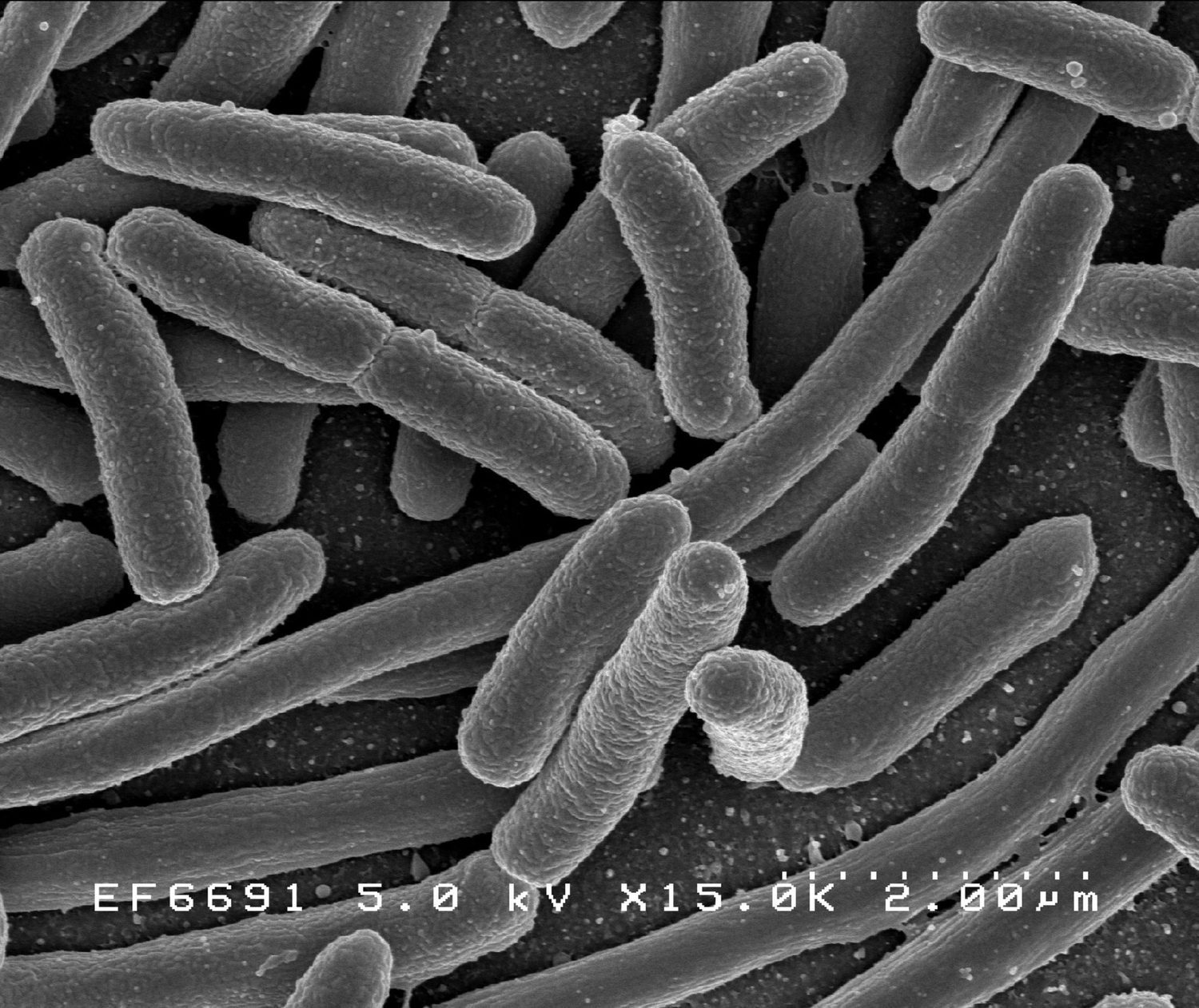
    חיידקים תחת מיקרוסקופ: דגמים אקספוננציאליים מתארים אוכלוסיות הגדלות בפקטור קבוע בכל שלב זמן
    בקטריות תחת מיקרוסקופ: מודלים אקספוננציאליים מתארים אוכלוסיות שגודלות בגורם קבוע בכל צעד זמן
    Explore · ⁨חקור⁩

    Explore an exponential curve · ⁨חקור עקום אקספוננציאלי⁩

    y = a·e^(bx) + c

    An exponential function changes by a constant factor over equal steps, so it rises (or decays) ever faster. The constant $c$ sets the horizontal asymptote it hugs. · ⁨פונקציה אקספוננציאלית משתנה על ידי גורם קבוע בשלבים שווים, ולכן היא עולה (או דועכת) בקצב תמיד גדל יותר. הקבוע $c$ קובע את האסימפטורה האופקית שהיא חובה.⁩

    Vocabulary · ⁨מילון מונחים⁩ Train · ⁨אימון⁩
    English עברית
    sequence/ˈsiːkwəns/ רצף
    arithmetic sequence/əˈrɪθmətɪk ˈsiːkwəns/ סדרה אריתמטית
    common difference/ˈkɒmən ˈdɪfrəns/ הפרש שווה
    geometric sequence/ˌdʒiːəʊˈmetrɪk ˈsiːkwəns/ סדרה גיאומטרית
    common ratio/ˈkɒmən ˈreɪʃɪəʊ/ יחס דומה
    exponential function/ˌekspəˈnenʃl ˈfʌŋkʃn/ פונקציה מעריכית
    initial value/ɪˈnɪʃl ˈvæljuː/ ערך התחלתי⟦number⟧
    base/beɪs/ בסיס
    exponential growth/ˌekspəˈnenʃl ɡrəʊθ/ צמיחה מעריכית
    exponential decay/ˌekspəˈnenʃl dɪˈkeɪ/ דעיכת מעריכית
    root/ruːt/ שורש
    exponential regression/ˌekspəˈnenʃl rɪˈɡreʃn/ רגרסיה אקספוננציאלית⟦number⟧
    natural base/ˈnætʃərəl beɪs/ בסיס טבעי
    residual plot/rɪˈsɪdʒuːəl plɒt/ גרף שאריות
    residual/rɪˈsɪdʒuːəl/ שארית
    composite function/ˈkɒmpəzɪt ˈfʌŋkʃn/ פונקציה מורכבת
    identity function/aɪˈdentɪti ˈfʌŋkʃn/ פונקציית זהות
    invertible/ɪnˈvɜːtɪbl/ הפיכה
    2.4

    Exponential Function Manipulation · ⁨עיבוד פונקציות אקספוננציאליות⁩

    Syllabus · ⁨סיילבוס⁩
    English

    Learning Objective 2.4.A: Rewrite exponential expressions in equivalent forms.

    • 2.4.A.1 The product property for exponents states that $b^m b^n = b^{(m+n)}$. Graphically, this property implies that every horizontal translation of an exponential function, $f(x) = b^{(x+k)}$, is equivalent to a vertical dilation, $f(x) = b^{(x+k)} = b^x b^k = ab^x$, where $a = b^k$.
    • 2.4.A.2 The power property for exponents states that $\left(b^m\right)^n = b^{(mn)}$. Graphically, this property implies that every horizontal dilation of an exponential function, $f(x) = b^{(cx)}$, is equivalent to a change of the base of an exponential function, $f(x) = \left(b^c\right)^x$, where $b^c$ is a constant and $c \neq 0$.
    • 2.4.A.3 The negative exponent property states that $b^{-n} = \dfrac{1}{b^n}$.
    • 2.4.A.4 The value of an exponential expression involving an exponential unit fraction, such as $b^{(1/k)}$ where $k$ is a natural number, is the $k$th root of $b$, when it exists.
    עברית

    **מטרת הלמידה 2.4.A:**改写 פונקציות מעריכיות לצורות שקולות.

    • 2.4.A.1 תכונת הכפלה למעריכים קובעת כי $b^m b^n = b^{(m+n)}$. גרפית, תכונה זו מצביעה על כך שכל הזזת אופקית של פונקציה מעריכית, $f(x) = b^{(x+k)}$, שקולה להרחבה אנכית, $f(x) = b^{(x+k)} = b^x b^k = ab^x$, כאשר $a = b^k$.
    • 2.4.A.2 תכונת החזקה למעריכים קובעת כי $\left(b^m\right)^n = b^{(mn)}$. גרפית, תכונה זו מצביעה על כך שכל הרחבה אופקית של פונקציה מעריכית, $f(x) = b^{(cx)}$, שקולה לשינוי בבסיס של פונקציה מעריכית, $f(x) = \left(b^c\right)^x$, כאשר $b^c$ הוא קבוע ו$c \neq 0$.
    • 2.4.A.3 תכונת המעריך השלילי קובעת כי $b^{-n} = \dfrac{1}{b^n}$.
    • 2.4.A.4 הערך של ביטוי מעריכי המכיל שבר יחיד מעריכי, כמו $b^{(1/k)}$ כאשר $k$ הוא מספר טבעי, הוא השורש ה$k$-י של $b$, כאשר הוא קיים.

    Source: College Board AP Course and Exam Description · ⁨מקור: תיאור הקורס והמבחן של College Board AP⁩

    English

    The exponent rules reshape exponential expressions and connect to graph transformations:

    • Product: $b^m b^n = b^{m+n}$. A horizontal shift $b^{x+k}$ equals a vertical stretch $ab^x$ with $a=b^k$.
    • Power: $(b^m)^n = b^{mn}$. A horizontal stretch $b^{cx}$ equals a base change $(b^c)^x$.
    • Negative exponent: $b^{-n}=\dfrac{1}{b^n}$.
    • Unit-fraction exponent: $b^{1/k}=\sqrt[k]{b}$ (the $k$th root 方根).
    עברית

    חוקי החזקות מעצבים ביטויים אקספוננציאליים ומקשרים להמרות גרף:

    • מכפלה: $b^m b^n = b^{m+n}$. הזזה אופקית $b^{x+k}$ שווה למתיחה אנכית $ab^x$ עם $a=b^k$.
    • חזקה: $(b^m)^n = b^{mn}$. מתיחה אופקית $b^{cx}$ שווה לשינוי בסיס $(b^c)^x$.
    • מעריך שלילי: $b^{-n}=\dfrac{1}{b^n}$.
    • מעריך כשבר יחיד: $b^{1/k}=\sqrt[k]{b}$ (השורש ה$k$).
    2.5

    Exponential Function Context and Data Modeling · ⁨הקשר פונקציה מעריכה ודגום נתונים⁩

    Syllabus · ⁨סיילבוס⁩
    English

    Learning Objective 2.5.A: Construct a model for situations involving proportional output values over equal-length input-value intervals.

    • 2.5.A.1 Exponential functions model growth patterns where successive output values over equal-length input-value intervals are proportional. When the input values are whole numbers, exponential functions model situations of repeated multiplication of a constant to an initial value.
    • 2.5.A.2 A constant may need to be added to the dependent variable values of a data set to reveal a proportional growth pattern.
    • 2.5.A.3 An exponential function model can be constructed from an appropriate ratio and initial value or from two input-output pairs. The initial value and the base can be found by solving a system of equations resulting from the two input-output pairs.
    • 2.5.A.4 Exponential function models can be constructed by applying transformations to $f(x) = ab^x$ based on characteristics of a contextual scenario or data set.
    • 2.5.A.5 Exponential function models can be constructed for a data set with technology using exponential regressions.
    • 2.5.A.6 The natural base $e$, which is approximately $2.718$, is often used as the base in exponential functions that model contextual scenarios.
    עברית

    מטרת הלמידה 2.5.A: בניית מודל למצבים המכילים ערכי פלט פרופורציונליים על פני רווחי ערכי קלט בעלי אורך שווה.

    • 2.5.A.1 פונקציות מעריכיות מדגשות דפוסי גידול שבהם ערכי פלט רצופים על פני רווחי ערכי קלט בעלי אורך שווה הם פרופורציונליים. כאשר ערכי הקלט הם מספרים שלמים, פונקציות מעריכיות מדגשות מצבים של הכפלה חוזרת של קבוע לערך התחלתי.
    • 2.5.A.2 ייתכן שיש להוסיף קבוע לערכי משתנה התלוי במ数据集 כדי לחשוף דפוס גידול פרופורציונלי.
    • 2.5.A.3 ניתן לבנות מודל פונקציה מעריכית מתוך יחס מתאים וערך התחלתי, או מתוך שני זוגות קלט-פלט. את הערך ההתחלתי והבסיס ניתן למצוא על ידי פתרון מערכת משוואות הנובעת משני זוגות הקלט-פלט.
    • 2.5.A.4 ניתן לבנות מודלים לפונקציות מעריכיות על ידי יישום טרנספורמציות ל $f(x) = ab^x$ בהתבסס על מאפיינים של תרחיש רלוונטי או ערכי נתונים.
    • 2.5.A.5 ניתן לבנות מודלים לפונקציות מעריכיות עבור סט נתונים באמצעות טכנולוגיה, על בסיס רגרסיה מעריכית.
    • 2.5.A.6 הבסיס הטבעי $e$, השווה בקירוב ל $2.718$, משמש לעיתים קרובות כבסיס בפונקציות מעריכיות המדגמות תרחישים רלוונטיים.

    Source: College Board AP Course and Exam Description · ⁨מקור: תיאור הקורס והמבחן של College Board AP⁩

    English

    Exponentials model quantities that grow by a constant proportion over equal intervals (repeated multiplication).

    • Build a model from a ratio and an initial value, or from two points (solve the system for $a$ and $b$).
    • Sometimes a constant must be added to the data to reveal the proportional pattern.
    • Use exponential regression 指数回归 on technology to fit a data set.
    • The natural base 自然底数 $e\approx 2.718$ is the standard base for real-world models.
    עברית

    פונקציות מעריכות מדגמות כמויות הגודלות ביחס קבוע על פני מרווחים שווים (כפל חוזר).

    • לבנות דגם מתוך יחס וערך התחלתי, או מתוך שתי נקודות (פתרון המערכת עבור $a$ ו$b$).
    • לעיתים יש להוסיף קבוע לנתונים כדי לחשוף את הדפוס היחסי.
    • השתמש ברגרסיה מעריכה בתוכנה כדי להתאים סט נתונים.
    • הבסיס הטבעי $e\approx 2.718$ הוא הבסיס הסטנדרטי לדגמים בעולם האמיתי.
    2.6

    Competing Function Model Validation · ⁨אימות דגם פונקציות מתחרות⁩

    Syllabus · ⁨סיילבוס⁩
    English

    Learning Objective 2.6.A: Construct linear, quadratic, and exponential models based on a data set.

    • 2.6.A.1 Two variables in a data set that demonstrate a slightly changing rate of change can be modeled by linear, quadratic, and exponential function models.
    • 2.6.A.2 Models can be compared based on contextual clues and applicability to determine which model is most appropriate.

    Learning Objective 2.6.B: Validate a model constructed from a data set.

    • 2.6.B.1 A model is justified as appropriate for a data set if the graph of the residuals of a regression, the residual plot, appear without pattern.
    • 2.6.B.2 The difference between the predicted and actual values is the error in the model. Depending on the data set and context, it may be more appropriate to have an underestimate or overestimate for any given interval.
    עברית

    מטרות לימוד 2.6.A: בניית מודלים ליניאריים, ריבועיים ומעריכיים על בסיס סט נתונים.

    • 2.6.A.1 שני משתנים בסט נתונים המציגים קצב שינוי משתנה מעט יכולים להיות מדומים על ידי מודלים לפונקציות ליניאריות, ריבועיות ומעריכיות.
    • 2.6.A.2 ניתן להשוות בין מודלים בהתבסס על רמזים מהתרחיש הרלוונטי וביצועיות כדי לקבוע איזה מודל הוא המתאים ביותר.

    מטרות לימוד 2.6.B: אימות מודל שנבנה מסט נתונים.

    • 2.6.B.1 מודל נחשב מתאים לסט נתונים אם גרף שאריות הרגרסיה, כלומר גרף האשריות, מוצג ללא דפוס.
    • 2.6.B.2 ההפרש בין הערכים המנובאים לערכים האמיתיים הוא השגיאה במודל. בהתבסס על סט הנתונים והתרחיש, עשוי להיות יותר מתאים להשיג הערכת חיסרון או הערכת יתר לכל מרווח נתון.

    Source: College Board AP Course and Exam Description · ⁨מקור: תיאור הקורס והמבחן של College Board AP⁩

    English

    When a rate of change shifts only slightly, linear, quadratic, and exponential models may all seem to fit. Choose using context and fit quality:

    • A model is appropriate if its residual plot 残差图 shows no pattern (a residual 残差 is actual minus predicted).
    • The error is the gap between predicted and actual; context decides whether an over- or under-estimate is safer.
    עברית

    כאשר קצב השינוי משתנה רק במעט, דגמים ליניאריים, ריבועיים ומעריכים עשויים להיראות כולם מתאימים. בחר בהתאם להקשר ולאיכות ההתאמה:

    • הדגם מתאים אם גרף השאריות שלו מראה אין דפוס (השארית היא הערך בפועל פחות הערך המוצא).
    • השגיאה היא הפער בין המוצא לבין בפועל; ההקשר קובע האם הערכה גבוהה או נמוכה בטוחה יותר.
    2.7

    Composition of Functions · ⁨הרכבת פונקציות⁩

    Syllabus · ⁨סיילבוס⁩
    English

    Learning Objective 2.7.A: Evaluate the composition of two or more functions for given values.

    • 2.7.A.1 If $f$ and $g$ are functions, the composite function $f \circ g$ maps a set of input values to a set of output values such that the output values of $g$ are used as input values of $f$. For this reason, the domain of the composite function is restricted to those input values of $g$ for which the corresponding output value is in the domain of $f$. $(f \circ g)(x)$ can also be represented as $f(g(x))$.
    • 2.7.A.2 Values for the composite function $f \circ g$ can be calculated or estimated from the graphical, numerical, analytical, or verbal representations of $f$ and $g$ by using output values from $g$ as input values for $f$.
    • 2.7.A.3 The composition of functions is not commutative; that is, $f \circ g$ and $g \circ f$ are typically different functions; therefore, $f(g(x))$ and $g(f(x))$ are typically different values.
    • 2.7.A.4 If the function $f(x) = x$ is composed with any function $g$, the resulting composite function is the same as $g$; that is, $g(f(x)) = f(g(x)) = g(x)$. The function $f(x) = x$ is called the identity function. When composing two functions, the identify function acts in the same way as $0$, the additive identity, when adding two numbers and $1$, the multiplicative identity, when multiplying two numbers.

    Learning Objective 2.7.B: Construct a representation of the composition of two or more functions.

    • 2.7.B.1 Function composition is useful for relating two quantities that are not directly related by an existing formula.
    • 2.7.B.2 When analytic representations of the functions $f$ and $g$ are available, an analytic representation of $f(g(x))$ can be constructed by substituting $g(x)$ for every instance of $x$ in $f$.
    • 2.7.B.3 A numerical or graphical representation of $f \circ g$ can often be constructed by calculating or estimating values for $(x, f(g(x)))$.

    Learning Objective 2.7.C: Rewrite a given function as a composition of two or more functions.

    • 2.7.C.1 Functions given analytically can often be decomposed into less complicated functions. When properly decomposed, the variable in one function should replace each instance of the function with which it was composed.
    • 2.7.C.2 An additive transformation of a function, $f$, that results in vertical and horizontal translations can be understood as the composition of $g(x) = x + k$ with $f$.
    • 2.7.C.3 A multiplicative transformation of a function, $f$, that results in vertical and horizontal dilations can be understood as the composition of $g(x) = kx$ with $f$.
    עברית

    מטרות לימוד 2.7.A: חישוב הרכבה של שתי פונקציות או יותר עבור ערכים נתונים.

    • 2.7.A.1 אם $f$ ו $g$ הן פונקציות, הפונקציה המורכבת $f \circ g$ מפתחת סט של ערכי קלט לסט של ערכי פלט כך שערכי הפלט של $g$ משמשים כערכי קלט של $f$. מטעם זה, התחום של הפונקציה המורכבת מוגבל לערכי הקלט של $g$ עבורם ערך הפלט המתאים נמצא בתחום ההגדרה של $f$. $(f \circ g)(x)$ ניתן גם לייצג כ $f(g(x))$.
    • 2.7.A.2 ניתן לחשב או להעריך ערכים עבור הפונקציה המורכבת $f \circ g$ מתוך הייצוג הגרפי, הדידקטי, האנליטי או הלקוני של $f$ ו $g$, על ידי שימוש בערכי הפלט של $g$ כערכי קלט עבור $f$.
    • 2.7.A.3 הרכבת פונקציות אינה קומוטטיבית; כלומר, $f \circ g$ ו $g \circ f$ הן בדרך כלל פונקציות שונות; ולכן, $f(g(x))$ ו $g(f(x))$ הן בדרך כלל ערכים שונים.
    • 2.7.A.4 אם הפונקציה $f(x) = x$ מורכבת עם כל פונקציה אחרת $g$, הפונקציה המורכבת התוצרת היא זהה ל $g$; כלומר, $g(f(x)) = f(g(x)) = g(x)$. הפונקציה $f(x) = x$ נקראת פונקציה זהות. כאשר מרכיבים שתי פונקציות, הפונקציה הזהות פועלת באותו אופן כמו $0$, המזהה החיובי, בהוספת שני מספרים, ו $1$, המזהה הכפילתי, בהכפלת שני מספרים.

    מטרות לימוד 2.7.B: בניית ייצוג של הרכבה של שתי פונקציות או יותר.

    • 2.7.B.1 הרכבת פונקציות שימושית לקישור בין שני גדלים שאינם קשורים ישירות באמצעות נוסחה קיימת.
    • 2.7.B.2 כאשר ישנם ייצוגים אנליטיים של הפונקציות $f$ ו $g$, ניתן לבנות ייצוג אנליטי של $f(g(x))$ על ידי הצבת $g(x)$ בכל מקרה של $x$ ב $f$.
    • 2.7.B.3 ניתן לבנות לעיתים קרובות נציגה מספרית או גרפית של $f \circ g$ על ידי חישוב או הערכת ערכים עבור $(x, f(g(x)))$.

    מטרת למידה 2.7.C: לחדש פונקציה נתונה כהרכבה של שתי פונקציות או יותר.

    • 2.7.C.1 פונקציות הנתונות אנליטית יכולות לעיתים להיפרד לפונקציות פשוטות יותר. כאשר הפירוק בוצע בצורה הנכונה, המשתנה בפונקציה אחת צריך להחליף כל מופע של הפונקציה שבה הוא הורכב.
    • 2.7.C.2 טרנספורמציה אדיטיבית של פונקציה, $f$, המובילה לתרגול אנכי ואופקי, ניתנת להבנה כהרכבה של $g(x) = x + k$ עם $f$.
    • 2.7.C.3 טרנספורמציה מכפלתיתית של פונקציה, $f$, המובילה לקפיאה ודילטציה אנכיים ואופקיים, ניתנת להבנה כהרכבה של $g(x) = kx$ עם $f$.

    Source: College Board AP Course and Exam Description · ⁨מקור: תיאור הקורס והמבחן של College Board AP⁩

    English

    The composite function 复合函数 $(f\circ g)(x)=f(g(x))$ feeds $g$'s output into $f$. Its domain is the inputs of $g$ whose outputs lie in $f$'s domain.

    • Composition is not commutative: $f(g(x))$ and $g(f(x))$ usually differ.
    • To build $f(g(x))$ analytically, substitute $g(x)$ for every $x$ in $f$.
    • The identity function 恒等函数 $f(x)=x$ leaves any function unchanged under composition.
    • A function can also be decomposed into simpler pieces – useful for seeing an additive shift as composing with $x+k$, or a dilation as composing with $kx$.
    עברית

    הפונקציה המורכבת $(f\circ g)(x)=f(g(x))$ מזינה את תוצאת $g$ לתוך $f$. תחום ההגדרה שלה הוא הקלט של $g$ שתוצאותיו נמצאות בתחום ההגדרה של $f$.

    פונקציה כמכונה; ההופך שלה מפעילה את המכונה לאחור
    פונקציה כמכונה; ההופך שלה מפעילה את המכונה לאחור
    • הרכבה אינה קומוטטיבית: $f(g(x))$ ו$g(f(x))$ בדרך כלל שונים.
    • כדי לבנות את $f(g(x))$ אנליטית, החלף את $g(x)$ בכל $x$ בתוך $f$.
    • פונקציית הזהות $f(x)=x$ משאירה כל פונקציה ללא שינוי תחת הרכבה.
    • פונקציה יכולה להיות גם מופרדת לחלקים פשוטים יותר – דבר שימושי להבנת הזזה כאלכסונית כהרכבה עם $x+k$, או התרחבות כהרכבה עם $kx$.
    בובות מטריושקה: הרכבת פונקציות משתלבת שכבות — מחשבים קודם את הפנימי
    בובות מטריושקה: הרכבת פונקציות משתלבת שכבות — מחשבים קודם את הפנימי
    2.8

    Inverse Functions · ⁨פונקציות הפוכות⁩

    Syllabus · ⁨סיילבוס⁩
    English

    Learning Objective 2.8.A: Determine the input-output pairs of the inverse of a function.

    • 2.8.A.1 On a specified domain, a function, $f$, has an inverse function, or is invertible, if each output value of $f$ is mapped from a unique input value. The domain of a function may be restricted in many ways to make the function invertible.
    • 2.8.A.2 An inverse function can be thought of as a reverse mapping of the function. An inverse function, $f^{-1}$, maps the output values of a function, $f$, on its invertible domain to their corresponding input values; that is, if $f(a) = b$, then $f^{-1}(b) = a$. Alternately, on its invertible domain, if a function consists of input-output pairs $(a, b)$, then the inverse function consists of input-output pairs $(b, a)$.

    Learning Objective 2.8.B: Determine the inverse of a function on an invertible domain.

    • 2.8.B.1 The composition of a function, $f$, and its inverse function, $f^{-1}$, is the identity function; that is, $f\left(f^{-1}(x)\right) = f^{-1}(f(x)) = x$.
    • 2.8.B.2 On a function's invertible domain, the function's range and domain are the inverse function's domain and range, respectively. The inverse of the table of values of $y = f(x)$ can be found by reversing the input-output pairs; that is, $(a, b)$ corresponds to $(b, a)$.
    • 2.8.B.3 The inverse of the graph of the function $y = f(x)$ can be found by reversing the roles of the $x$- and $y$-axes; that is, by reflecting the graph of the function over the graph of the identity function $h(x) = x$.
    • 2.8.B.4 The inverse of the function can be found by determining the inverse operations to reverse the mapping. One method for finding the inverse of the function $f$ is reversing the roles of $x$ and $y$ in the equation $y = f(x)$, then solving for $y = f^{-1}(x)$.
    • 2.8.B.5 In addition to limiting the domain of a function to obtain an inverse function, contextual restrictions may also limit the applicability of an inverse function.
    עברית

    מטרת למידה 2.8.A: לקבוע זוגות קלט-פלט ההפוך של פונקציה.

    • 2.8.A.1 בתחום מוגדר ספציפי, לפונקציה, $f$, יש פונקציה הפוכה, או שהיא הופכת, אם כל ערך פלט של $f$ מקודד מערך קלט ייחודי. ניתן להגביר את תחום הפונקציה בדרכים רבות כדי להפוך אותה להפכה.
    • 2.8.A.2 פונקציה הפוכה ניתן לחשוב עליה כהפך הקידוד של הפונקציה. פונקציה הפוכה, $f^{-1}$, מקידדת את ערכי הפלט של פונקציה, $f$, בתחומה ההפוך, לערכי הקלט המתאימים שלהן; כלומר, אם $f(a) = b$, אז $f^{-1}(b) = a$. חלופתית, בתחומה ההפוך, אם פונקציה מורכבת מזוגות קלט-פלט $(a, b)$, אזי הפונקציה ההפוכה מורכבת מזוגות קלט-פלט $(b, a)$.

    מטרת למידה 2.8.B: לקבוע את ההפוך של פונקציה בתחום הפוך.

    • 2.8.B.1 ההרכבה של פונקציה, $f$, והפונקציה ההפוכה שלה, $f^{-1}$, היא הפונקציה הזהות; כלומר, $f\left(f^{-1}(x)\right) = f^{-1}(f(x)) = x$.
    • 2.8.B.2 בתחום ההפוך של פונקציה, התחום והטווח שלה הם, בהתאמה, הטווח והתחום של הפונקציה ההפוכה. ניתן למצוא את ההפוך של טבלת הערכים של $y = f(x)$ על ידי הפיכת זוגות הקלט-פלט; כלומר, $(a, b)$ מתאים ל$(b, a)$.
    • 2.8.B.3 ניתן למצוא את ההפוך של הגרף של הפונקציה $y = f(x)$ על ידי הפיכת התפקידים של ציר ה-$x$ וציר ה-$y$; כלומר, על ידי השתקפות הגרף של הפונקציה לאורך גרף הפונקציה זהות $h(x) = x$.
    • 2.8.B.4 ניתן למצוא את ההפוך של הפונקציה על ידי קביעת הפעולות ההפוכות להפוך את הקידוד. שיטה אחת למצוא את ההפוך של הפונקציה $f$ היא להפוך את התפקידים של $x$ ו$y$ במשוואה $y = f(x)$, ולאחר מכן לפתור עבור $y = f^{-1}(x)$.
    • 2.8.B.5 בנוסף להגבלת תחום הפונקציה כדי לקבל פונקציה הפוכה, הגבלות הקשרי גם הן עשויות להגביל את הרלוונטיות של פונקציה הפוכה.

    Source: College Board AP Course and Exam Description · ⁨מקור: תיאור הקורס והמבחן של College Board AP⁩

    English
    Inverse functions are a reflection
    Exponential & logarithm are inverses

    A function is invertible 可逆 on a domain where each output comes from a unique input (you may restrict the domain to force this). The inverse function 反函数 $f^{-1}$ reverses the mapping: if $f(a)=b$ then $f^{-1}(b)=a$.

    • $f\big(f^{-1}(x)\big)=f^{-1}\big(f(x)\big)=x$ (composition gives the identity).
    • Domain and range swap: reverse each $(a,b)$ to $(b,a)$ in a table; reflect the graph over the line $y=x$.
    • To find a formula: swap $x$ and $y$ in $y=f(x)$, then solve for $y$. Context may further limit where the inverse applies.
    עברית
    פונקציות הפוכות הן סימטריה
    פונקציות מעריכיות ולוגריתמיות הן הפוכות

    פונקציה היא הפיכה בתחום שבו כל ערך יוצא נובע מתוך קלט ייחודי (ניתן לצמצם את התחום כדי להכריח זאת). ה-פונקציה ההפוכה $f^{-1}$ מהפכת את היחס: אם $f(a)=b$ אזי $f^{-1}(b)=a$.

    • $f\big(f^{-1}(x)\big)=f^{-1}\big(f(x)\big)=x$ (ההרכבה נותנת זהות).
    • תחום הגדרה וטווח מתחלפים: הפכו כל ⟨$(a,b)$⟩ ל$(b,a)$ בטבלה; השתקפו את הגרף על פני הקו $y=x$.
    • למצוא נוסחה: החלף בין $x$ ל-$y$ ב-$y=f(x)$, ולאחר מכן פתור עבור $y$. ההקשר עשוי להגביל נוספים את האזור שבו ההיפוך תקף.
    Vocabulary · ⁨מילון מונחים⁩ Train · ⁨אימון⁩
    English עברית
    inverse function/ɪnˈvɜːs ˈfʌŋkʃn/ פונקציה הפוכה
    logarithm/ˈlɒɡərɪθəm/ לוגריתם
    common logarithm/ˈkɒmən ˈlɒɡərɪθəm/ לוגריתם עשרוני
    natural logarithm/ˈnætʃərəl ˈlɒɡərɪθəm/ לוגריתם טבעי
    logarithmic function/ˌlɒɡəˈrɪθmɪk ˈfʌŋkʃn/ פונקציית לוגריתם⟦number⟧
    change-of-base/tʃeɪndʒ ɒv beɪs/ שינוי בסיס⟦number⟧
    semi-log plot/ˈsemi lɒɡ plɒt/ גרף סמי-לוגaritmic⟦number⟧
    2.9

    Logarithmic Expressions · ⁨ביטויים לוגاريتمي⁩

    Syllabus · ⁨סיילבוס⁩
    English

    Learning Objective 2.9.A: Evaluate logarithmic expressions.

    • 2.9.A.1 The logarithmic expression $\log_b c$ is equal to, or represents, the value that the base $b$ must be exponentially raised to in order to obtain the value $c$. That is, $\log_b c = a$ if and only if $b^a = c$, where $a$ and $c$ are constants, $b > 0$, and $b \neq 1$. (when the base of a logarithmic expression is not specified, it is understood as the common logarithm with a base of $10$)
    • 2.9.A.2 The values of some logarithmic expressions are readily accessible through basic arithmetic while other values can be estimated through the use of technology.
    • 2.9.A.3 On a logarithmic scale, each unit represents a multiplicative change of the base of the logarithm. For example, on a standard scale, the units might be $0, \; 1, \; 2, \; \ldots$, while on a logarithmic scale, using logarithm base $10$, the units might be $10^0, \; 10^1, \; 10^2, \; \ldots$.
    עברית

    מטרת למידה 2.9.A: לחשב ביטויים לוגריתמיים.

    • 2.9.A.1 הביטוי הלוגריתמי $\log_b c$ שווה, או מייצג, את הערך שבו הבסיס $b$ חייב להיות מוגבה בחזקה אקספוננציאלית כדי לקבל את הערך $c$. כלומר, $\log_b c = a$ אם ורק אם $b^a = c$, כאשר $a$ ו$c$ הם קבועים, $b > 0$, ו$b \neq 1$. (כאשר הבסיס של ביטוי לוגריתמי אינו מצוין, הוא נחשב כלוגריתם רגיל עם בסיס של $10$)
    • 2.9.A.2 ערכים של כמה ביטויים לוגריתמיים נגישים בקלות באמצעות אריתמטיקה בסיסית, בעוד שערכים אחרים יכולים להתערכה באמצעות שימוש בטכנולוגיה.
    • 2.9.A.3 בקנה מידה לוגריתמי, כל יחידה מייצגת שינוי מכפלתיתית של בסיס הלוגריתם. לדוגמה, בקנה מידה סטנדרטי, היחידות עשויות להיות $0, \; 1, \; 2, \; \ldots$, בעוד שבקנה מידה לוגריתמי, בשימוש בבסיס לוגריתם $10$, היחידות עשויות להיות $10^0, \; 10^1, \; 10^2, \; \ldots$.

    Source: College Board AP Course and Exam Description · ⁨מקור: תיאור הקורס והמבחן של College Board AP⁩

    English

    The logarithm 对数 answers "what exponent?": $\log_b c = a$ means exactly $b^a = c$ (with $b>0,\ b\neq 1$). An unwritten base means the common logarithm 常用对数 (base $10$). On a logarithmic scale, each unit is a multiplicative step of the base (…, $10^0,10^1,10^2,$ …).

    עברית

    ה-לוגריתם מענה לשאלה "איזה חזקה?": $\log_b c = a$ פירושו בדיוק $b^a = c$ (עם $b>0,\ b\neq 1$). בסיס שלא נכתב מייצג את הלוגריתם העשרוני (בסיס $10$). בקנה מידה לוגריتمي, כל יחידה היא צעד כפוליים של הבסיס (…, $10^0,10^1,10^2,$ …).

    2.10

    Inverses of Exponential Functions · ⁨הפוכות של פונקציות מעריכיות⁩

    Syllabus · ⁨סיילבוס⁩
    English

    Learning Objective 2.10.A: Construct representations of the inverse of an exponential function with an initial value of 1.

    • 2.10.A.1 The general form of a logarithmic function is $f(x) = a\log_b x$, with base $b$, where $b > 0$, $b \neq 1$, and $a \neq 0$.
    • 2.10.A.2 The way in which input and output values vary together have an inverse relationship in exponential and logarithmic functions. Output values of general-form exponential functions change proportionately as input values increase in equal-length intervals. However, input values of general-form logarithmic functions change proportionately as output values increase in equal-length intervals. Alternately, exponential growth is characterized by output values changing multiplicatively as input values change additively, whereas logarithmic growth is characterized by output values changing additively as input values change multiplicatively.
    • 2.10.A.3 $f(x) = \log_b x$ and $g(x) = b^x$, where $b > 0$ and $b \neq 1$, are inverse functions. That is, $g(f(x)) = f(g(x)) = x$.
    • 2.10.A.4 The graph of the logarithmic function $f(x) = \log_b x$, where $b > 0$ and $b \neq 1$, is a reflection of the graph of the exponential function $g(x) = b^x$, where $b > 0$ and $b \neq 1$, over the graph of the identity function $h(x) = x$.
    • 2.10.A.5 If $(s, \; t)$ is an ordered pair of the exponential function $g(x) = b^x$, where $b > 0$ and $b \neq 1$, then $(t, \; s)$ is an ordered pair of the logarithmic function $f(x) = \log_b x$, where $b > 0$ and $b \neq 1$.
    עברית

    מטרות למידה 2.10.A: בניית תمثילים של ההפוך של פונקציה אקספוננציאלית עם ערך התחלתי של 1.

    • 2.10.A.1 הצורה הכללית של פונקציה לוגריתמית היא $f(x) = a\log_b x$, עם בסיס $b$, כאשר $b > 0$, $b \neq 1$ ו$a \neq 0$.
    • 2.10.A.2 האופן שבו ערכי קלט וערכי פלט משתנים יחדיו הוא יחס הפוך בפונקציות אקספוננציאליות ולוגריתמיות. ערכי הפלט של פונקציות אקספוננציאליות בצורה כללית משתנים פרופורציונלית כאשר ערכי הקלט גדלים בטווחים בעלי אורך שווה. עם זאת, ערכי הקלט של פונקציות לוגריתמיות בצורה כללית משתנים פרופורציונלית כאשר ערכי הפלט גדלים בטווחים בעלי אורך שווה. לחלופין, צמיחה אקספוננציאלית מאופיינת בערכי פלט המשנים את עצמם כפילתית כאשר ערכי הקלט משנים את עצמם באופן אדיטיבי, בעוד שצמיחה לוגריתמית מאופיינת בערכי פלט המשנים את עצמם אדיטיבית כאשר ערכי הקלט משנים את עצמם כפילתית.
    • 2.10.A.3 $f(x) = \log_b x$ ו$g(x) = b^x$, כאשר $b > 0$ ו$b \neq 1$, הן פונקציות הפוכות זו לזו. כלומר, $g(f(x)) = f(g(x)) = x$.
    • 2.10.A.4 הגרף של הפונקציה הלוגריתמית $f(x) = \log_b x$, כאשר $b > 0$ ו-$b \neq 1$, הוא השתקפות הגרף של הפונקציה האקספוננציאלית $g(x) = b^x$, כאשר $b > 0$ ו-$b \neq 1$, ביחס לגרף פונקציית הזהות $h(x) = x$.
    • 2.10.A.5 אם $(s, \; t)$ הוא זוג מסודר של הפונקציה האקספוננציאלית $g(x) = b^x$, כאשר $b > 0$ ו-$b \neq 1$, אזי $(t, \; s)$ הוא זוג מסודר של הפונקציה הלוגריתמית $f(x) = \log_b x$, כאשר $b > 0$ ו-$b \neq 1$.

    Source: College Board AP Course and Exam Description · ⁨מקור: תיאור הקורס והמבחן של College Board AP⁩

    English

    The logarithm is the inverse of the exponential: $y=b^x$ and $y=\log_b x$ undo each other, so their graphs are reflections over $y=x$. Hence $\log_b(b^x)=x$ and $b^{\log_b x}=x$. The natural logarithm 自然对数 $\ln x = \log_e x$ is the inverse of $e^x$.

    עברית

    הלוגריתם הוא ההפוכה של הפונקציה המעריכית: $y=b^x$ ו-$y=\log_b x$ מבטלים זה את זה, ולכן גרפיהם הם סימטריה ביחס ל-$y=x$. מכאן ש-$\log_b(b^x)=x$ ו-$b^{\log_b x}=x$. ה-לוגריתם הטבעי $\ln x = \log_e x$ הוא ההפוכה של $e^x$.

    e^x ו-ln x הם סימטריה זה של זה בקו y = x
    e^x ו-ln x הם סימטריה זה של בקו y = x
    2.11

    Logarithmic Functions · ⁨פונקציות לוגריתמיות⁩

    Syllabus · ⁨סיילבוס⁩
    English

    Learning Objective 2.11.A: Identify key characteristics of logarithmic functions.

    • 2.11.A.1 The domain of a logarithmic function in general form is any real number greater than zero, and its range is all real numbers.
    • 2.11.A.2 Because logarithmic functions are inverses of exponential functions, logarithmic functions are also always increasing or always decreasing, and their graphs are either always concave up or always concave down. Consequently, logarithmic functions do not have extrema except on a closed interval, and their graphs do not have points of inflection.
    • 2.11.A.3 The additive transformation function $g(x) = f(x + k)$, where $k \neq 0$, of a logarithmic function $f$ in general form does not have input values that are proportional over equal-length output-value intervals. However, if the input values of the additive transformation function, $g(x) = f(x + k)$, of any function $f$ are proportional over equal-length output value intervals, then $f$ is logarithmic.
    • 2.11.A.4 With their limited domain, logarithmic functions in general form are vertically asymptotic to $x = 0$, with an end behavior that is unbounded. That is, for a logarithmic function in general form, $\lim\limits_{x \to 0^+} a\log_b x = \pm\infty$ and $\lim\limits_{x \to \infty} a\log_b x = \pm\infty$.
    עברית

    מטרות לימוד 2.11.A: זיהוי מאפיינים מרכזיים של פונקציות לוגריתמיות.

    • 2.11.A.1 תחום ההגדרה של פונקציה לוגריתמית בצורה כללית הוא כל המספרים הממשיים הגדולים מאפס, והטווח שלה הוא כל המספרים הממשיים.
    • 2.11.A.2 מכיוון שפונקציות לוגריתמיות הן ההופכות של פונקציות אקספוננציאליות, פונקציות לוגריתמיות הן גם תמיד עולות או תמיד יורדות, וגרפים שלהן הם או תמיד קעורים כלפי מעלה או תמיד קעורים כלפי מטה. כתוצאה מכך, לפונקציות לוגריתמיות אין נקודות קיצון אלא בתחום סגור, וגרפים שלהן אינם כוללים נקודות חילוף.
    • 2.11.A.3 פונקציית ההמרה האדיטיבית $g(x) = f(x + k)$, כאשר $k \neq 0$, של פונקציה לוגריתמית $f$ בצורה כללית אינה בעלת ערכי קלט פרופורציונליים על פני רווחי ערך יציאת באורך שווה. עם זאת, אם ערכי הקלט של פונקציית ההמרה האדיטיבית, $g(x) = f(x + k)$, של כל פונקציה $f$ הם פרופורציונליים על פני רווחי ערך יציאה באורך שווה, אזי $f$ היא לוגריתמית.
    • 2.11.A.4 עם תחום הגדרה מוגבל, פונקציות לוגריתמיות בצורה כללית הן אספטוטיות אנכית ל-$x = 0$, עם התנהגות בסיום שאינה מוגבלת. כלומר, עבור פונקציית לוגריתם בצורה כללית, $\lim\limits_{x \to 0^+} a\log_b x = \pm\infty$ ו-$\lim\limits_{x \to \infty} a\log_b x = \pm\infty$.

    Source: College Board AP Course and Exam Description · ⁨מקור: תיאור הקורס והמבחן של College Board AP⁩

    English

    The logarithmic function 对数函数 $f(x)=\log_b x$ has domain $x>0$ and range all reals. It is always increasing (for $b>1$) or always decreasing (for $0), always concave one way, with a vertical asymptote at $x=0$ – the mirror image of the exponential's horizontal asymptote. It grows very slowly for large $x$.

    עברית

    הפונקציה הלוגריתמית $f(x)=\log_b x$ היא בעלת תחום $x>0$ וטווח של כל המספרים הממשיים. היא תמיד עולה (עבור $b>1$) או תמיד יורדת (עבור $0), תמיד קעורה לכיוון אחד, עם אסימפטוטה אנכית ב-$x=0$ – שהיא הדמות המשתקפת של האסימפטוטה האופקית של הפונקציה האקספוננציאלית. היא צומחת מאוד לאט עבור ערכים גדולים של $x$.

    Explore · ⁨חקור⁩

    Explore a logarithmic curve · ⁨חקור עקום לוגריתמי⁩

    y = a·ln(x − b) + c

    A logarithm is the inverse of an exponential: it grows without bound but ever slower, with a vertical asymptote where its input hits zero. · ⁨לוגריתם הוא ההופך של אקספוננציאל: הוא צומח ללא גבול אך בקצב תמיד איטי יותר, עם אסימפטורה אנכית כאשר הקלט שלו מגיע לאפס.⁩

    2.12

    Logarithmic Function Manipulation · ⁨עיבוד פונקציות לוגריתמיות⁩

    Syllabus · ⁨סיילבוס⁩
    English

    Learning Objective 2.12.A: Rewrite logarithmic expressions in equivalent forms.

    • 2.12.A.1 The product property for logarithms states that $\log_b(xy) = \log_b x + \log_b y$. Graphically, this property implies that every horizontal dilation of a logarithmic function, $f(x) = \log_b(kx)$, is equivalent to a vertical translation, $f(x) = \log_b(kx) = \log_b k + \log_b x = a + \log_b x$, where $a = \log_b k$.
    • 2.12.A.2 The power property for logarithms states that $\log_b x^n = n\log_b x$. Graphically, this property implies that raising the input of a logarithmic function to a power, $f(x) = \log_b x^k$, results in a vertical dilation, $f(x) = \log_b x^k = k\log_b x$.
    • 2.12.A.3 The change of base property for logarithms states that $\log_b x = \dfrac{\log_a x}{\log_a b}$, where $a > 0$ and $a \neq 1$. This implies that all logarithmic functions are vertical dilations of each other.
    • 2.12.A.4 The function $f(x) = \ln x$ is a logarithmic function with the natural base $e$; that is, $\ln x = \log_e x$.
    עברית

    מטרות לימוד 2.12.A: כתיבת ביטויים לוגריתמיים בצורות שקולות.

    • 2.12.A.1 משפט המכפלה ללוגריתמים קובע כי $\log_b(xy) = \log_b x + \log_b y$. גרפית, משפט זה מצביע על כך שכל הרחבה אופקית של פונקציה לוגריתמית, $f(x) = \log_b(kx)$, שקולה להזזה אנכית, $f(x) = \log_b(kx) = \log_b k + \log_b x = a + \log_b x$, כאשר $a = \log_b k$.
    • 2.12.A.2 משפט החזקה ללוגריתמים קובע כי $\log_b x^n = n\log_b x$. גרפית, משפט זה מצביע על כך שהרמת הקלט של פונקציה לוגריתמית לחזקה, $f(x) = \log_b x^k$, מובילה להרחבה אנכית, $f(x) = \log_b x^k = k\log_b x$.
    • 2.12.A.3 משפט שינוי הבסיס ללוגריתמים קובע כי $\log_b x = \dfrac{\log_a x}{\log_a b}$, כאשר $a > 0$ ו-$a \neq 1$. משפט זה מצביע על כך שכל הפונקציות הלוגריתמיות הן הרחבות אנכיות זו של זו.
    • 2.12.A.4 הפונקציה $f(x) = \ln x$ היא פונקציה לוגריתמית עם בסיס טבעי $e$; כלומר, $\ln x = \log_e x$.

    Source: College Board AP Course and Exam Description · ⁨מקור: תיאור הקורס והמבחן של College Board AP⁩

    English

    The log properties reverse the exponent rules:

    $$\log_b(xy)=\log_b x+\log_b y,\quad \log_b\!\frac{x}{y}=\log_b x-\log_b y,\quad \log_b(x^n)=n\log_b x.$$
    The change-of-base 换底 formula lets you compute any log with technology: $\log_b x = \dfrac{\log x}{\log b}=\dfrac{\ln x}{\ln b}$.

    עברית

    תכונות הלוגריתם הופכות את חוקי החזקות:

    $$\log_b(xy)=\log_b x+\log_b y,\quad \log_b\!\frac{x}{y}=\log_b x-\log_b y,\quad \log_b(x^n)=n\log_b x.$$
    נוסחת החלפת בסיס מאפשרת לחשב לוגריתם כלשהו באמצעות מכשיר: $\log_b x = \dfrac{\log x}{\log b}=\dfrac{\ln x}{\ln b}$.

    2.13

    Exponential and Logarithmic Equations and Inequalities · ⁨משוואות ואי-שוויון אקספוננציאליים ולוגריתמיים⁩

    Syllabus · ⁨סיילבוס⁩
    English

    Learning Objective 2.13.A: Solve exponential and logarithmic equations and inequalities.

    • 2.13.A.1 Properties of exponents, properties of logarithms, and the inverse relationship between exponential and logarithmic functions can be used to solve equations and inequalities involving exponents and logarithms.
    • 2.13.A.2 When solving exponential and logarithmic equations found through analytical or graphical methods, the results should be examined for extraneous solutions precluded by the mathematical or contextual limitations.
    • 2.13.A.3 Logarithms can be used to rewrite expressions involving exponential functions in different ways that may reveal helpful information. Specifically, $b^x = c^{(\log_c b)(x)}$.

    Learning Objective 2.13.B: Construct the inverse function for exponential and logarithmic functions.

    • 2.13.B.1 The function $f(x) = ab^{(x-h)} + k$ is a combination of additive transformations of an exponential function in general form. The inverse of $y = f(x)$ can be found by determining the inverse operations to reverse the mapping.
    • 2.13.B.2 The function $f(x) = a\log_b(x - h) + k$ is a combination of additive transformations of a logarithmic function in general form. The inverse of $y = f(x)$ can be found by determining the inverse operations to reverse the mapping.
    עברית

    מטרות לימוד 2.13.A: פתרון משוואות ואי-שוויונות אקספוננציאליים ולוגריתמיים.

    • 2.13.A.1 ניתן להשתמש במאפייני חזקות, מאפייני לוגריתמים ובקשר ההופכי בין פונקציות אקספוננציאליות ולוגריתמיות כדי לפתור משוואות ואי-שוויונים המכילים חזקות ולוגריתמים.
    • 2.13.A.2 בפתרון משוואות אקספוננציאליות ולוגריתמיות שמצאו דרך שיטות אנליטיות או גרפיות, יש לבדוק את התוצאות בנוגע לפתרונים חיצוניים שנשללו בגלל מגבלות מתמטיות או קונטקסטואליות.
    • 2.13.A.3 לוגריתמים יכולים לשמש כדי לקבוע מחדש ביטויים המכילים פונקציות אקספוננציאליות בדרכים שונות שעשו לחשוף מידע מועיל. ספציפית, $b^x = c^{(\log_c b)(x)}$.

    מטרות לימוד 2.13.B: בניית פונקציית ההופך לפונקציות אקספוננציאליות ולוגריתמיות.

    • 2.13.B.1 הפונקציה $f(x) = ab^{(x-h)} + k$ היא שילוב של תמורות חיבוריות לפונקצייה אקספוננציאלית בצורה כללית. ההופך של $y = f(x)$ ניתן למצוא על ידי קביעת הפעולות ההופכות כדי להפיך את ההתאמה.
    • 2.13.B.2 הפונקציה $f(x) = a\log_b(x - h) + k$ היא שילוב של תמורות חיבוריות לפונקצייה לוגריתמית בצורה כללית. ההופך של $y = f(x)$ ניתן למצוא על ידי קביעת הפעולות ההופכות כדי להפיך את ההתאמה.

    Source: College Board AP Course and Exam Description · ⁨מקור: תיאור הקורס והמבחן של College Board AP⁩

    English

    To solve, use the fact that exponentials and logs are inverses:

    • Isolate the exponential, then take a log of both sides (bring the exponent down with the power property).
    • Isolate the log, then exponentiate both sides.
    • Always check for extraneous solutions – the argument of a log must stay positive.

    Worked example. Solve $2\cdot3^x=54$. Divide by $2$: $3^x=27=3^3$, so $x=3$. When the sides are not tidy powers, take logs instead: $5^x=20$ gives $x=\dfrac{\ln 20}{\ln 5}\approx1.86$.

    עברית

    כדי לפתור, השתמש בעובדה שאקספוננטים ולוגריתמים הם פונקציות הפוכות:

    • הפרד את האקספוננט, ולאחר מכן נגז לוגריתם לשני הצדדים (הורד את המעריך באמצעות תכונת החזקה).
    • הפרד את הלוגריתם, ולאחר מכן הרם את שני הצדדים כמעריכים.
    • תמיד בדוק קיום של פתרונות זרים – הטיעון של לוגריתם חייב להישאר חיובי.

    דוגמה מוצעת. פתור $2\cdot3^x=54$. חלק ב-$2$: $3^x=27=3^3$, ולכן $x=3$. כאשר הצדדים אינם מעריכים מסודרים, נגז לוגריתם במקום זאת: $5^x=20$ מוביל ל-$x=\dfrac{\ln 20}{\ln 5}\approx1.86$.

    2.14

    Logarithmic Function Context and Data Modeling · ⁨הקשר פונקציה לוגריתמית ודגום נתונים⁩

    Syllabus · ⁨סיילבוס⁩
    English

    Learning Objective 2.14.A: Construct a logarithmic function model.

    • 2.14.A.1 Logarithmic functions are inverses of exponential functions and can be used to model situations involving proportional growth, or repeated multiplication, where the input values change proportionally over equal-length output-value intervals. Alternately, if the output value is a whole number, it indicates how many times the initial value has been multiplied by the proportion.
    • 2.14.A.2 A logarithmic function model can be constructed from an appropriate proportion and a real zero or from two input-output pairs.
    • 2.14.A.3 Logarithmic function models can be constructed by applying transformations to $f(x) = a\log_b x$ based on characteristics of a context or data set.
    • 2.14.A.4 Logarithmic function models can be constructed for a data set with technology using logarithmic regressions.
    • 2.14.A.5 The natural logarithm function is often useful in modeling real-world phenomena.
    • 2.14.A.6 Logarithmic function models can be used to predict values for the dependent variable.
    עברית

    מטרות לימוד 2.14.A: בניית דגם פונקציה לוגריתמית.

    • 2.14.A.1 פונקציות לוגריתמיות הן הופכים של פונקציות אקספוננציאליות ויכולות לשמש לדגום מצבים המעורבים בצמיחה פרופורציונלית, או כפל חוזר, כאשר ערכי הכניסה משתנים פרופורציונלית בתוך מרווחים בעלי אורך שווה של ערכי התוצאה. לחלופין, אם ערך התוצאה הוא מספר שלם, הוא מעיד על כמה פעמים הערך ההתחלתי הוכפל בפרופורציה.
    • 2.14.A.2 דגם פונקציה לוגריתמית ניתן לבנות מהפרופורציה המתאימה ואפס אמיתי, או מזוג זוגות כניסה-תוצאה.
    • 2.14.A.3 דגמי פונקציות לוגריתמיות יכולים לבנות על ידי יישום תמורות ל-$f(x) = a\log_b x$ בהתבסס על מאפיינים של הקשר או סט נתונים.
    • 2.14.A.4 דגמי פונקציות לוגריתמיות יכולים לבנות עבור סט נתונים באמצעות טכנולוגיה, בעזרת רגרסיה לוגריתמית.
    • 2.14.A.5 פונקציית הלוגריתם הטבעי לעיתים קרובות שימושית בדגום תופעות בעולם האמיתי.
    • 2.14.A.6 דגמי פונקציות לוגריתמיים יכולים לשמש לחיזוי ערכים למשתנה התלוי.

    Source: College Board AP Course and Exam Description · ⁨מקור: תיאור הקורס והמבחן של College Board AP⁩

    English

    Logarithms model quantities that change over huge multiplicative ranges (sound, acid strength, earthquakes). Build a log model from data, and use logarithmic regression for a data set. Because a log compresses large values, it turns proportional growth into a straight-line pattern – the idea behind semi-log plots.

    עברית

    לוגריתמים מדגמים כמויותשתנות בטווחים רב-פעמיים גדולים (קול, עוצמת חומצה, רעידות אדמה). בנה דגם לוגריתמי מהנתונים, והשתמש ב-רגרסיה לוגריתמית לערכות נתונים. מכיוון שלוגריתם דוחס ערכים גדולים, הוא הופך צמיחה פרופורציונלית לדפוס קו ישר – העיקרון העומד מאחורי גרפים סמי-לוגריתמיים.

    2.15

    Semi-log Plots · ⁨גרפים סמי-לוגריתמיים⁩

    Syllabus · ⁨סיילבוס⁩
    English

    Learning Objective 2.15.A: Determine if an exponential model is appropriate by examining a semi-log plot of a data set.

    • 2.15.A.1 In a semi-log plot, one of the axes is logarithmically scaled. When the $y$-axis of a semi-log plot is logarithmically scaled, data or functions that demonstrate exponential characteristics will appear linear.
    • 2.15.A.2 An advantage of semi-log plots is that a constant never needs to be added to the dependent variable values to reveal that an exponential model is appropriate.

    Learning Objective 2.15.B: Construct the linearization of exponential data.

    • 2.15.B.1 Techniques used to model linear functions can be applied to a semi-log graph.
    • 2.15.B.2 For an exponential model of the form $y = ab^x$, the corresponding linear model for the semi-log plot is $y = (\log_n b)x + \log_n a$, where $n > 0$ and $n \neq 1$. Specifically, the linear rate of change is $\log_n b$, and the initial linear value is $\log_n a$.
    עברית

    מטרות לימוד 2.15.A: קביעה האם דגם אקספוננציאלי מתאים על ידי בדיקת גרף סמי-לוגריתמי של סט נתונים.

    • 2.15.A.1 במגרע סמי-לוגריתמי, אחד הצירים מדורג לוגריתמית. כאשר ציר ה-$y$ במגרע סמי-לוגריתמי מדורג לוגריתמית, נתונים או פונקציות המראות מאפיינים אקספוננציאליים ייראו כקוויים.
    • 2.15.A.2 יתרון הגרפים הסמי-לוגריתמיים הוא שאינו נדרש להוסיף קבוע לערכי המשתנה התלוי כדי לגלות שהדגם האקספוננציאלי מתאים.

    מטרות לימוד 2.15.B: בניית ליניארית של נתונים אקספוננציאליים.

    • 2.15.B.1 טכניקות המשמשות לדגום פונקציות ליניאריות יכולות להיות מיושמות על גרף סמי-לוגריתמי.
    • 2.15.B.2 עבור דגם אקספוננציאלי בצורת $y = ab^x$, הדגם הליניארי המתאים לגרף הסמי-לוגריתמי הוא $y = (\log_n b)x + \log_n a$, כאשר $n > 0$ ו-$n \neq 1$. במיוחד, קצב השינוי הליניארי הוא $\log_n b$, והערך ההתחלתי הליניארי הוא $\log_n a$.

    Source: College Board AP Course and Exam Description · ⁨מקור: תיאור הקורס והמבחן של College Board AP⁩

    English

    A semi-log plot 半对数图 puts the output on a logarithmic axis and the input on a normal axis. On these axes, an exponential function $y=ab^x$ becomes a straight line, because $\log y = \log a + (\log b)\,x$ is linear in $x$. So: if data look linear on a semi-log plot, an exponential model fits; the line's slope gives $\log b$ and its intercept gives $\log a$.

    עברית

    גרף סמי-לוגריתמי מציב את התוצאה על ציר לוגריתמי ואת הכניסה על ציר רגיל. על צירים אלו, פונקציה אקספוננציאלית $y=ab^x$ הופכת לקו ישר, מכיוון ש-$\log y = \log a + (\log b)\,x$ הוא ליניארי ב-$x$. לכן: אם הנתונים נראים ליניאריים בגרף סמי-לוגריתמי, דגם אקספוננציאלי מתאים; שיפוע הקו נותן $\log b$ ומחצית הישר נותנת $\log a$.

    2.15

    Exam tips · ⁨טיפים לבחינות⁩

    English
    • Distinguish arithmetic (add a common difference) from geometric (multiply a common ratio) sequences and their linear/exponential function cousins.
    • Exponential = repeated multiplication, so it eventually outgrows any linear or polynomial model.
    • The logarithm is the inverse of the exponential ($\log_b c=a\Leftrightarrow b^a=c$); use it to solve $b^x=k$.
    • Apply the log laws (product, quotient, power) and the change-of-base formula; the argument of a log must be positive.
    • On a semi-log plot an exponential model becomes a straight line.
    עברית
    • הבדל בין אריטמטי (הוספת הפרש קבוע) ל-גיאומטרי (כפל יחס קבוע) סדרות ובין הגרסאות הליניאריות/אקספוננציאליות המתאימות להן.
    • אקספוננציאל = כפל חוזר, ולכן בסוף הוא עולה על כל דגם ליניארי או פולינומי.
    • הלוגריתם הוא ההפוך של האקספוננציאל ($\log_b c=a\Leftrightarrow b^a=c$); השתמש בו כדי לפתור $b^x=k$.
    • יישם את חוקי הלוגריתם (מכפלה, מנה, חזקה) ואת נוסחת החלפת בסיס; הטיעון של לוגריתם חייב להיות חיובי.
    • בגרף סמי-לוגריתמי דגם אקספוננציאלי הופך לקו ישר.
  • 3

    Trigonometric and Polar Functions · ⁨פונקציות טריגונומטריות וקוטביות⁩

    Watch lesson · ⁨צפה בשיעור⁩
    3.1

    Periodic Phenomena · ⁨תופעות מחזוריות⁩

    Syllabus · ⁨סיילבוס⁩
    English

    Learning Objective 3.1.A: Construct graphs of periodic relationships based on verbal representations.

    • 3.1.A.1 A periodic relationship can be identified between two aspects of a context if, as the input values increase, the output values demonstrate a repeating pattern over successive equal-length intervals.
    • 3.1.A.2 The graph of a periodic relationship can be constructed from the graph of a single cycle of the relationship.

    Learning Objective 3.1.B: Describe key characteristics of a periodic function based on a verbal representation.

    • 3.1.B.1 The period of the function is the smallest positive value $k$ such that $f(x + k) = f(x)$ for all $x$ in the domain. Consequently, the behavior of a periodic function is completely determined by any interval of width $k$.
    • 3.1.B.2 The period can be estimated by investigating successive equal-length output values and finding where the pattern begins to repeat.
    • 3.1.B.3 Periodic functions take on characteristics of other functions, such as intervals of increase and decrease, different concavities, and various rates of change. However, with periodic functions, all characteristics found in one period of the function will be in every period of the function.
    עברית

    מטרת הלמידה 3.1.A: בניית גרפים של קשרים מחזוריים על בסיס ייצוגים מילוליים.

    • 3.1.A.1 ניתן לזהות קשר מחזורי בין שני היבטים של הקשר אם, כאשר ערכי הקלט עולים, ערכי הפלט מראים דפוס חוזר בתוך פרקי אורך שווה רצופים.
    • 3.1.A.2 ניתן לבנות את הגרף של קשר מחזורי מתוך הגרף של מחזור אחד בלבד של הקשר.

    מטרת הלמידה 3.1.B: תיאור מאפיינים מרכזיים של פונקציה מחזורית על בסיס ייצוג מילולי.

    • 3.1.B.1 התקופה של הפונקציה היא הערך החיובי הקטן ביותר $k$ כך ש$f(x + k) = f(x)$ לכל $x$ בתחום ההגדרה. מכאן, התנהגותה של פונקציה מחזורית נקבעת במלואה על ידי כל פרק בעל רוחב $k$.
    • 3.1.B.2 ניתן להעריך את התקופה על ידי בדיקת ערכי פלט רצופים בעלי אורך שווה וזיהוי הנקודה בה הדפוס מתחיל לחזור על עצמו.
    • 3.1.B.3 פונקציות מחזוריות לוקחות מאפיינים של פונקציות אחרות, כמו פרקי עלייה וירידה, קמבויות שונות ומשכי שינוי מגוונים. עם זאת, בפונקציות מחזוריות, כל המאפיינים שנמצאים במחזור אחד של הפונקציה יהיו קיימים בכל מחזור של הפונקציה.

    Source: College Board AP Course and Exam Description · ⁨מקור: תיאור הקורס והמבחן של College Board AP⁩

    English

    A relationship is periodic 周期性 if its output pattern repeats at regular input steps. The period 周期 is the smallest positive $k$ with $f(x+k)=f(x)$ for all $x$. You can build the whole graph by copying a single cycle 周期段, and estimate the period by finding how far apart the pattern repeats. Within each cycle a periodic function still has intervals of increase/decrease and maxima/minima.

    עברית
    התחנה החללית הבינלאומית במסלול: פונקציות טריגונומטריות וקוטביות מתארות תנועה מחזורית ועגלית
    התחנה החללית הבינלאומית במסלול: פונקציות טריגונומטריות וקוטביות מתארות תנועה מחזורית ועגלית

    יחס הוא מחזורי אם דפוס התוצאה שלו חוזר בשלבים כניסה קבועים. התקופה היא הערך החיובי הקטן ביותר $k$ כך ש-$f(x+k)=f(x)$ לכל $x$. ניתן לבנות את כל הגרף על ידי העתקת מחזור אחד, ולהעריך את התקופה על ידי מציאת המרחק בין חזרות הדפוס. בתוך כל מחזור, פונקציה מחזורית עדיין בעלת קטעים של עלייה/ירידה ומקסימומים/מינימומים.

    sin and cos wave between -1 and 1; tan breaks at 90 and 270 degrees
    גלי sin ו-cos בין -1 ל-1; tan מתפרץ ב-90 וב-270 מעלות
    גלגל הענק בווינה נגד שמיים כחולים
    כאשר גלגל הרוטב מסתובב בצורה יציבה, הגובה שלך עולה ויורם שוב ושוב — גל סינוס אמיתי לאורך זמן
    3.2

    Sine, Cosine, and Tangent · ⁨סינוס, קוסינוס וטנגנס⁩

    Syllabus · ⁨סיילבוס⁩
    English

    Learning Objective 3.2.A: Determine the sine, cosine, and tangent of an angle using the unit circle.

    • 3.2.A.1 In the coordinate plane, an angle is in standard position when the vertex coincides with the origin and one ray coincides with the positive $x$-axis. The other ray is called the terminal ray. Positive and negative angle measures indicate rotations from the positive $x$-axis in the counterclockwise and clockwise direction, respectively. Angles in standard position that share a terminal ray differ by an integer number of revolutions.
    • 3.2.A.2 The radian measure of an angle in standard position is the ratio of the length of the arc of a circle centered at the origin subtended by the angle to the radius of that same circle. For a unit circle, which has radius $1$, the radian measure is the same as the length of the subtended arc.
    • 3.2.A.3 Given an angle in standard position and a circle centered at the origin, there is a point, $P$, where the terminal ray intersects the circle. The sine of the angle is the ratio of the vertical displacement of $P$ from the $x$-axis to the distance between the origin and point $P$. Therefore, for a unit circle, the sine of the angle is the $y$-coordinate of point $P$.
    • 3.2.A.4 Given an angle in standard position and a circle centered at the origin, there is a point, $P$, where the terminal ray intersects the circle. The cosine of the angle is the ratio of the horizontal displacement of $P$ from the $y$-axis to the distance between the origin and point $P$. Therefore, for a unit circle, the cosine of the angle is the $x$-coordinate of point $P$.
    • 3.2.A.5 Given an angle in standard position, the tangent of the angle is the slope, if it exists, of the terminal ray. Because the slope of the terminal ray is the ratio of the vertical displacement to the horizontal displacement over any interval, the tangent of the angle is the ratio of the $y$-coordinate to the $x$-coordinate of the point at which the terminal ray intersects the unit circle; alternately, it is the ratio of the angle's sine to its cosine.
    עברית

    מטרת למידה 3.2.A: לקבוע את הסינוס, הקוסינוס והטנגנס של זווית באמצעות המעגל היחידתי.

    • 3.2.A.1 במישור הקואורדינטי, זווית נמצאת במיקום סטנדרטי כאשר הצומת חופף עם הראשית וקרין אחד חופף עם הציר החיובי $x$. הקרין השני נקרא הקרין הסופי. מידות זווית חיוביות ושליליות מציינות סיבובים מהציר החיובי $x$ בכיוון נגד כיוון השעון ובכיוון השעון בהתאמה. זוויות במיקום סטנדרטי השונות בקרין הסופי שלהן נבדלות במספר שלם של סיבובים.
    • 3.2.A.2 מידת הרדיאן של זווית במיקום סטנדרטי היא היחס בין אורך הקשת של מעגל הממוקם במרכזו הראשית ומותח על ידי הזווית לבין הרדיוס של אותו מעגל. עבור מעגל יחידתי, שרדיוסו $1$, מידת הרדיאן זהה לאורך הקשת המותחת.
    • 3.2.A.3 נתונה זווית במיקום סטנדרטי ומעגל הממוקם במרכזו הראשית, קיים נקודה, $P$, בה הקרין הסופי חותך את המעגל. הסינוס של הזווית הוא היחס בין ההזזה האנכית של $P$ מהציר $x$ לבין המרחק בין הראשית לנקודה $P$. לכן, עבור מעגל יחידתי, הסינוס של הזווית הוא הקואורדינטה ה-$y$ של הנקודה $P$.
    • 3.2.A.4 נתונה זווית במיקום סטנדרטי ומעגל הממוקם במרכזו הראשית, קיים נקודה, $P$, בה הקרין הסופי חותך את המעגל. הקוסינוס של הזווית הוא היחס בין ההזסה האופקית של $P$ מהציר $y$ לבין המרחק בין הראשית לנקודה $P$. לכן, עבור מעגל יחידתי, הקוסינוס של הזווית הוא הקואורדינטה ה-$x$ של הנקודה $P$.
    • 3.2.A.5 נתונה זווית במיקום סטנדרטי, הטנגנס של הזווית הוא השיפוע, אם קיים, של הקרין הסופי. מכיוון ששיפוע הקרין הסופי הוא היחס בין ההזסה האנכית להזסה האופקית בכל תחום, הטנגנס של הזווית הוא היחס בין הקואורדינטה ה-$y$ לקואורדינטה ה-$x$ של הנקודה בה הקרין הסופי חותך את המעגל היחידתי; לחלופין, הוא היחס בין הסינוס של הזווית לקוסינוס שלה.

    Source: College Board AP Course and Exam Description · ⁨מקור: תיאור הקורס והמבחן של College Board AP⁩

    English

    An angle is in standard position 标准位置 when its vertex is at the origin and its initial ray lies on the positive $x$-axis. Its radian 弧度 measure is the arc length on a unit circle. For the point $P$ where the terminal ray meets a circle of radius $r$:

    $$\cos\theta = \frac{x}{r},\qquad \sin\theta = \frac{y}{r},\qquad \tan\theta = \frac{y}{x}\ (\text{the slope of the terminal ray}).$$

    עברית

    זווית נמצאת במיקום סטנדרטי כאשר הקודקוד שלה נמצא בראשית הצירים והקרן ההתחלתית שלה מונחת על ציר ה-$x$ החיובי. מידת ה-רדיאנים שלה היא אורך הקשת על מעגל היחידה. עבור הנקודה $P$ שבה הקרן הסופית פוגעת במעגל ברדיוס $r$:

    $$\cos\theta = \frac{x}{r},\qquad \sin\theta = \frac{y}{r},\qquad \tan\theta = \frac{y}{x}\ (\text{the slope of the terminal ray}).$$

    הצגת צלעות משולש ישר הזווית ביחס לזווית
    הצגת צלעות משולש ישר הזווית ביחס לזווית
    Explore · ⁨חקור⁩

    Read sine and cosine off the unit circle · ⁨קרא סינוס וקוסינוס מעיגה יחידה⁩

    On the unit circle a point at angle $\theta$ has coordinates $(\cos\theta,\ \sin\theta)$. Spin the angle to watch sine and cosine trace out as the height and width. · ⁨בעגה יחידה, נקודה בזווית $\theta$ יש לה קואורדינטות $(\cos\theta,\ \sin\theta)$. הסוב את הזווית כדי לצפות בסינוס ובקוסינוס המתפרשים כגובה וכרוחב.⁩

    3.3

    Sine and Cosine Function Values · ⁨ערכי הפונקציות סינוס וקוסינוס⁩

    Syllabus · ⁨סיילבוס⁩
    English

    Learning Objective 3.3.A: Determine coordinates of points on a circle centered at the origin.

    • 3.3.A.1 Given an angle of measure $\theta$ in standard position and a circle with radius $r$ centered at the origin, there is a point, $P$, where the terminal ray intersects the circle. The coordinates of point $P$ are $(r\cos\theta, r\sin\theta)$.
    • 3.3.A.2 The geometry of isosceles right and equilateral triangles, while attending to the signs of the values based on the quadrant of the angle, can be used to find exact values for the cosine and sine of angles that are multiples of $\dfrac{\pi}{4}$ and $\dfrac{\pi}{6}$ radians and whose terminal rays do not lie on an axis.
    עברית

    מטרת למידה 3.3.A: לקבוע קואורדינטות של נקודות במעגל הממוקם במרכזו הראשית.

    • 3.3.A.1 נתונה זווית במידה $\theta$ במיקום סטנדרטי ומעגל ברדיוס $r$ הממוקם במרכזו הראשית, קיים נקודה, $P$, בה הקרין הסופי חותך את המעגל. הקואורדינטות של הנקודה $P$ הן $(r\cos\theta, r\sin\theta)$.
    • 3.3.A.2 גיאומטריה של משולשים שווים-שוקיים ושווי-צדדים, תוך התחשבות בסימני הערכים בהתבסס על הרביע בו נמצא הזווית, יכולה לשמש למציאת ערכים מדויקים לקוסינוס ולסינוס של זוויות שהן כפלות של $\dfrac{\pi}{4}$ ו$\dfrac{\pi}{6}$ רדיאנים, כאשר הקרניים הסופיות שלהן אינן נמצאות על ציר.

    Source: College Board AP Course and Exam Description · ⁨מקור: תיאור הקורס והמבחן של College Board AP⁩

    English

    On a circle of radius $r$, $x=r\cos\theta$ and $y=r\sin\theta$. Exact values at the special angles ($0,\tfrac{\pi}{6},\tfrac{\pi}{4},\tfrac{\pi}{3},\tfrac{\pi}{2},\dots$) come from isosceles right and equilateral triangle 等边三角形 geometry, with signs set by the quadrant 象限 of the angle.

    עברית

    על מעגל ברדיוס $r$, $x=r\cos\theta$ ו$y=r\sin\theta$. ערכים מדויקים בזוויות המיוחדות ($0,\tfrac{\pi}{6},\tfrac{\pi}{4},\tfrac{\pi}{3},\tfrac{\pi}{2},\dots$) מגיעים מתוך משולש ישר זווית שווה שוקיים ומשולש שווה צלעות, כאשר הסימנים נקבעים לפי רביע הזווית.

    3.4

    Sine and Cosine Function Graphs · ⁨גרפים של פונקציות סינוס וקוסינוס⁩

    Syllabus · ⁨סיילבוס⁩
    English

    Learning Objective 3.4.A: Construct representations of the sine and cosine functions using the unit circle.

    • 3.4.A.1 Given an angle of measure $\theta$ in standard position and a unit circle centered at the origin, there is a point, $P$, where the terminal ray intersects the circle. The sine function, $f(\theta) = \sin\theta$, gives the $y$-coordinate, or vertical displacement from the $x$-axis, of point $P$. The domain of the sine function is all real numbers.
    • 3.4.A.2 As the input values, or angle measures, of the sine function increase, the output values oscillate between $-1$ and $1$, taking every value in between and tracking the vertical distance of points on the unit circle from the $x$-axis.
    • 3.4.A.3 Given an angle of measure $\theta$ in standard position and a unit circle centered at the origin, there is a point, $P$, where the terminal ray intersects the circle. The cosine function, $f(\theta) = \cos\theta$, gives the $x$-coordinate, or horizontal displacement from the $y$-axis, of point $P$. The domain of the cosine function is all real numbers.
    • 3.4.A.4 As the input values, or angle measures, of the cosine function increase, the output values oscillate between $-1$ and $1$, taking every value in between and tracking the horizontal distance of points on the unit circle from the $y$-axis.
    עברית

    מטרות לימוד 3.4.A: בניית מייצוגים לפונקציית הסינוס והקוסינוס באמצעות המעגל היחידתי.

    • 3.4.A.1 נתונה זווית בגודל $\theta$ במיקום סטנדרטי ומעגל יחידתי שמרכזו בראשית, קיים נקודה, $P$, בה הקרן הסופית חוצה את המעגל. פונקציית הסינוס, $f(\theta) = \sin\theta$, נותנת את הקואורדינטה ה$y$, או ההזזה האנכית מה$x$-ציר, של הנקודה $P$. תחום ההגדרה של פונקציית הסינוס הוא כל המספרים הממשיים.
    • 3.4.A.2 כאשר ערכי הקלט, או מידות הזווית, של פונקציית הסינוס עולים, ערכי הפלט מתנודדים בין $-1$ ל$1$, לוקחים כל ערך ביניהם ועוקבים אחרי המרחק האנכי של נקודות על המעגל היחידתי מה$x$-ציר.
    • 3.4.A.3 נתונה זווית בגודל $\theta$ במיקום סטנדרטי ומעגל יחידתי שמרכזו בראשית, קיים נקודה, $P$, בה הקרן הסופית חוצה את המעגל. פונקציית הקוסינוס, $f(\theta) = \cos\theta$, נותנת את הקואורדינטה ה$x$, או ההזזה האופקית מה$y$-ציר, של הנקודה $P$. תחום ההגדרה של פונקציית הקוסינוס הוא כל המספרים הממשיים.
    • 3.4.A.4 כאשר ערכי הקלט, או מידות הזווית, של פונקציית הקוסינוס עולים, ערכי הפלט מתנודדים בין $-1$ ל$1$, לוקחים כל ערך ביניהם ועוקבים אחרי המרחק האופקי של נקודות על המעגל היחידתי מה$y$-ציר.

    Source: College Board AP Course and Exam Description · ⁨מקור: תיאור הקורס והמבחן של College Board AP⁩

    English
    The unit circle draws the sine curve

    On the unit circle 单位圆 ($r=1$), $\sin\theta$ is the $y$-coordinate and $\cos\theta$ is the $x$-coordinate. As $\theta$ increases, both oscillate 振荡 smoothly between $-1$ and $1$ with period $2\pi$. Sine starts at $0$ (rising); cosine starts at $1$. They are the same wave shifted by $\tfrac{\pi}{2}$.

    עברית
    מעגל היחידה יוצר את גרף הסינוס

    על מעגל היחידה ($r=1$), $\sin\theta$ הוא הקואורדינטה ה-$y$ ו$\cos\theta$ הוא הקואורדינטה ה-$x$. כאשר $\theta$ גדל, שתי הפונקציות מתנדדות בצורה חלקה בין $-1$ ל-$1$ עם מחזור $2\pi$. הסינוס מתחיל ב-$0$ (ועולה); הקוסינוס מתחיל ב-$1$. הן אותו גל המוזז ב-$\tfrac{\pi}{2}$.

    y = sin x ו-y = cos x הן גלים חלקים בין -1 ל-1
    y = sin x ו-y = cos x הן גלים חלקים בין -1 ל-1
    Explore · ⁨חקור⁩

    Graph a sine wave · ⁨גרף גל סינוס⁩

    Unrolling the circle gives the wave $y=\sin x$: it repeats every $2\pi$ (its period) and swings between $-1$ and $1$ (its amplitude). · ⁨הפיכת העיגה למישור נותנת את הגל $y=\sin x$: הוא חוזר על עצמו כל $2\pi$ (תקופה) ומתנדנד בין $-1$ ל$1$ (משרעת).⁩

    Vocabulary · ⁨מילון מונחים⁩ Train · ⁨אימון⁩
    English עברית
    periodic/ˌpɪərɪˈɒdɪk/ תורני
    period/ˈpɪərɪəd/ תקופה
    cycle/ˈsaɪkl/ מחזור
    standard position/ˈstændəd pəˈzɪʃn/ מיקום סטנדרטי
    radian/ˈreɪdɪən/ רדיאן
    equilateral triangle/ˌiːkwɪˈlætərəl ˈtraɪæŋɡl/ משולש שווה-צלעות
    quadrant/ˈkwɒdrənt/ רביע
    unit circle/ˈjuːnɪt ˈsɜːkl/ מעגל היחידה
    oscillate/ˈɒsɪleɪt/ מתנודד
    sinusoidal function/ˌsaɪnəˈsɔɪdl ˈfʌŋkʃn/ פונקציה סינוסואידלית⟦number⟧
    frequency/ˈfriːkwənsi/ תדר
    Amplitude/ˈæmplɪtjuːd/ משרעת
    Midline/ˈmɪdlaɪn/ קו אמצע
    phase shift/feɪz ʃɪft/ הזזת פאזה
    inverse trigonometric functions/ɪnˈvɜːs ˌtrɪɡənəʊˈmetrɪk ˈfʌŋkʃnz/ פונקציות טריגונומטריות הפוכות
    arcsine/ˈɑːksaɪn/ ארכסינוס
    reciprocals/rɪˈsɪprəklz/ הופכים
    Pythagorean identity/ˈpaɪθəɡɔːrɪən aɪˈdentɪti/ זהות פיthagorean
    sum identities/sʌm aɪˈdentɪtiz/ זהויות סכום
    double-angle/ˈdʌbl ˈæŋɡl/ זווית כפולה
    3.5

    Sinusoidal Functions · ⁨פונקציות סינוסואידליות⁩

    Syllabus · ⁨סיילבוס⁩
    English

    Learning Objective 3.5.A: Identify key characteristics of the sine and cosine functions.

    • 3.5.A.1 A sinusoidal function is any function that involves additive and multiplicative transformations of $f(\theta) = \sin\theta$. The sine and cosine functions are both sinusoidal functions, with $\cos\theta = \sin\left(\theta + \dfrac{\pi}{2}\right)$.
    • 3.5.A.2 The period and frequency of a sinusoidal function are reciprocals. The period of $f(\theta) = \sin\theta$ and $g(\theta) = \cos\theta$ is $2\pi$, and the frequency is $\dfrac{1}{2\pi}$.
    • 3.5.A.3 The amplitude of a sinusoidal function is half the difference between its maximum and minimum values. The amplitude of $f(\theta) = \sin\theta$ and $g(\theta) = \cos\theta$ is $1$.
    • 3.5.A.4 The midline of the graph of a sinusoidal function is determined by the average, or arithmetic mean, of the maximum and minimum values of the function. The midline of the graphs of $y = \sin\theta$ and $y = \cos\theta$ is $y = 0$.
    • 3.5.A.5 As input values increase, the graphs of sinusoidal functions oscillate between concave down and concave up.
    • 3.5.A.6 The graph of $y = \sin\theta$ has rotational symmetry about the origin and is therefore an odd function. The graph of $y = \cos\theta$ has reflective symmetry over the $y$-axis and is therefore an even function.
    עברית

    מטרות לימוד 3.5.A: זיהוי מאפיינים מרכזיים של פונקציית הסינוס והקוסינוס.

    • 3.5.A.1 פונקציה סינוסואידלית היא כל פונקציה המכילה טרנספורמציות חיבוריות וכפליות של $f(\theta) = \sin\theta$. פונקציית הסינוס והקוסינוס הן שתי פונקציות סינוסואידליות, עם $\cos\theta = \sin\left(\theta + \dfrac{\pi}{2}\right)$.
    • 3.5.A.2 התקופה והתדר של פונקציה סינוסואידלית הם הדדיים. התקופה של $f(\theta) = \sin\theta$ ו$g(\theta) = \cos\theta$ היא $2\pi$, והתדר הוא $\dfrac{1}{2\pi}$.
    • 3.5.A.3 המשרעת של פונקציה סינוסואידלית היא חצי ההפרש בין ערכיה המקסימלי למינימלי. המשרעת של $f(\theta) = \sin\theta$ ו$g(\theta) = \cos\theta$ היא $1$.
    • 3.5.A.4 הקו האמצעי של הגרף של פונקציה סינוסואידלית נקבע על ידי הממוצע האריתמטי של ערכיה המקסימלי והמינימלי. הקו האמצעי של גרפי $y = \sin\theta$ ו$y = \cos\theta$ הוא $y = 0$.
    • 3.5.A.5 כאשר ערכי הקלט עולים, גרפי פונקציות סינוסואידליות מתנודדים בין קעורה כלפי מטה לקעורה כלפי מעלה.
    • 3.5.A.6 לגרף של $y = \sin\theta$ יש סימטריה סיבובית סביב הראשית ולכן זוהי פונקציה זוגית. לגרף של $y = \cos\theta$ יש סימטריה השתקפותית סביב ה$y$-ציר ולכן זוהי פונקציה זוגית.

    Source: College Board AP Course and Exam Description · ⁨מקור: תיאור הקורס והמבחן של College Board AP⁩

    English

    A sinusoidal function 正弦型函数 is any transformation of sine (or cosine). Its key features:

    • Period and frequency 频率 are reciprocals; $\sin\theta$ has period $2\pi$.
    • Amplitude 振幅 = half the distance between the maximum and minimum output.
    • Midline 中线 $y=d$ = the average of the maximum and minimum (the horizontal center line).

    The graph alternates concave up and concave down each half-cycle.

    Worked example. For $f(\theta)=3\sin(2\theta)+1$: the amplitude is $3$, the period is $\dfrac{2\pi}{2}=\pi$, and the midline is $y=1$. So the maximum output is $1+3=4$ and the minimum is $1-3=-2$.

    עברית

    פונקציה סינוסואידלית היא כל טרנספורמציה של סינוס (או קוסינוס). התכונות המרכזיות שלה:

    • מחזור ו-תדר הם הדדים; $\sin\theta$ יש לה מחזור $2\pi$.
    • משרעת = מחצית המרחק בין הערך המקסימלי למינימלי.
    • קו אמצע $y=d$ = הממוצע של המקסימום ומינימום (הקו האופקי באמצע).

    הגרף מתחלף בין קמור למטה לקמור למעלה בכל מחצית מחזור.

    דוגמה פותרת. עבור $f(\theta)=3\sin(2\theta)+1$: המשרעת היא $3$, המחזור הוא $\dfrac{2\pi}{2}=\pi$, וקו האמצע הוא $y=1$. לכן הערך המקסימלי הוא $1+3=4$ והמינימלי הוא $1-3=-2$.

    3.6

    Sinusoidal Function Transformations · ⁨טרנספורמציות של פונקציות סינוסואידליות⁩

    Syllabus · ⁨סיילבוס⁩
    English

    Learning Objective 3.6.A: Identify the amplitude, vertical shift, period, and phase shift of a sinusoidal function.

    • 3.6.A.1 Functions that can be written in the form $f(\theta) = a\sin(b(\theta + c)) + d$ or $g(\theta) = a\cos(b(\theta + c)) + d$, where $a, b, c,$ and $d$ are real numbers and $a \neq 0$, are sinusoidal functions and are transformations of the sine and cosine functions. Additive and multiplicative transformations are the same for both sine and cosine because the cosine function is a phase shift of the sine function by $-\dfrac{\pi}{2}$ units.
    • 3.6.A.2 The graph of the additive transformation $g(\theta) = \sin\theta + d$ of the sine function $f(\theta) = \sin\theta$ is a vertical translation of the graph of $f$, including its midline, by $d$ units. The same transformation of the cosine function yields the same result.
    • 3.6.A.3 The graph of the additive transformation $g(\theta) = \sin(\theta + c)$ of the sine function $f(\theta) = \sin\theta$ is a horizontal translation, or phase shift, of the graph of $f$ by $-c$ units. The same transformation of the cosine function yields the same result.
    • 3.6.A.4 The graph of the multiplicative transformation $g(\theta) = a\sin\theta$ of the sine function $f(\theta) = \sin\theta$ is a vertical dilation of the graph of $f$ and differs in amplitude by a factor of $|a|$. The same transformation of the cosine function yields the same result.
    • 3.6.A.5 The graph of the multiplicative transformation $g(\theta) = \sin(b\theta)$ of the sine function $f(\theta) = \sin\theta$ is a horizontal dilation of the graph of $f$ and differs in period by a factor of $\left|\dfrac{1}{b}\right|$. The same transformation of the cosine function yields the same result.
    • 3.6.A.6 The graph of $y = f(\theta) = a\sin(b(\theta + c)) + d$ has an amplitude of $|a|$ units, a period of $\left|\dfrac{1}{b}\right|2\pi$ units, a midline vertical shift of $d$ units from $y = 0$, and a phase shift of $-c$ units. The same transformations of the cosine function yield the same results.
    עברית

    מטרות לימוד 3.6.A: זיהוי המשרעת, ההזזה האנכית, התקופה וההזזה הפאזית של פונקציה סינוסואידלית.

    • 3.6.A.1 פונקציות שניתן לכתוב בצורה $f(\theta) = a\sin(b(\theta + c)) + d$ או $g(\theta) = a\cos(b(\theta + c)) + d$, כאשר $a, b, c,$ ו$d$ הם מספרים ממשיים ו$a \neq 0$, הן פונקציות סינוסואידליות והן טרנספורמציות של פונקציית הסינוס והקוסינוס. טרנספורמציות חיבוריות וכפליות זהות עבור שתי הפונקציות מכיוון שפונקציית הקוסינוס היא הזזת פאזה של פונקציית הסינוס ב$-\dfrac{\pi}{2}$ יחידות.
    • 3.6.A.2 הגרף של הטרנספורמציה החיבורית $g(\theta) = \sin\theta + d$ של פונקציית הסינוס $f(\theta) = \sin\theta$ הוא העתקה אנכית של הגרף של $f$, כולל הקו האמצעי שלו, ב$d$ יחידות. אותה טרנספורמציה של פונקציית הקוסינוס מניבה את אותו תוצאה.
    • 3.6.A.3 הגרף של הטרנספורמציה החיבורית $g(\theta) = \sin(\theta + c)$ של פונקציית הסינוס $f(\theta) = \sin\theta$ הוא העתקה אופקית, או הזזת פאזה, של הגרף של $f$ ב$-c$ יחידות. אותה טרנספורמציה של פונקציית הקוסינוס מניבה את אותו תוצאה.
    • 3.6.A.4 הגרף של ההכפלה המכפלת $g(\theta) = a\sin\theta$ של פונקציית הסינוס $f(\theta) = \sin\theta$ הוא הרחבה אנכית של הגרף של $f$ ונבדל בהתאמה (אמפליטודה) בגורם של $|a|$. אותה הכפלה של פונקציית הקוסינוס נותנת את אותו תוצאה.
    • 3.6.A.5 הגרף של ההכפלה המכפלת $g(\theta) = \sin(b\theta)$ של פונקציית הסינוס $f(\theta) = \sin\theta$ הוא הרחבה אופקית של הגרף של $f$ ונבדל בתקופה בגורם של $\left|\dfrac{1}{b}\right|$. אותה הכפלה של פונקציית הקוסינוס נותנת את אותו תוצאה.
    • 3.6.A.6 לגרף של $y = f(\theta) = a\sin(b(\theta + c)) + d$ יש אמפליטודה של $|a|$ יחידות, תקופה של $\left|\dfrac{1}{b}\right|2\pi$ יחידות, הזזה אנכית לקו האמצע של $d$ יחידות מ-$y = 0$, והזזת פאזה של $-c$ יחידות. אותי שינויים בפונקציית הקוסינוס נותנים אותן תוצאות.

    Source: College Board AP Course and Exam Description · ⁨מקור: תיאור הקורס והמבחן של College Board AP⁩

    English
    Amplitude, period & phase of a sinusoid

    The general sinusoid is

    $$f(\theta)=a\sin\big(b(\theta+c)\big)+d \quad\text{or}\quad a\cos\big(b(\theta+c)\big)+d,$$
    where $|a|$ is the amplitude, $\dfrac{2\pi}{|b|}$ is the period, $-c$ is the horizontal phase shift 相移 (a $+c$ inside the bracket shifts the graph left by $c$), and $d$ is the vertical shift (midline). A negative $a$ reflects the wave.

    עברית
    משרעת, מחזור ופאזה של סינוסואיד

    הסינוסואיד הכללית היא

    $$f(\theta)=a\sin\big(b(\theta+c)\big)+d \quad\text{or}\quad a\cos\big(b(\theta+c)\big)+d,$$
    כאן $|a|$ היא המשרעת, $\dfrac{2\pi}{|b|}$ הוא המחזור, $-c$ הוא הזזת הפאסה האופקית ($+c$ בתוך הסוגריים מזיז את הגרף שמאלה ב-$c$), ו$d$ היא ההזקה האנכית (קו המרכז). ערך שלילי ל-$a$ הופך את הגל.

    Explore · ⁨חקור⁩

    Stretch and shift a sinusoid · ⁨מתיחה והזזה של סינוסואידה⁩

    In $y=a\sin(bx+c)+d$: $a$ sets the amplitude, $b$ the period, $c$ a horizontal phase shift, and $d$ a vertical shift. Change each and watch the wave respond. · ⁨ב$y=a\sin(bx+c)+d$: $a$ קובע את המשרעת, $b$ את התקופה, $c$ הזזת פאזה אופקית, ו$d$ הזזה אנכית. שנה כל אחד וצפה בגל מגיב.⁩

    3.7

    Sinusoidal Function Context and Data Modeling · ⁨הקשר לפונקציה סינוסואידית ומודל נתונים⁩

    Syllabus · ⁨סיילבוס⁩
    English

    Learning Objective 3.7.A: Construct sinusoidal function models of periodic phenomena.

    • 3.7.A.1 The smallest interval of input values over which the maximum or minimum output values start to repeat, that is, the input-value interval between consecutive maxima or consecutive minima, can be used to determine or estimate the period and frequency for a sinusoidal function model.
    • 3.7.A.2 The maximum and minimum output values can be used to determine or estimate the amplitude and vertical shift for a sinusoidal function model.
    • 3.7.A.3 An actual pair of input-output values can be compared to pairs of input-output values produced by a sinusoidal function model to determine or estimate a phase shift for the model.
    • 3.7.A.4 Sinusoidal function models can be constructed for a data set with technology by estimating key values or using sinusoidal regressions.
    • 3.7.A.5 Sinusoidal functions that model a data set are frequently only useful over their contextual domain and can be used to predict values of the dependent variable from values of the independent variable.
    עברית

    מטרות למידה 3.7.A: בניית דגמי פונקציות סינוסואידליות לתופעות מחזוריות.

    • 3.7.A.1 התחום הקטן ביותר של ערכי קלט שבו ערכי הפלט המקסימום או המינימום מתחילים לחזור על עצמם, כלומר, תחום ערכי הקלט בין מקסימומים או מינימום עוקבים, יכול לשמש לקביעה או להערכת התקופה והתדר עבור דגם פונקציה סינוסואידלי.
    • 3.7.A.2 ערכי הפלט המקסימום והמינימום יכולים לשמש לקביעה או להערכת ההתאמה (אמפליטודה) וההזזה האנכית עבור דגם פונקציה סינוסואידלי.
    • 3.7.A.3 זוג מעשי של ערכי קלט-פלט ניתן להשוואה לזוגות קלט-פלט שנוצרו על ידי דגם פונקציה סינוסואידלי כדי לקבוע או להעריך הזזת פאזה לדגם.
    • 3.7.A.4 ניתן לבנות דגמי פונקציות סינוסואידליים לערכי נתונים באמצעות טכנולוגיה על ידי הערכת ערכים מפתח או השימוש בריגרסיה סינוסואידלית.
    • 3.7.A.5 פונקציות סינוסואידליות שמדגמות ערכי נתונים משמשות לעיתים רק בתחום ההקשר שלהן וניתן להשתמש בהן לחישוב ערכים של המשתנה התלוי מהערכים של המשתנה החופשי.

    Source: College Board AP Course and Exam Description · ⁨מקור: תיאור הקורס והמבחן של College Board AP⁩

    English

    To model periodic data (tides, daylight, temperature): read the period from where the pattern repeats, get the amplitude and midline from the max and min, and set the phase shift so a peak lands at the right input. Technology fits a sinusoidal regression. Such a model is only trustworthy over its contextual domain.

    עברית

    כדי לדגם נתונים מחזוריים (גאות ושפל, אור יום, טמפרטורה): קראו את המחזור מהנקודה בה הדפוס חוזר על עצמו, קבלו את המשרעת ואת קו המרכז ממקסימום ומינימום, והגדירו את הזזת הפאסה כך ששיא ייפול על הערך הנכון. טכנולוגיה מתאימה רגרסיה סינוסואידית. מודל כזה אמין רק בתחום ההקשר שלו.

    3.8

    The Tangent Function · ⁨פונקציית הטנג'נט⁩

    Syllabus · ⁨סיילבוס⁩
    English

    Learning Objective 3.8.A: Construct representations of the tangent function using the unit circle.

    • 3.8.A.1 Given an angle of measure $\theta$ in standard position and a unit circle centered at the origin, there is a point, $P$, where the terminal ray intersects the circle. The tangent function, $f(\theta) = \tan\theta$, gives the slope of the terminal ray.
    • 3.8.A.2 Because the slope of the terminal ray is the ratio of the change in the $y$-values to the change in the $x$-values between any two points on the ray, the tangent function is also the ratio of the sine function to the cosine function. Therefore, $\tan\theta = \dfrac{\sin\theta}{\cos\theta}$, where $\cos\theta \neq 0$.

    Learning Objective 3.8.B: Describe key characteristics of the tangent function.

    • 3.8.B.1 Because the slope values of the terminal ray repeat every one-half revolution of the circle, the tangent function has a period of $\pi$.
    • 3.8.B.2 The tangent function demonstrates periodic asymptotic behavior at input values $\theta = \dfrac{\pi}{2} + k\pi$, for integer values of $k$, because $\cos\theta = 0$ at those values.
    • 3.8.B.3 The tangent function increases and its graph changes from concave down to concave up between consecutive asymptotes.
    עברית

    מטרות למידה 3.8.A: בניית נציגויות לפונקציית הטנג'נט באמצעי מעגל היחידה.

    • 3.8.A.1 נתון זווית בעלת מידה $\theta$ במיקום סטנדרטי ומעגל יחידה שמרכזו בראשית, קיים נקודה, $P$, שבה הקרן הסופית חותכת את המעגל. פונקציית הטנג'נט, $f(\theta) = \tan\theta$, נותנת את השיפוע של הקרן הסופית.
    • 3.8.A.2 מכיוון ששיפוע הקרן הסופית הוא היחס בין השינוי ב-$y$ לשינוי ב-$x$ בין שתי נקודות כלשהן בקרן, פונקציית הטנג'נט היא גם היחס בין פונקציית הסינוס לפונקציית הקוסינוס. לכן, $\tan\theta = \dfrac{\sin\theta}{\cos\theta}$, כאשר $\cos\theta \neq 0$.

    מטרות למידה 3.8.B: תיאור מאפיינים מפתח של פונקציית הטנג'נט.

    • 3.8.B.1 מכיוון שערכי השיפוע של הקרן הסופית חוזרים על עצמם בכל מחצית סיבוב של המעגל, לפונקציית הטנג'נט יש תקופה של $\pi$.
    • 3.8.B.2 פונקציית הטנג'נט מציגה התנהגות אסימפטוטית מחזורית בערכי קלט $\theta = \dfrac{\pi}{2} + k\pi$, עבור ערכים שלמים של $k$, מכיוון ש-$\cos\theta = 0$ בערכים אלו.
    • 3.8.B.3 פונקציית הטנג'נט עולה וגרף שלה משתנה מקעור כלפי מטה לקעור כלפי מעלה בין אסימפטוטות עוקבות.

    Source: College Board AP Course and Exam Description · ⁨מקור: תיאור הקורס והמבחן של College Board AP⁩

    English

    $\tan\theta=\dfrac{\sin\theta}{\cos\theta}$ is the slope of the terminal ray. Its slope values repeat every half-revolution, so its period is $\pi$. It has vertical asymptotes where $\cos\theta=0$ (at $\theta=\tfrac{\pi}{2}+k\pi$), and it is always increasing between consecutive asymptotes, switching concavity at each zero.

    עברית

    $\tan\theta=\dfrac{\sin\theta}{\cos\theta}$ הוא השיפוע של הקרן הסופית. ערכי השיפוע שלו חוזרים כל מחצית סיבוב, ולכן המחזור שלו הוא $\pi$. יש לו אסימפטות אנכיות כאשר $\cos\theta=0$ (עבור $\theta=\tfrac{\pi}{2}+k\pi$), והוא תמיד בעלייה בין אסימפטות רצופות, עם שינוי בקעירות בכל נקודת איסוף.

    3.9

    Inverse Trigonometric Functions · ⁨פונקציות טריגונומטריות הפוכות⁩

    Syllabus · ⁨סיילבוס⁩
    English

    Learning Objective 3.9.A: Construct analytical and graphical representations of the inverse of the sine, cosine, and tangent functions over a restricted domain.

    • 3.9.A.1 For inverse trigonometric functions, the input and output values are switched from their corresponding trigonometric functions, so the output value of an inverse trigonometric function is often interpreted as an angle measure and the input is a value in the range of the corresponding trigonometric function.
    • 3.9.A.2 The inverse trigonometric functions are called arcsine, arccosine, and arctangent (also represented as $\sin^{-1}x, \cos^{-1}x,$ and $\tan^{-1}x$). Because the corresponding trigonometric functions are periodic, they are only invertible if they have restricted domains.
    • 3.9.A.3 In order to define their respective inverse functions, the domain of the sine function is restricted to $\left[-\dfrac{\pi}{2}, \dfrac{\pi}{2}\right]$, the cosine function to $[0, \pi]$, and the tangent function to $\left(-\dfrac{\pi}{2}, \dfrac{\pi}{2}\right)$.
    עברית

    מטרות למידה 3.9.A: בניית נציגויות אנליטיות וגרפיות של ההפוך של פונקציית הסינוס, הקוסינוס והטנג'נט בתחום מוגבל.

    • 3.9.A.1 עבור פונקציות טריגונומטריות הפוכות, ערכי הקלט והפלט מתחלפים ביחס לפונקציות הטריגונומטריות המקוריות, ולכן ערך הפלט של פונקציה טריגונומטרית הפוכה מופרש לעיתים קרובות כמידת זווית, בעוד שקלט הוא ערך בטווח של הפונקציה הטריגונומטרית המתאימה.
    • 3.9.A.2 הפונקציות הטריגונומטריות ההפוכות נקראות סינוס הפוך, קוסין הפוך ו-טנגנס הפוך (נציגות גם ב$\sin^{-1}x, \cos^{-1}x,$ וב$\tan^{-1}x$). מכיוון שהפונקציות הטריגונומטריות המקוריות הן מחזוריות, הן הפוכות רק אם התחום שלהן מוגבל.
    • 3.9.A.3 כדי להגדיר את הפונקציות ההפוכות הרלוונטיות, תחום הפונקציה סינוס מוגבל ל$\left[-\dfrac{\pi}{2}, \dfrac{\pi}{2}\right]$, תחום הפונקציה קוסין ל$[0, \pi]$, ותחום הפונקציה טנגנס ל$\left(-\dfrac{\pi}{2}, \dfrac{\pi}{2}\right)$.

    Source: College Board AP Course and Exam Description · ⁨מקור: תיאור הקורס והמבחן של College Board AP⁩

    English

    The inverse trigonometric functions 反三角函数 – arcsine 反正弦, arccosine, arctangent – reverse the trig functions, so they take a ratio and return an angle. Because sine, cosine, and tangent repeat, their domains must be restricted (e.g. sine to $[-\tfrac{\pi}{2},\tfrac{\pi}{2}]$) before an inverse can exist.

    עברית

    הפונקציות הטריגונומטריות ההפוכות – ארכסינוס, ארקקוסין, ארקטנג'נט – הופכות את הפונקציות הטריגונומטריות, ולכן הן לוקחות יחס וחזרות זווית. מכיוון שסינוס, קוסינוס וטנג'נט חוזרים על עצמם, יש להגביל את התחום שלהם (למשל, סינוס ל-$[-\tfrac{\pi}{2},\tfrac{\pi}{2}]$) לפני שקיימת פונקציה הפוכה.

    3.10

    Trigonometric Equations and Inequalities · ⁨משוואות ואי-שוויונות טריגונומטריים⁩

    Syllabus · ⁨סיילבוס⁩
    English

    Learning Objective 3.10.A: Solve equations and inequalities involving trigonometric functions.

    • 3.10.A.1 Inverse trigonometric functions are useful in solving equations and inequalities involving trigonometric functions, but solutions may need to be modified due to domain restrictions.
    • 3.10.A.2 Because trigonometric functions are periodic, there are often infinitely many solutions to trigonometric equations.
    • 3.10.A.3 In trigonometric equations and inequalities arising from a contextual scenario, there is often a domain restriction that can be implied from the context, which limits the number of solutions.
    עברית

    מטרת הלמידה 3.10.A: פתרון משוואות ואי-שוויונים הכוללים פונקציות טריגונומטריות.

    • 3.10.A.1 פונקציות טריגונומטריות הפוכות שימושיות בפתרון משוואות ואי-שוויונים הכוללים פונקציות טריגונומטריות, אך ייתכן שהפתרונים יצטרכו לשנוי בשל הגבלות תחום.
    • 3.10.A.2 מכיוון שפונקציות טריגונומטריות הן מחזוריות, לעיתים קרובות ישנם אינסוף פתרונות למשוואות טריגונומטריות.
    • 3.10.A.3 במשוואות ואי-שוויונים טריגונומטריים הנובעים ממסגרת קונטקסטואלית, לעיתים קרובות קיימת הגבלת תחום שניתן להסיק מהקונטקסט, דבר המגביל את מספר הפתרונים.

    Source: College Board AP Course and Exam Description · ⁨מקור: תיאור הקורס והמבחן של College Board AP⁩

    English

    Use inverse trig functions to solve trig equations. Because the functions are periodic, there are usually infinitely many solutions – write the general solution by adding multiples of the period, then keep those in the required (often contextual) domain.

    Worked example. Solve $2\sin\theta=1$ on $[0,2\pi)$. Then $\sin\theta=\tfrac12$, and on the unit circle sine is positive in the first and second quadrants, so $\theta=\dfrac{\pi}{6}$ or $\dfrac{5\pi}{6}$. Over all reals you would add $2\pi k$ to each.

    עברית

    השתמשו בפונקציות טריגונומטריות הפוכות כדי לפתור משוואות טריגונומטריות. מכיוון שהפונקציות מחזוריות, יש בדרך כלל אינסוף פתרונות – כתבו את הפתרון הכללי על ידי הוספת כפולות של המחזור, ולאחר מכן שמרו על אלו שנמצאים בתחום הנדרש (שהוא לעיתים קרובות תחום הקשרי).

    דוגמה מוצגת. פתרו $2\sin\theta=1$ עבור $[0,2\pi)$. לאחר מכן $\sin\theta=\tfrac12$, ובמעגל היחיד הסינוס חיובי במרובעים הראשון והשני, ולכן $\theta=\dfrac{\pi}{6}$ או $\dfrac{5\pi}{6}$. עבור כל המספרים הממשיים הייתם מוסיפים $2\pi k$ לכל אחד.

    3.11

    The Secant, Cosecant, and Cotangent Functions · ⁨פונקציות הקטאנס, הקוטאנס והקוטנג'נט⁩

    Syllabus · ⁨סיילבוס⁩
    English

    Learning Objective 3.11.A: Identify key characteristics of functions that involve quotients of the sine and cosine functions.

    • 3.11.A.1 The secant function, $f(\theta) = \sec\theta$, is the reciprocal of the cosine function, where $\cos\theta \neq 0$.
    • 3.11.A.2 The cosecant function, $f(\theta) = \csc\theta$, is the reciprocal of the sine function, where $\sin\theta \neq 0$.
    • 3.11.A.3 The graphs of the secant and cosecant functions have vertical asymptotes where cosine and sine are zero, respectively, and have a range of $(-\infty, -1] \cup [1, \infty)$.
    • 3.11.A.4 The cotangent function, $f(\theta) = \cot\theta$, is the reciprocal of the tangent function, where $\tan\theta \neq 0$. Equivalently, $\cot\theta = \dfrac{\cos\theta}{\sin\theta}$, where $\sin\theta \neq 0$.
    • 3.11.A.5 The graph of the cotangent function has vertical asymptotes for domain values where $\tan\theta = 0$ and is decreasing between consecutive asymptotes.
    עברית

    מטרת הלמידה 3.11.A: זיהוי מאפיינים מרכזיים של פונקציות הכוללות מנה של פונקציית הסינוס והקוסינוס.

    • 3.11.A.1 פונקציית הסקנט, $f(\theta) = \sec\theta$, היא ההופך לפונקציית הקוסינוס, כאשר $\cos\theta \neq 0$.
    • 3.11.A.2 פונקציית הקוסקנט, $f(\theta) = \csc\theta$, היא ההופך לפונקציית הסינוס, כאשר $\sin\theta \neq 0$.
    • 3.11.A.3 לגרפי פונקציית הסקנט והקוסקנט ישנן אסימפטורות אנכיות כאשר הקוסינוס והסינוס שווים לאפס בהתאמה, ולטווח ערכים של $(-\infty, -1] \cup [1, \infty)$.
    • 3.11.A.4 פונקציית הקוטנג'נט, $f(\theta) = \cot\theta$, היא ההופכת לפונקציית הטנג'נט, כאשר $\tan\theta \neq 0$. באופן שקול, $\cot\theta = \dfrac{\cos\theta}{\sin\theta}$, כאשר $\sin\theta \neq 0$.
    • 3.11.A.5 לגרף פונקציית הקוטנג'נט ישנן אסימפטורות אנכיות עבור ערכי תחום שבהם $\tan\theta = 0$ והוא יורד בין אסימפטורות רצופות.

    Source: College Board AP Course and Exam Description · ⁨מקור: תיאור הקורס והמבחן של College Board AP⁩

    English

    These are the reciprocals 倒数 of the main three:

    $$\sec\theta=\frac{1}{\cos\theta},\qquad \csc\theta=\frac{1}{\sin\theta},\qquad \cot\theta=\frac{1}{\tan\theta}.$$
    Secant and cosecant have vertical asymptotes where cosine and sine are zero; cotangent has them where tangent is zero (where sine is zero).

    עברית

    אלו הן ההופכים של השלוש ראשונות:

    $$\sec\theta=\frac{1}{\cos\theta},\qquad \csc\theta=\frac{1}{\sin\theta},\qquad \cot\theta=\frac{1}{\tan\theta}.$$
    לקטאנס ולקוטאנס יש אסימפטות אנכיות כאשר הקוסינוס והסינוס שווים לאפס; לקוטנג'נט יש אותן כאשר הטנג'נט שווה לאפס (כלומר כאשר הסינוס שווה לאפס).

    הקטאנס הוא ההופך של הקוסינוס, עם אסימפטות כאשר הקוסינוס שווה לאפס
    הקטאנס הוא ההופך של הקוסינוס, עם אסימפטות כאשר הקוסינוס שווה לאפס
    3.12

    Equivalent Representations of Trigonometric Functions · ⁨צורות ביטוי מקומות של פונקציות טריגונומטריות⁩

    Syllabus · ⁨סיילבוס⁩
    English

    Learning Objective 3.12.A: Rewrite trigonometric expressions in equivalent forms with the Pythagorean identity.

    • 3.12.A.1 The Pythagorean Theorem can be applied to right triangles with points on the unit circle at coordinates $(\cos\theta, \sin\theta)$, resulting in the Pythagorean identity: $\sin^2\theta + \cos^2\theta = 1$.
    • 3.12.A.2 The Pythagorean identity can be algebraically manipulated into other forms involving trigonometric functions, such as $\tan^2\theta = \sec^2\theta - 1$, and can be used to establish other trigonometric relationships, such as $\arcsin x = \arccos\left(\sqrt{1 - x^2}\right)$, with appropriate domain restrictions.

    Learning Objective 3.12.B: Rewrite trigonometric expressions in equivalent forms with sine and cosine sum identities.

    • 3.12.B.1 The sum identity for sine is $\sin(\alpha + \beta) = \sin\alpha\cos\beta + \cos\alpha\sin\beta$.
    • 3.12.B.2 The sum identity for cosine is $\cos(\alpha + \beta) = \cos\alpha\cos\beta - \sin\alpha\sin\beta$.
    • 3.12.B.3 The sum identities for sine and cosine can also be used as difference and double-angle identities.
    • 3.12.B.4 Properties of trigonometric functions, known trigonometric identities, and other algebraic properties can be used to verify additional trigonometric identities.

    Learning Objective 3.12.C: Solve equations using equivalent analytic representations of trigonometric functions.

    • 3.12.C.1 A specific equivalent form involving trigonometric expressions can make information more accessible.
    • 3.12.C.2 Equivalent trigonometric forms may be useful in solving trigonometric equations and inequalities.
    עברית

    מטרת למידה 3.12.A: לחזור כתיבות טריגונומטריות לצורות שקולות באמצעות זהות פיthagorean.

    • 3.12.A.1 ניתן להשתמש במשפט פיתגורס משולשים ישרי זווית עם נקודות על המעגל היחידה בנקודות $(\cos\theta, \sin\theta)$, מה שמוביל לזהות הפיתגורס: $\sin^2\theta + \cos^2\theta = 1$.
    • 3.12.A.2 את זהות הפיתגורס ניתן לעבד אלגברית לצורות אחרות המכילות פונקציות טריגונומטריות, כמו $\tan^2\theta = \sec^2\theta - 1$, וניתן להשתמש בה כדי להוכיח קשרים טריגונומטריים נוספים, כמו $\arcsin x = \arccos\left(\sqrt{1 - x^2}\right)$, עם הגבלות תחום מתאימות.

    מטרת למידה 3.12.B: לחזור כתיבות טריגונומטריות לצורות שקולות באמצעות זהויות סכום של סינוס וקוסינוס.

    • 3.12.B.1 זהות הסכום עבור סינוס היא $\sin(\alpha + \beta) = \sin\alpha\cos\beta + \cos\alpha\sin\beta$.
    • 3.12.B.2 זהות הסכום עבור קוסינוס היא $\cos(\alpha + \beta) = \cos\alpha\cos\beta - \sin\alpha\sin\beta$.
    • 3.12.B.3 גם זהויות הסכום עבור סינוס וקוסינוס יכולות לשמש כזהויות הפרש וזווית כפולה.
    • 3.12.B.4 ניתן להשתמש בתכונות של פונקציות טריגונומטריות, זהויות טריגונומטריות ידועות ותכונות אלגבריות אחרות כדי לאמת זהויות טריגונומטריות נוספות.

    מטרת למידה 3.12.C: לפתור משוואות באמצעות נציגויות אנליטיות שקולות של פונקציות טריגונומטריות.

    • 3.12.C.1 נציגות שקולה ספציפית הכוללת ביטויים טריגונומטריים עשויה להקל על גישה למידע.
    • 3.12.C.2 נציגויות טריגונומטריות שקולות עשויות להיות שימושיות בפתרון משוואות ואי-שוויונים טריגונומטריים.

    Source: College Board AP Course and Exam Description · ⁨מקור: תיאור הקורס והמבחן של College Board AP⁩

    English

    The Pythagorean identity 毕达哥拉斯恒等式 comes from $x^2+y^2=1$ on the unit circle:

    $$\sin^2\theta+\cos^2\theta=1,$$
    which rearranges into forms with $\sec$ and $\tan$. The sum identities 和角公式:
    $$\sin(\alpha+\beta)=\sin\alpha\cos\beta+\cos\alpha\sin\beta,\qquad \cos(\alpha+\beta)=\cos\alpha\cos\beta-\sin\alpha\sin\beta,$$
    also give the difference and double-angle 二倍角 identities (set $\beta=\alpha$).

    עברית

    הזהות הפיתגוראית נובעת מ-$x^2+y^2=1$ במעגל היחיד:

    $$\sin^2\theta+\cos^2\theta=1,$$
    שמתבצע סידור מחדש לצורות עם $\sec$ ו-$\tan$. זהויות סכום:
    $$\sin(\alpha+\beta)=\sin\alpha\cos\beta+\cos\alpha\sin\beta,\qquad \cos(\alpha+\beta)=\cos\alpha\cos\beta-\sin\alpha\sin\beta,$$
    מספקות גם זהויות הפרש ו-זווית כפולה (הגדר $\beta=\alpha$).

    3.13

    Trigonometry and Polar Coordinates · ⁨טריגונומטריה וקואורדינטות קוטביות⁩

    Syllabus · ⁨סיילבוס⁩
    English

    Learning Objective 3.13.A: Determine the location of a point in the plane using both rectangular and polar coordinates.

    • 3.13.A.1 The polar coordinate system is based on a grid of circles centered at the origin and on lines through the origin. Polar coordinates are defined as an ordered pair, $(r, \theta)$, such that $|r|$ represents the radius of the circle on which the point lies, and $\theta$ represents the measure of an angle in standard position whose terminal ray includes the point. In the polar coordinate system, the same point can be represented many ways.
    • 3.13.A.2 The coordinates of a point in the polar coordinate system, $(r, \theta)$, can be converted to coordinates in the rectangular coordinate system, $(x, y)$, using $x = r\cos\theta$ and $y = r\sin\theta$.
    • 3.13.A.3 The coordinates of a point in the rectangular coordinate system, $(x, y)$, can be converted to coordinates in the polar coordinate system, $(r, \theta)$, using $r = \sqrt{x^2 + y^2}$ and $\theta = \arctan\left(\dfrac{y}{x}\right)$ for $x > 0$ or $\theta = \arctan\left(\dfrac{y}{x}\right) + \pi$ for $x < 0$.
    • 3.13.A.4 A complex number can be understood as a point in the complex plane and can be determined by its corresponding rectangular or polar coordinates. When the complex number has the rectangular coordinates $(a, b)$, it can be expressed as $a + bi$. When the complex number has polar coordinates $(r, \theta)$, it can be expressed as $(r\cos\theta) + i(r\sin\theta)$.
    עברית

    מטרת למידה 3.13.A: לקבוע את מיקום הנקודה במישור באמצעות קואורדינטות רקטינגולריות וקואורדינטות קוטביות.

    • 3.13.A.1 מערכת הקואורדינטות הקוטבית מבוססת על רשת של מעגלים הממוקמים במרכז הראשית ועל קווים העוברים דרכה. הקואורדינטות הקוטביות מוגדרות כזוג מסודר, $(r, \theta)$, כאשר $|r|$ מייצג את הרדיוס של המעגל עליו הנקודה שוכנת, ו$\theta$ מייצג את מידת הזווית במיקום תקני שערוך הסופי שלה מכילה את הנקודה. במערכת הקואורדינטות הקוטבית, אותו נקודה יכולה להיות מוצגת בדרכים רבות.
    • 3.13.A.2 ניתן להמיר את הקואורדינטות של נקודה במערכת הקואורדינטות הקוטבית, $(r, \theta)$, לקואורדינטות במערכת הקואורדינטות הרקטינגולרית, $(x, y)$, באמצעות $x = r\cos\theta$ ו$y = r\sin\theta$.
    • 3.13.A.3 ניתן להמיר את הקואורדינטות של נקודה במערכת הקואורדינטות הרקטינגולרית, $(x, y)$, לקואורדינטות במערכת הקואורדינטות הקוטבית, $(r, \theta)$, באמצעות $r = \sqrt{x^2 + y^2}$ ו$\theta = \arctan\left(\dfrac{y}{x}\right)$ עבור $x > 0$ או $\theta = \arctan\left(\dfrac{y}{x}\right) + \pi$ עבור $x < 0$.
    • 3.13.A.4 מספר מרוכב ניתן להבין כנקודה במישור המרוכב וניתן לקבועו באמצעות הקואורדינטות הרקטינגולריות או הקוטביות המתאימות לו. כאשר למספר המרוכב יש קואורדינטות רקטינגולריות $(a, b)$, ניתן לבטא אותו כ$a + bi$. כאשר למספר המרוכב יש קואורדינטות קוטביות $(r, \theta)$, ניתן לבטא אותו כ$(r\cos\theta) + i(r\sin\theta)$.

    Source: College Board AP Course and Exam Description · ⁨מקור: תיאור הקורס והמבחן של College Board AP⁩

    English

    Polar coordinates 极坐标 locate a point by $(r,\theta)$ – distance $r$ from the origin at angle $\theta$. Convert with

    $$x=r\cos\theta,\quad y=r\sin\theta,\qquad r=\sqrt{x^2+y^2},\quad \tan\theta=\frac{y}{x}.$$
    A complex number 复数 is the point $(x,y)=x+yi$ and can likewise be written with $r$ and $\theta$.

    עברית

    קואורדינטות קוטביות ממוקמות נקודה באמצעות $(r,\theta)$ – המרחק $r$ מהראשית בזווית $\theta$. הפוך בשימוש

    $$x=r\cos\theta,\quad y=r\sin\theta,\qquad r=\sqrt{x^2+y^2},\quad \tan\theta=\frac{y}{x}.$$
    מספר מרוכב הוא הנקודה $(x,y)=x+yi$ וניתן לכתוב אותו גם ב-$r$ ו-$\theta$.

    Polar coordinates give a point by its distance r and angle theta
    קואורדינטות קוטביות נותנות נקודה על פי המרחק r והזווית theta
    Vocabulary · ⁨מילון מונחים⁩ Train · ⁨אימון⁩
    English עברית
    Polar coordinates/ˈpəʊlə kəʊˈɔːdɪnəts/ מערכת קואורדינצות קוטבית
    complex number/ˈkɒmpleks ˈnʌmbə/ מספר מרוכב
    3.14

    Polar Function Graphs · ⁨גרפים של פונקציות קוטביות⁩

    Syllabus · ⁨סיילבוס⁩
    English

    Learning Objective 3.14.A: Construct graphs of polar functions.

    • 3.14.A.1 The graph of the function $r = f(\theta)$ in polar coordinates consists of input-output pairs of values where the input values are angle measures and the output values are radii.
    • 3.14.A.2 The domain of the polar function $r = f(\theta)$, given graphically, can be restricted to a desired portion of the function by selecting endpoints corresponding to the desired angle and radius.
    • 3.14.A.3 When graphing polar functions in the form of $r = f(\theta)$, changes in input values correspond to changes in angle measure from the positive $x$-axis, and changes in output values correspond to changes in distance from the origin.
    עברית

    מטרת למידה 3.14.A: לבנות גרפים של פונקציות קוטביות.

    • 3.14.A.1 הגרף של הפונקציה $r = f(\theta)$ בקואורדינטות קוטביות מורכב מזוגות ערכים קלט-יציאה, כאשר הערכים הקולטים הם מידות זווית והערכים המקבלים הם רדיוסים.
    • 3.14.A.2 תחום ההגדרה של הפונקציה הקוטבית $r = f(\theta)$, המוצג גרפית, ניתן לצמצם לחלק רצוי מהפונקציה על ידי בחירת נקודות קצה המתאימות לזווית ולרדיוס הרצויים.
    • 3.14.A.3 בעת ציור פונקציות קוטביות בצורה של $r = f(\theta)$, שינויים בערכים הקולמים מתאימים לשינויים במידת הזווית מהציר החיובי $x$, ושינויים בערכים המקבלים מתאימים לשינויים במרחק מהראשית.

    Source: College Board AP Course and Exam Description · ⁨מקור: תיאור הקורס והמבחן של College Board AP⁩

    English
    Tracing a polar curve

    The graph of $r=f(\theta)$ is all points $(r,\theta)$ as $\theta$ sweeps around. Restricting the domain of $\theta$ draws only part of the curve. As $\theta$ increases, $r$ grows or shrinks, tracing spirals, circles, roses, and limaçons.

    עברית
    סימון של עקומה קוטבית

    הגרף של $r=f(\theta)$ הוא כל הנקודות $(r,\theta)$ כאשר $\theta$ עובר סביב. הגבלת תחום ההגדרה של $\theta$ ציירת רק חלק מהעקומה. ככל ש-$\theta$ גדל, $r$ מתאריך או מתכווץ, ומשרטט ספירלות, מעגלים, ורדים וליואסקונים.

    קרדיויד r = 1 + cos theta, מצויר ישירות בצורה הקוטבית
    קרדיויד r = 1 + cos theta, מצויר ישירות בצורה הקוטבית
    Explore · ⁨חקור⁩

    Plot a curve in polar coordinates · ⁨שרטט עקום במערכת קואורדינטות קוטבית⁩

    In polar form a point is a distance $r$ at angle $\theta$. Letting $r$ depend on $\theta$ traces shapes a rule in $x,y$ can't — like this cardioid. · ⁨בצורה קוטבית, נקודה היא במרחק $r$ בזווית $\theta$. כאשר $r$ תלויה ב$\theta$, היא טורשת צורות שכלל ב$x,y$ לא יכול — כמו הקרδιοיד הזה.⁩

    3.15

    Rates of Change in Polar Functions · ⁨קצבי שינוי בפונקציות קוטביות⁩

    Syllabus · ⁨סיילבוס⁩
    English

    Learning Objective 3.15.A: Describe characteristics of the graph of a polar function.

    • 3.15.A.1 If a polar function, $r = f(\theta)$, is positive and increasing or negative and decreasing, then the distance between $f(\theta)$ and the origin is increasing.
    • 3.15.A.2 If a polar function, $r = f(\theta)$, is positive and decreasing or negative and increasing, then the distance between $f(\theta)$ and the origin is decreasing.
    • 3.15.A.3 For a polar function, $r = f(\theta)$, if the function changes from increasing to decreasing or decreasing to increasing on an interval, then the function has a relative extremum on the interval corresponding to a point relatively closest to or farthest from the origin.
    • 3.15.A.4 The average rate of change of $r$ with respect to $\theta$ over an interval of $\theta$ is the ratio of the change in the radius values to the change in $\theta$ over an interval of $\theta$. Graphically, the average rate of change indicates the rate at which the radius is changing per radian.
    • 3.15.A.5 The average rate of change of $r$ with respect to $\theta$ over an interval of $\theta$ can be used to estimate values of the function within the interval.
    עברית

    מטרת למידה 3.15.A: לתאר מאפיינים של גרף של פונקציה קוטבית.

    • 3.15.A.1 אם פונקציה קוטבית, $r = f(\theta)$, חיובית ועולה או שלילית ויורדת, אז המרחק בין $f(\theta)$ לבין הראשית גדל.
    • 3.15.A.2 אם פונקציה קוטבית, $r = f(\theta)$, חיובית ויורדת או שלילית ועולה, אז המרחק בין $f(\theta)$ לבין הראשית קטן.
    • 3.15.A.3 עבור פונקציה קוטבית, $r = f(\theta)$, אם הפונקציה משנה כיוון מעלייה לירידה או מירידה לעלייה בתחום מסוים, אז לפונקציה יש אקסטרום מקומי בתחום זה המתאים לנקודה הקרובה ביותר או הרחוקה ביותר יחסית מהראשית.
    • 3.15.A.4 קצב השינוי הממוצע של $r$ ביחס ל-$\theta$ בתחום של $\theta$ הוא היחס בין השינוי בערכי הרדיוס לבין השינוי ב-$\theta$ בתחום של $\theta$. גרפית, קצב השינוי הממוצע מצביע על הקצב שבו הרדיוס משתנה לכל רדיאן.
    • 3.15.A.5 קצב השינוי הממוצע של $r$ ביחס ל-$\theta$ בתחום של $\theta$ יכול לשמש להערכת ערכים של הפונקציה בתוך התחום.

    Source: College Board AP Course and Exam Description · ⁨מקור: תיאור הקורס והמבחן של College Board AP⁩

    English

    As $\theta$ increases, the distance from the origin $r$ changes:

    • $r$ positive and increasing (or negative and decreasing) $\Rightarrow$ moving away from the origin;
    • $r$ positive and decreasing (or negative and increasing) $\Rightarrow$ moving toward the origin.

    Where $r$ switches between increasing and decreasing, the distance reaches a relative extreme. The average rate of change of $r$ with respect to $\theta$, $\dfrac{\Delta r}{\Delta \theta}$, estimates how fast the curve moves in or out over an interval.

    עברית

    ככל ש-$\theta$ גדל, ה-מרחק מהראשית $r$ משתנה:

    • $r$ חיובי וגדל (או שלילי וקטן) $\Rightarrow$ נע רחוק מהראשית;
    • $r$ חיובי וקטן (או שלילי וגדל) $\Rightarrow$ נע לכיוון הראשית.

    כאן ש-$r$ משנה בין גדילה לקטינה, המרחק מגיע לקיצוניות יחסית. קצב השינוי הממוצע של $r$ ביחס ל-$\theta$, $\dfrac{\Delta r}{\Delta \theta}$, מעריך כמה מהר העקומה זזה פנימה או החוצה בתחום נתון.

    3.15

    Exam tips · ⁨טיפים לבחינות⁩

    English
    • Use radians and the unit circle: $\cos\theta$ and $\sin\theta$ are the coordinates, always between $-1$ and $1$.
    • For a sinusoid $a\sin(b(\theta+c))+d$: $|a|$ is the amplitude, $\tfrac{2\pi}{|b|}$ the period, $d$ the midline, and the phase shift is $-c$ (a $+c$ shifts left).
    • Model periodic data by reading period, amplitude, and midline from the max and min.
    • Inverse trig functions need a restricted domain and return an angle; trig equations have infinitely many solutions (add the period).
    • Convert polar↔rectangular with $x=r\cos\theta$, $y=r\sin\theta$.
    עברית
    • השתמש ברדיאנים ובמעגל היחיד: $\cos\theta$ ו-$\sin\theta$ הם הקואורדינטות, תמיד בין $-1$ ל-$1$.
    • עבור סינואיד $a\sin(b(\theta+c))+d$: $|a|$ הוא האמפליטודה, $\tfrac{2\pi}{|b|}$ המחזור, $d$ הקו האמצעי, וההזזה הפאזית היא $-c$ ($+c$ מזיז שמאלה).
    • דגם נתונים מחזוריים על ידי קריאת מחזור, אמפליטודה וקו אמצעי מהמקסימום והמינימום.
    • פונקציות טריגונומטריות הפוכות דורשות תחום הגדרה מוגבל וחזרות זווית; משוואות טריגונומטריות יש להן אינסוף פתרונות (הוסף את המחזור).
    • הפוך בין קוטבי↔מלבחי עם $x=r\cos\theta$, $y=r\sin\theta$.
  • 4

    Functions Involving Parameters, Vectors, and Matrices · ⁨פונקציות הכוללות פרמטרים, וקטורים ומטריצות⁩

    Watch lesson · ⁨צפה בשיעור⁩
    4.1

    Parametric Functions · ⁨פונקציות פרמטריות⁩

    Syllabus · ⁨סיילבוס⁩
    English

    Learning Objective 4.1.A: Construct a graph or table of values for a parametric function represented analytically.

    • 4.1.A.1 A parametric function in $\mathbb{R}^2$, the set of all ordered pairs of two real numbers, consists of a set of two parametric equations in which two dependent variables, $x$ and $y$, are dependent on a single independent variable, $t$, called the parameter.
    • 4.1.A.2 Because variables $x$ and $y$ are dependent on the independent variable, $t$, the coordinates $(x_i,\, y_i)$ at time $t_i$ can be written as functions of $t$ and can be expressed as the single parametric function $f(t) = (x(t),\, y(t))$, where in this case $x$ and $y$ are names of two functions.
    • 4.1.A.3 A numerical table of values can be generated for the parametric function $f(t) = (x(t),\, y(t))$ by evaluating $x_i$ and $y_i$ at several values of $t_i$ within the domain.
    • 4.1.A.4 A graph of a parametric function can be sketched by connecting several points from the numerical table of values in order of increasing value of $t$.
    • 4.1.A.5 The domain of the parametric function $f$ is often restricted, which results in start and end points on the graph of $f$.
    עברית

    מטרת הלמידה 4.1.A: לבנות גרף או טבלת ערכים לפונקציה פרמטרית המוצגת אנליטית.

    • 4.1.A.1 פונקציה פרמטרית ב$\mathbb{R}^2$, קבוצת כל הזוגות הסדורים של שני מספרים ממשיים, מורכבת מאוסף של שתי משוואות פרמטריות שבהם שני משתנים תלויים, $x$ ו$y$, תלויים במשתנה חופשי יחיד, $t$, הנקרא פרמטר.
    • 4.1.A.2 מכיוון שמשתנים $x$ ו$y$ תלויים במשתנה החופשי, $t$, הקואורדינטות $(x_i,\, y_i)$ בזמן $t_i$ ניתנות לכתיבה כפונקציות של $t$ וניתנות לביטוי כפונקציה פרמטרית אחת, $f(t) = (x(t),\, y(t))$, כאשר במקרה זה $x$ ו$y$ הן שמותיהם של שתי פונקציות.
    • 4.1.A.3 ניתן ליצור טבלת ערכים מספרית לפונקציה הפרמטרית $f(t) = (x(t),\, y(t))$ על ידי חישוב ערכי $x_i$ ו$y_i$ עבור מספר ערכים של $t_i$ בתחום.
    • 4.1.A.4 ניתן לשרטט גרף של פונקציה פרמטרית על ידי חיבור מספר נקודות מטבלת הערכים המספרית בסדר ערכים עולים של $t$.
    • 4.1.A.5 תחום הפונקציה הפרמטרית $f$ מוגבל לעיתים קרובות, מה שגורם לקיומו של נקודת התחלה ונקודת סיום בגרף של $f$.

    Source: College Board AP Course and Exam Description · ⁨מקור: תיאור הקורס והמבחן של College Board AP⁩

    English

    Unit 4 is part of the course but is not assessed on the AP Precalculus Exam (which covers only Units 1–3); it builds tools used in later courses.

    A parametric function 参数函数 describes a curve by giving both coordinates as functions of a third variable, the parameter 参数 $t$: $\big(x(t),\,y(t)\big)$. As $t$ runs through its domain, the point traces a path – and, unlike $y=f(x)$, the path may loop or cross itself.

    עברית
    מסלול רכבת הרים: וקטורים ותנועה פרמטרית מתארים יחד את המסלול והמהירות
    מסלול רכבת הרים: וקטורים ותנועה פרמטרית מתארים יחד את המסלול והמהירות

    יחידה 4 היא חלק מהקורס אך אינה נבדקת במבחן AP Precalculus (המכסה רק יחידות 1–3); היא בונה כלים המשמשים בקורסים מאוחרים.

    פונקציה פרמטרית מתארת עקומה על ידי מתן שני הקואורדינטות כפונקציות של משתנה שלישי, ה-פרמטר $t$: $\big(x(t),\,y(t)\big)$. כאשר $t$ עובר דרך תחום ההגדרה שלו, הנקודת צירת מסלול – ובניגוד ל$y=f(x)$, המסלול עשוי להיות מעוגל או לחתוך את עצמו.

    Vocabulary · ⁨מילון מונחים⁩ Train · ⁨אימון⁩
    English עברית
    vector/ˈvektə/ מסיר מחלות
    magnitude/ˈmæɡnɪtjuːd/ גודל
    vector-valued function/ˈvektə ˈvæljuːd ˈfʌŋkʃn/ פונקציה בעלת ערך וקטורי
    4.2

    Parametric Functions and Planar Motion · ⁨פונקציות פרמטריות ותנועה במישור⁩

    Syllabus · ⁨סיילבוס⁩
    English

    Learning Objective 4.2.A: Identify key characteristics of a parametric planar motion function that are related to position.

    • 4.2.A.1 A parametric function given by $f(t) = (x(t),\, y(t))$ can be used to model particle motion in the plane. The graph of this function indicates the position of a particle at time $t$.
    • 4.2.A.2 The horizontal and vertical extrema of a particle's motion can be determined by identifying the maximum and minimum values of the functions $x(t)$ and $y(t)$, respectively.
    • 4.2.A.3 The real zeros of the function $x(t)$ correspond to $y$-intercepts, and the real zeros of $y(t)$ correspond to $x$-intercepts.
    עברית

    מטרת הלמידה 4.2.A: זיהוי מאפיין מרכזיים של פונקציית תנועה פרמטרית במישור הקשורים למיקום.

    • 4.2.A.1 פונקציה פרמטרית נתונה על ידי $f(t) = (x(t),\, y(t))$ יכולה לשמש כדי לדמות תנועת חלקיק במישור. הגרף של פונקציה זו מראה את מיקום החלקיק בזמן $t$.
    • 4.2.A.2 האקסטרום האופקי והאנכי של תנועת חלקיק ניתן לקביעה על ידי זיהוי הערכים המקסימליים והמינימליים של הפונקציות $x(t)$ ו-$y(t)$ בהתאמה.
    • 4.2.A.3 האפסים הממשיים של הפונקציה $x(t)$ מתאימים לחיתוך עם ציר ⟨$y$⟩, והאפסים הממשיים של $y(t)$ מתאימים לחיתוך עם ציר ⟨$x$⟩.

    Source: College Board AP Course and Exam Description · ⁨מקור: תיאור הקורס והמבחן של College Board AP⁩

    English

    Reading $t$ as time, a parametric function models motion in the plane. $x(t)$ and $y(t)$ give the horizontal and vertical position; the point's direction of travel is the order in which the curve is drawn as $t$ increases (mark it with arrows).

    עברית

    כאשר קוראים את $t$ כ-זמן, פונקציה פרמטרית מדגמת תנועה במישור. $x(t)$ ו-$y(t)$ נותנים את המיקום האופקי והאנכי; הכיוון התנועה של הנקודה הוא הסדר שבו העקומה מצוירת כאשר $t$ גדל (סימן זאת בחצים).

    4.3

    Parametric Functions and Rates of Change · ⁨פונקציות פרמטריות וקצבי שינוי⁩

    Syllabus · ⁨סיילבוס⁩
    English

    Learning Objective 4.3.A: Identify key characteristics of a parametric planar motion function that are related to direction and rate of change.

    • 4.3.A.1 As the parameter increases, the direction of planar motion of a particle can be analyzed in terms of $x$ and $y$ independently. If $x(t)$ is increasing or decreasing, the direction of motion is to the right or left, respectively. If $y(t)$ is increasing or decreasing, the direction of motion is up or down, respectively.
    • 4.3.A.2 At any given point in the plane, the direction of planar motion may be different for different values of $t$.
    • 4.3.A.3 The same curve in the plane can be parametrized in different ways and can be traversed in different directions with different parametric functions.
    • 4.3.A.4 Over a given interval $[t_1,\, t_2]$ within the domain, the average rate of change can be computed for $x(t)$ and $y(t)$ independently. The ratio of the average rate of change of $y$ to the average rate of change of $x$ gives the slope of the graph between the points on the curve corresponding to $t_1$ and $t_2$, so long as the average rate of change of $x(t) \neq 0$.
    עברית

    מטרת הלמידה 4.3.A: זיהוי מאפיין מרכזיים של פונקציית תנועה פרמטרית במישור הקשורים לכיוון ולקצב השינוי.

    • 4.3.A.1 ככל שהפרמטר גדל, ניתן לנתח את כיוון התנועה במישור של חלקיק בתלות ב-$x$ וב-$y$ בצורה עצמאית. אם $x(t)$ עולה או יורד, כיוון התנועה הוא ימינה או שמאלה בהתאמה. אם $y(t)$ עולה או יורד, כיוון התנועה הוא למעלה או למטה בהתאמה.
    • 4.3.A.2 בכל נקודה נתונה במישור, כיוון התנועה במישור עשוי להיות שונה עבור ערכים שונים של $t$.
    • 4.3.A.3 אותו עקומה במישור ניתן לפרמטריזציה בדרכים שונות, וניתן לעבור עליה בכיוונים שונים עם פונקציות פרמטריות שונות.
    • 4.3.A.4 על פני מרווח נתון $[t_1,\, t_2]$ בתחום ההגדרה, ניתן לחשב את קצב השינוי הממוצע עבור $x(t)$ ו-$y(t)$ בנפרד. היחס בין קצב השינוי הממוצע של $y$ לקצב השינוי הממוצע של $x$ נותן את שיפוע הגרף בין הנקודות על העקומה המתאימות ל-$t_1$ ול-$t_2$, כל עוד קצב השינוי הממוצע של $x(t) \neq 0$.

    Source: College Board AP Course and Exam Description · ⁨מקור: תיאור הקורס והמבחן של College Board AP⁩

    English

    Over an interval of $t$, the average rate of change of $x$ is $\dfrac{\Delta x}{\Delta t}$ and of $y$ is $\dfrac{\Delta y}{\Delta t}$. Their signs tell you which way the point moves (right/left, up/down); together they describe the motion's speed and direction along the path.

    עברית

    על מרווח של $t$, קצב השינוי הממוצע של $x$ הוא $\dfrac{\Delta x}{\Delta t}$ ועל $y$ הוא $\dfrac{\Delta y}{\Delta t}$. הסימנים שלהם אומרים לאיזה כיוון הנקודה נעה (ימינה/שמאלה, למעלה/למטה); יחד הם מתארים את מהירות התנועה וכיוונה לאורך המסלול.

    4.4

    Parametrically Defined Circles and Lines · ⁨עיגולים וקווים מוגדרים פרמטרית⁩

    Syllabus · ⁨סיילבוס⁩
    English

    Learning Objective 4.4.A: Express motion around a circle or along a line segment parametrically.

    • 4.4.A.1 A complete counterclockwise revolution around the unit circle that starts and ends at $(1,\, 0)$ and is centered at the origin can be modeled by $(x(t),\, y(t)) = (\cos t,\, \sin t)$ with domain $0 \leq t \leq 2\pi$.
    • 4.4.A.2 Transformations of the parametric function $(x(t),\, y(t)) = (\cos t,\, \sin t)$ can model any circular path traversed in the plane.
    • 4.4.A.3 A linear path along the line segment from the point $(x_1,\, y_1)$ to the point $(x_2,\, y_2)$ can be parametrized many ways, including using an initial position $(x_1,\, y_1)$ and rates of change for $x$ with respect to $t$ and $y$ with respect to $t$.
    עברית

    מטרת למידה 4.4.A: לבטא תנועה סביב מעגל או לאורך קטע ישר באופן פרמטרי.

    • 4.4.A.1 סיבוב מלא נגד כיוון השעון סביב המעגל היחידה שמתחיל ומסתיים ב-$(1,\, 0)$ וממוקם במרכז הצירים ניתן לדגם על ידי $(x(t),\, y(t)) = (\cos t,\, \sin t)$ עם תחום הגדרה $0 \leq t \leq 2\pi$.
    • 4.4.A.2 טרנספורמציות של הפונקציה הפרמטרית $(x(t),\, y(t)) = (\cos t,\, \sin t)$ יכולות לדגם כל מסלול עגול שעובר במישור.
    • 4.4.A.3 מסלול ליניני לאורך קטע הישר מהנקודה $(x_1,\, y_1)$ לנקודה $(x_2,\, y_2)$ ניתן להזדקן בדרכים רבות, כולל השימוש במיקום התחלתי $(x_1,\, y_1)$ ובקצבי שינוי עבור $x$ ביחס ל-$t$ ועבור $y$ ביחס ל-$t$.

    Source: College Board AP Course and Exam Description · ⁨מקור: תיאור הקורס והמבחן של College Board AP⁩

    English

    A circle of radius $R$ centered at $(h,k)$ is $x=h+R\cos t,\ y=k+R\sin t$. A line through $(x_0,y_0)$ with direction $(a,b)$ is $x=x_0+at,\ y=y_0+bt$. Adjusting the coefficients changes the start point, speed, and direction of tracing.

    עברית

    עיגול ברדיוס $R$ שמרכזו ב-$(h,k)$ הוא $x=h+R\cos t,\ y=k+R\sin t$. קו העובר דרך $(x_0,y_0)$ עם כיוון $(a,b)$ הוא $x=x_0+at,\ y=y_0+bt$. התאמת המקדמים משנה את נקודת ההתחלה, המהירות וכיוון הציור.

    4.5

    Implicitly Defined Functions · ⁨פונקציות המוגדרות באופן גלוי⁩

    Syllabus · ⁨סיילבוס⁩
    English

    Learning Objective 4.5.A: Construct a graph of an equation involving two variables.

    • 4.5.A.1 An equation involving two variables can implicitly describe one or more functions.
    • 4.5.A.2 An equation involving two variables can be graphed by finding solutions to the equation.
    • 4.5.A.3 Solving for one of the variables in an equation involving two variables can define a function whose graph is part or all of the graph of the equation.

    Learning Objective 4.5.B: Determine how the two quantities related in an implicitly defined function vary together.

    • 4.5.B.1 For ordered pairs on the graph of an implicitly defined function that are close together, if the ratio of the change in the two variables is positive, then the two variables simultaneously increase or both decrease; conversely, if the ratio is negative, then as one variable increases, the other decreases.
    • 4.5.B.2 The rate of change of $x$ with respect to $y$ or of $y$ with respect to $x$ can be zero, indicating vertical or horizontal intervals, respectively.
    עברית

    מטרת למידה 4.5.A: לבנות גרף של משוואה הכוללת שני משתנים.

    • 4.5.A.1 משוואה הכוללת שני משתנים יכולה לתאר בפונקציות אינליציטיות אחת או יותר.
    • 4.5.A.2 ניתן לגרף משוואה הכוללת שני משתנים על ידי מציאת פתרונות למשוואה.
    • 4.5.A.3 פתרון אחד מהמשתנים במשוואה הכוללת שני משתנים יכול להגדיר פונקציה שהגרף שלה הוא חלק או כולו בגרף של המשוואה.

    מטרת למידה 4.5.B: לקבוע כיצד שתי הכמויות הקשורות בפונקציה המוגדרת אינליציטית משתנות יחד.

    • 4.5.B.1 עבור זוגות מסודרים על גרף של פונקציה המוגדרת אינליציטית הקרובים זה לזה, אם היחס בין השינוי בשני המשתנים הוא חיובי, אזי שני המשתנים גדלים בו-זמנית או שניהם קטנים; להפך, אם היחס שלילי, אזי כאשר משתנה אחד גדל, השני קטן.
    • 4.5.B.2 קצב השינוי של $x$ ביחס ל-$y$ או של $y$ ביחס ל-$x$ יכול להיות אפס, מה שמעיד על מקטעים אנכיים או אופקיים בהתאמה.

    Source: College Board AP Course and Exam Description · ⁨מקור: תיאור הקורס והמבחן של College Board AP⁩

    English

    An implicit 隐式 equation relates $x$ and $y$ without solving for either, such as $x^2+y^2=25$. Its graph may fail the vertical-line test (not a function), so it is often split into pieces or described parametrically.

    עברית

    משוואה גלויה מקשרת בין $x$ ל-$y$ ללא פתרון עבור אחת מהן, כמו $x^2+y^2=25$. הגרף שלה עשוי שלא לעמוד במבחן הקו האנכי (ולכן אינו פונקציה), ולכן לעיתים קרובות מחולק לחלקים או מתואר פרמטרית.

    4.6

    Conic Sections · ⁨חתכי קונוס⁩

    Syllabus · ⁨סיילבוס⁩
    English

    Learning Objective 4.6.A: Represent conic sections with horizontal or vertical symmetry analytically.

    • 4.6.A.1 A parabola with vertex $(h,\, k)$ can, if $a \neq 0$, be represented analytically as $x - h = a(y - k)^2$ if it opens left or right, or as $y - k = a(x - h)^2$ if it opens up or down.
    • 4.6.A.2 An ellipse centered at $(h,\, k)$ with horizontal radius $a$ and vertical radius $b$ can be represented analytically as $\dfrac{(x - h)^2}{a^2} + \dfrac{(y - k)^2}{b^2} = 1$. A circle is a special case of an ellipse where $a = b$.
    • 4.6.A.3 A hyperbola centered at $(h,\, k)$ with vertical and horizonal lines of symmetry can be represented algebraically as $\dfrac{(x - h)^2}{a^2} - \dfrac{(y - k)^2}{b^2} = 1$ for a hyperbola opening left and right, or as $\dfrac{(y - k)^2}{b^2} - \dfrac{(x - h)^2}{a^2} = 1$ for a hyperbola opening up and down. The asymptotes are $y - k = \pm \dfrac{b}{a}(x - h)$.
    עברית

    מטרת למידה 4.6.A: לייצג קטעי חרוט בעל סימטריה אופקית או אנכית באופן אנליטי.

    • 4.6.A.1 פרבולה עם קודקוד $(h,\, k)$ יכולה, אם $a \neq 0$, להיות מיוצגת אנליטית כ-$x - h = a(y - k)^2$ אם היא נפתחת שמאלה או ימינה, או כ-$y - k = a(x - h)^2$ אם היא נפתחת למעלה או למטה.
    • 4.6.A.2 אלipse ממוקמת במרכז $(h,\, k)$ עם רדיוס אופקי $a$ ורדיו אנכי $b$ יכולה להתבטא אנליטית כ-$\dfrac{(x - h)^2}{a^2} + \dfrac{(y - k)^2}{b^2} = 1$. עיגול הוא מקרה פרטי של אלipse כאשר $a = b$.
    • 4.6.A.3 היפרבולה הממוקמת ב-$(h,\, k)$ עם צירי סימטריה אנכיים ואופקיים יכולה להיות מיוצגת אלגברית כ-$\dfrac{(x - h)^2}{a^2} - \dfrac{(y - k)^2}{b^2} = 1$ עבור היפרבולה הנפתחת שמאלה וימינה, או כ-$\dfrac{(y - k)^2}{b^2} - \dfrac{(x - h)^2}{a^2} = 1$ עבור היפרבולה הנפתחת למעלה ולמטה. האסימפטוטות הן $y - k = \pm \dfrac{b}{a}(x - h)$.

    Source: College Board AP Course and Exam Description · ⁨מקור: תיאור הקורס והמבחן של College Board AP⁩

    English
    Conic sections: one cone, four curves

    Conic sections 圆锥曲线 – circles, ellipses, parabolas, and hyperbolas – are the curves from slicing a cone, each given by a quadratic equation in $x$ and $y$. Their standard forms reveal centers, vertices, axes, and asymptotes.

    עברית
    חתכי קונוס: קונוס אחד, ארבע עקומות

    חתכי קונוס – עיגולים, אלipses, פרבולות והיפרבולות – הם העקומות שנוצרות מחיתוך קונוס, כל אחת נתונה על ידי משוואה ריבועית ב-$x$ ו-$y$. הצורות הסטנדרטיות שלהם חושפות מרכזים, קודקודים, צירים ואסימפטוטות.

    מסילות אליפטיות: חתכי קונוס מתארים מסילות סגורות עם שני מוקדים – מודל פרמטרי מרכזי
    מסלולים אליפטיים: חתכי קונוס מתארים מסלולים סגורים עם שני מוקדים — מודל פרמטרי מרכזי
    Vocabulary · ⁨מילון מונחים⁩ Train · ⁨אימון⁩
    English עברית
    parametric function/ˌpærəˈmetrɪk ˈfʌŋkʃn/ פונקציה פרמטרית
    parameter/pəˈræmɪtə/ פרמטר
    implicit/ɪmˈplɪsɪt/ אינפלסיטי
    Conic sections/ˈkɒnɪk ˈsekʃnz/ חצאי-קונות
    4.7

    Parametrizing Implicit Curves · ⁨פרמטרization של עקומות גלויות⁩

    Syllabus · ⁨סיילבוס⁩
    English

    Learning Objective 4.7.A: Represent a curve in the plane parametrically.

    • 4.7.A.1 A parametrization $(x(t),\, y(t))$ for an implicitly defined function will, when $x(t)$ and $y(t)$ are substituted for $x$ and $y$, respectively, satisfy the corresponding equation for every value of $t$ in the domain.
    • 4.7.A.2 If $f$ is a function of $x$, then $y = f(x)$ can be parametrized as $(x(t),\, y(t)) = (t, f(t))$. If $f$ is invertible, its inverse can be parametrized as $(x(t),\, y(t)) = (f(t),\, t)$ for an appropriate interval of $t$.

    Learning Objective 4.7.B: Represent conic sections parametrically.

    • 4.7.B.1 A parabola can be parametrized in the same way that any equation that can be solved for $x$ or $y$ can be parametrized. Equations that can be solved for $x$ can be parametrized as $(x(t),\, y(t)) = (f(t),\, t)$ by solving for $x$ and replacing $y$ with $t$. Equations that can be solved for $y$ can be parametrized as $(x(t),\, y(t)) = (t, f(t))$ by solving for $y$ and replacing $x$ with $t$.
    • 4.7.B.2 An ellipse can be parametrized using the trigonometric functions $x(t) = h + a\cos t$ and $y(t) = k + b\sin t$ for $0 \leq t \leq 2\pi$.
    • 4.7.B.3 A hyperbola can be parametrized using trigonometric functions. For a hyperbola that opens left and right, the functions are $x(t) = h + a\sec t$ and $y(t) = k + b\tan t$ for $0 \leq t \leq 2\pi$. For a hyperbola that opens up and down, the functions are $x(t) = h + a\tan t$ and $y(t) = k + b\sec t$ for $0 \leq t \leq 2\pi$.
    עברית

    מטרת הלמידה 4.7.A: נציג עקומה במישור באופן פרמטרי.

    • 4.7.A.1 פאראמיטרציה $(x(t),\, y(t))$ לפונקציה המוגדרת אי-אקספליסיטית תענה, כאשר $x(t)$ ו$y(t)$ מוחלפים ב$x$ וב$y$ בהתאמה, במשוואה המתאימה עבור כל ערך של $t$ בתחום ההגדרה.
    • 4.7.A.2 אם $f$ היא פונקציה של $x$, אזי ניתן לפארמיטר את $y = f(x)$ כ$(x(t),\, y(t)) = (t, f(t))$. אם $f$ מתהפכת, ניתן לפארמיטר את ההתהפכות שלה כ$(x(t),\, y(t)) = (f(t),\, t)$ עבור טווח מתאים של $t$.

    מטרת הלמידה 4.7.B: נציג חתכי קonus באופן פרמטרי.

    • 4.7.B.1 פרבולה ניתן לפארמיטר באותו אופן כמו כל משוואה שניתן לפתור עבורה ל$x$ או ל$y$. משוואות שניתן לפתור עבורה ל$x$ ניתן לפארמיטר כ$(x(t),\, y(t)) = (f(t),\, t)$ על ידי פתרון עבור$x$ והחלפת $y$ ב$t$. משוואות שניתן לפתור עבורה ל$y$ ניתן לפארמיטר כ$(x(t),\, y(t)) = (t, f(t))$ על ידי פתרון עבור$y$ והחלפת $x$ ב$t$.
    • 4.7.B.2 אלipse ניתן לפארמיטר באמצעות הפונקציות הטריגונומטריות $x(t) = h + a\cos t$ ו$y(t) = k + b\sin t$ עבור$0 \leq t \leq 2\pi$.
    • 4.7.B.3 היפרבולה ניתן לפארמיטר באמצעות פונקציות טריגונומטריות. עבור היפרבולה הנפתחת ימינה ושמאלה, הפונקציות הן $x(t) = h + a\sec t$ ו$y(t) = k + b\tan t$ עבור$0 \leq t \leq 2\pi$. עבור היפרבולה הנפתחת למעלה ולמטה, הפונקציות הן $x(t) = h + a\tan t$ ו$y(t) = k + b\sec t$ עבור$0 \leq t \leq 2\pi$.

    Source: College Board AP Course and Exam Description · ⁨מקור: תיאור הקורס והמבחן של College Board AP⁩

    English

    Many implicit curves can be parametrized – rewritten as $\big(x(t),y(t)\big)$ – which makes them easier to graph and to treat as motion. The circle above is the basic example; ellipses use $x=h+A\cos t,\ y=k+B\sin t$.

    עברית

    מספר עקומות גלויות יכולות להיות פרמטרized – מוכנות מחדש כ$\big(x(t),y(t)\big)$ – מה שהופך אותן לקלות יותר לגרף ולטיפול בתנועה. העיגול למעלה הוא הדוגמה הבסיסית; אלipses משתמשות ב$x=h+A\cos t,\ y=k+B\sin t$.

    4.8

    Vectors · ⁨וקטורים⁩

    Syllabus · ⁨סיילבוס⁩
    Learning ObjectiveEssential Knowledge

    4.8.A
    Identify characteristics of a vector.

    • 4.8.A.1 A vector is a directed line segment. When a vector is placed in the plane, the point at the beginning of the line segment is called the tail, and the point at the end of the line segment is called the head. The length of the line segment is the magnitude of the vector.
    • 4.8.A.2 A vector $\overrightarrow{P_1 P_2}$ with two components can be plotted in the $xy$-plane from $P_1 = (x_1, y_1)$ to $P_2 = (x_2, y_2)$. The vector is identified by $a$ and $b$, where $a = x_2 - x_1$ and $b = y_2 - y_1$. The vector can be expressed as $\langle a,\, b \rangle$. A zero vector $\langle 0,\, 0 \rangle$ is the trivial case when $P_1 = P_2$.
    • 4.8.A.3 The direction of the vector is parallel to the line segment from the origin to the point with coordinates $(a,\, b)$. The magnitude of the vector is the square root of the sum of the squares of the components.
    • 4.8.A.4 For a vector represented geometrically in the plane, the components of the vector can be found using trigonometry.

    4.8.B
    Determine sums and products involving vectors.

    • 4.8.B.1 The multiplication of a constant and a vector results in a new vector whose components are found by multiplying the constant by each of the components of the original vector. The new vector is parallel to the original vector.
    • 4.8.B.2 The sum of two vectors in $\mathbb{R}^2$ is a new vector whose components are found by adding the corresponding components of the original vectors. The new vector can be represented graphically as a vector whose tail corresponds to the tail of the first vector and whose head corresponds to the head of the second vector when the second vector's tail is located at the first vector's head.
    • 4.8.B.3 The dot product of two vectors is the sum of the products of their corresponding components. That is, $\langle a_1,\, b_1 \rangle \cdot \langle a_2,\, b_2 \rangle = a_1 a_2 + b_1 b_2$.

    4.8.C
    Determine a unit vector for a given vector.

    • 4.8.C.1 A unit vector is a vector of magnitude $1$. A unit vector in the same direction as a given nonzero vector can be found by scalar multiplying the vector by the reciprocal of its magnitude.
    • 4.8.C.2 The vector $\langle a,\, b \rangle$ can be expressed as $a\vec{i} + b\vec{j}$ in $\mathbb{R}^2$, where $\vec{i}$ and $\vec{j}$ are unit vectors in the $x$ and $y$ directions, respectively. That is, $\vec{i} = \langle 1,\, 0 \rangle$ and $\vec{j} = \langle 0,\, 1 \rangle$.

    4.8.D
    Determine angle measures between vectors and magnitudes of vectors involved in vector addition.

    • 4.8.D.1 The dot product is geometrically equivalent to the product of the magnitudes of the two vectors and the cosine of the angle between them. Therefore, if the dot product of two nonzero vectors is zero, then the vectors are perpendicular.
    • 4.8.D.2 The Law of Sines and Law of Cosines can be used to determine side lengths and angle measures of triangles formed by vector addition.

    Source: College Board AP Course and Exam Description · ⁨מקור: תיאור הקורס והמבחן של College Board AP⁩

    English
    Resolving a vector into components

    A vector 向量 has both magnitude 大小 (length) and direction. Write it by components $\langle a,b\rangle$. Add vectors component-by-component; scale by multiplying each component; the magnitude is $\sqrt{a^2+b^2}$. Vectors model displacements, velocities, and forces.

    עברית
    פירוק וקטור למרכיבים

    וקטור הוא גודל פיזיקלי בעל גם גודל (אורך) וגם כיוון. כותבים אותו באמצעות רכיבים $\langle a,b\rangle$. מחברים וקטורים רכיב-ברכיב; מכפילים בקנה מידה על ידי הכפלת כל רכיב; הגודל הוא $\sqrt{a^2+b^2}$. וקטורים מדגימים הזזות, מהירויות וכוחות.

    חיבור וקטורים לפי חוק המשולש
    חיבור וקטורים לפי חוק המשולש
    Explore · ⁨חקור⁩

    Add two vectors tip to tail · ⁨חבר שני וקטורים קצה-לקצה⁩

    A vector has magnitude and direction. Adding two vectors places them tip to tail; the resultant runs from the first tail to the last tip. Drag each to see the sum. · ⁨וקטור יש לו גודל וכיוון. חיבור שני וקטורים מניח אותם ראש-עקב; הווקטור השקול רץ מהעקב הראשון עד לראש האחרון. גרור כל אחד כדי לראות את הסכום.⁩

    4.9

    Vector-Valued Functions · ⁨פונקציות בעלות ערך וקטורי⁩

    Syllabus · ⁨סיילבוס⁩
    English

    Learning Objective 4.9.A: Represent planar motion in terms of vector-valued functions.

    • 4.9.A.1 The position of a particle moving in a plane that is given by the parametric function $f(t) = (x(t),\, y(t))$ may be expressed as a vector-valued function, $p(t) = x(t)\vec{i} + y(t)\vec{j}$ or $p(t) = \langle x(t),\, y(t) \rangle$. The magnitude of the position vector at time $t$ gives the distance of the particle from the origin.
    • 4.9.A.2 The vector-valued function $v(t) = \langle x(t),\, y(t) \rangle$ can be used to express the velocity of a particle moving in a plane at different times, $t$. At time $t$, the sign of $x(t)$ indicates if the particle is moving right or left, and the sign of $y(t)$ indicates if the particle is moving up or down. The magnitude of the velocity vector at time $t$ gives the speed of the particle.
    עברית

    מטרות למידה 4.9.A: ייצוג תנועה במישור באמצעות פונקציות בעלות ערך וקטורי.

    • 4.9.A.1 מיקום חלקיק הנע במישור והנתון על ידי הפונקציה הפרמטרית $f(t) = (x(t),\, y(t))$ יכול להיות מיוצג כפונקציה בעלת ערך וקטורי, $p(t) = x(t)\vec{i} + y(t)\vec{j}$ או $p(t) = \langle x(t),\, y(t) \rangle$. הגודל של וקטור המיקום בזמן $t$ נותן את המרחק מהחלקיק למקור.
    • 4.9.A.2 הפונקציה בעלת הערך הוקטורי $v(t) = \langle x(t),\, y(t) \rangle$ יכולה לשמש ליצוג מהירות החלקיק הנע במישור בזמנים שונים, $t$. בזמן $t$, סימן ה-$x(t)$ מצביע אם החלקיק נע מימינה או משמאלו, וסימן ה-$y(t)$ מצביע אם החלקיק נע למעלה או למטה. הגודל של וקטור המהירות בזמן $t$ נותן את המהירות (השגב) של החלקיק.

    Source: College Board AP Course and Exam Description · ⁨מקור: תיאור הקורס והמבחן של College Board AP⁩

    English

    A vector-valued function 向量值函数 outputs a vector for each input, e.g. $\vec{r}(t)=\langle x(t),y(t)\rangle$ – the same information as a parametric function, packaged as a moving position vector.

    עברית

    פונקציה בעלת ערך וקטורי מחזירה וקטור עבור כל כניסה, לדוגמה $\vec{r}(t)=\langle x(t),y(t)\rangle$ – אותה מידע כמו בפונקציה פרמטרית, ארוז בתוך וקטור מיקום נע.

    קו בעל ערך וקטורי: התחילו ב-a, ולאחר מכן החלקו לפי t רבות בכיוון b
    קו בעל ערך וקטורי: התחילו ב-a, ולאחר מכן החלקו לפי t רבות בכיוון b
    4.10

    Matrices · ⁨מטריצות⁩

    Syllabus · ⁨סיילבוס⁩
    English

    Learning Objective 4.10.A: Determine the product of two matrices.

    • 4.10.A.1 An $n \times m$ matrix is an array consisting of $n$ rows and $m$ columns.
    • 4.10.A.2 Two matrices can be multiplied if the number of columns in the first matrix equals the number of rows in the second matrix. The product of the matrices is a new matrix in which the component in the $i$th row and $j$th column is the dot product of the $i$th row of the first matrix and the $j$th column of the second matrix.
    עברית

    מטרת הלמידה 4.10.A: לחשב את המכפלה של שתי מטריצות.

    • 4.10.A.1 מטריצה $n \times m$ היא מערך המורכב מ$n$ שורות ו$m$ עמודות.
    • 4.10.A.2 ניתן להכפיל שתי מטריצות רק אם מספר העמודות במטריצה הראשונה שווה למספר השורות במטריצה השנייה. המכפלה של המטריצות היא מטריצה חדשה שבה רכיב בשורה ה$i$ ועמודה ה$j$ הוא מכפלת נקודתית של השורה ה$i$ של המטריצה הראשונה ועמודת ה$j$ של המטריצה השנייה.

    Source: College Board AP Course and Exam Description · ⁨מקור: תיאור הקורס והמבחן של College Board AP⁩

    English

    A matrix 矩阵 is a rectangular array of numbers. Add matrices of the same size entry-by-entry; multiply a matrix by a compatible one by combining rows with columns. Matrices store and transform data compactly.

    עברית

    מטריצה היא מערך מלבני של מספרים. מוסיפים מטריצות באותו גודל מרכיב-מרכיב; מכפילים מטריצה במטריצה תואמת על ידי שילוב שורות עם עמודות. מטריצות מאחסנות ומטרת נתונים בצורה דחוסה.

    4.11

    The Inverse and Determinant of a Matrix · ⁨ההופך והדיסקרימיננט של מטריצה⁩

    Syllabus · ⁨סיילבוס⁩
    English

    Learning Objective 4.11.A: Determine the inverse of a $2 \times 2$ matrix.

    • 4.11.A.1 The identity matrix, $I$, is a square matrix consisting of $1$s on the diagonal from the top left to bottom right and $0$s everywhere else.
    • 4.11.A.2 Multiplying a square matrix by its corresponding identity matrix results in the original square matrix.
    • 4.11.A.3 The product of a square matrix and its inverse, when it exists, is the identity matrix of the same size.
    • 4.11.A.4 The inverse of a $2 \times 2$ matrix, when it exists, can be calculated with or without technology.

    Learning Objective 4.11.B: Apply the value of the determinant to invertibility and vectors.

    • 4.11.B.1 The determinant of the matrix $A = \begin{bmatrix} a & b \\ c & d \end{bmatrix}$ is $ad - bc$. The determinant can be calculated with or without technology and is denoted $\det(A)$.
    • 4.11.B.2 If a $2 \times 2$ matrix consists of two column or row vectors from $\mathbb{R}^2$, then the nonzero absolute value of the determinant of the matrix is the area of the parallelogram spanned by the vectors represented in the columns or rows of the matrix. If the determinant equals $0$, then the vectors are parallel.
    • 4.11.B.3 The square matrix $A$ has an inverse if and only if $\det(A) \neq 0$.
    עברית

    מטרת הלמידה 4.11.A: לחשב את ההפוך של מטריצה $2 \times 2$.

    • 4.11.A.1 המטריצה היחידה, $I$, היא מטריצה ריבועית המורכבת מ-$1$ים באלכסון משמאל למעלה לימין למטה ומ-$0$ים בכל מקום אחר.
    • 4.11.A.2 הכפלת מטריצה ריבועית במטריצת היחידה המתאימה אליה מניבה את המטריצה הריבועית המקורית.
    • 4.11.A.3 מכפלת מטריצה ריבועית בהפוכה שלה, כאשר זו קיימת, היא מטריצת היחידה באותו גודל.
    • 4.11.A.4 ההפוך של מטריצה $2 \times 2$, כאשר הוא קיים, ניתן לחישוב עם או ללא שימוש בטכנולוגיה.

    מטרת למידה 4.11.B: יישום ערך הדטרמיננטה לקיימות הפיכה ולווקטורים.

    • 4.11.B.1 הדטרמיננטה של המטריצה $A = \begin{bmatrix} a & b \\ c & d \end{bmatrix}$ היא $ad - bc$. ניתן לחשב את הדטרמיננטה עם או ללא שימוש בטכנולוגיה, והיא מסומנת ב$\det(A)$.
    • 4.11.B.2 אם מטריצה $2 \times 2$ מורכבת משני וקטורי עמודים או שורות מהמרחב $\mathbb{R}^2$, אזי הערך המוחלט הלא-אפסי של הדטרמיננטה שלה הוא השטח של המקבילית הנמתחת על ידי הווקטורים המיוצגים בעמודים או בשורות המטריצה. אם הדטרמיננטה שווה ל$0$, אזי הווקטורים מקבילים.
    • 4.11.B.3 המטריצה המרובעת $A$ בעלת הפיכה אם ורק אם $\det(A) \neq 0$.

    Source: College Board AP Course and Exam Description · ⁨מקור: תיאור הקורס והמבחן של College Board AP⁩

    English

    The determinant 行列式 of a $2\times 2$ matrix $\begin{bmatrix} a & b \\ c & d\end{bmatrix}$ is $ad-bc$. A matrix has an inverse 逆矩阵 exactly when its determinant is nonzero; the inverse undoes the matrix, and it solves matrix equations (like a reciprocal for numbers).

    Worked example. For $A=\begin{bmatrix}3 & 1\\ 2 & 4\end{bmatrix}$, the determinant is $ad-bc=(3)(4)-(1)(2)=10$. Since it is nonzero, $A$ is invertible, and $A^{-1}=\dfrac{1}{10}\begin{bmatrix}4 & -1\\ -2 & 3\end{bmatrix}$ (swap the diagonal, negate the off-diagonal, divide by the determinant).

    עברית

    הדיסקרימיננט של מטריצה $2\times 2$ $\begin{bmatrix} a & b \\ c & d\end{bmatrix}$ הוא $ad-bc$. למטריצה יש הופך אם ורק אם הדיסקרימיננט שלה אינו אפס; ההופך מבטל את פעולת המטריצה, ופתרן משוואות מטריציות (כמו היפוך למספרים).

    דוגמה מפורטת. עבור $A=\begin{bmatrix}3 & 1\\ 2 & 4\end{bmatrix}$, הדיסקרימיננט היא $ad-bc=(3)(4)-(1)(2)=10$. מכיוון שהיא אינה אפס, $A$ מתהפכת, ועל כך $A^{-1}=\dfrac{1}{10}\begin{bmatrix}4 & -1\\ -2 & 3\end{bmatrix}$ (להחליף את האלמנטים באלכסון הראשי, לשנות סימן לאלמנטים שאינם באלכסון, ולחלק בדיסקרימיננט).

    Vocabulary · ⁨מילון מונחים⁩ Train · ⁨אימון⁩
    English עברית
    matrix/ˈmeɪtrɪks/ מטריצה
    determinant/dɪˈtɜːmɪnənt/ קובעת
    inverse/ɪnˈvɜːs/ הפוך
    linear transformation/ˈlɪnɪə trænsfɔːˈmeɪʃn/ טרנספורמציה ליניארית
    4.12

    Linear Transformations and Matrices · ⁨טרנספורמציות ליניאריות ומטריצות⁩

    Syllabus · ⁨סיילבוס⁩
    English

    Learning Objective 4.12.A: Determine the output vectors of a linear transformation using a $2 \times 2$ matrix.

    • 4.12.A.1 A linear transformation is a function that maps an input vector to an output vector such that each component of the output vector is the sum of constant multiples of the input vector components.
    • 4.12.A.2 A linear transformation will map the zero vector to the zero vector.
    • 4.12.A.3 A single vector in $\mathbb{R}^2$ can be expressed as a $2 \times 1$ matrix. A set of $n$ vectors in $\mathbb{R}^2$ can be expressed as a $2 \times n$ matrix.
    • 4.12.A.4 For a linear transformation, $L$, from $\mathbb{R}^2$ to $\mathbb{R}^2$, there is a unique $2 \times 2$ matrix, $A$, such that $L(\vec{v}) = A\vec{v}$ for vectors in $\mathbb{R}^2$. Conversely, for a given $2 \times 2$ matrix, $A$, the function $L(\vec{v}) = A\vec{v}$ is a linear transformation from $\mathbb{R}^2$ to $\mathbb{R}^2$.
    • 4.12.A.5 Multiplication of a $2 \times 2$ transformation matrix, $A$, and a $2 \times n$ matrix of $n$ input vectors gives a $2 \times n$ matrix of the $n$ output vectors for the linear transformation $L(\vec{v}) = A\vec{v}$.
    עברית

    מטרת למידה 4.12.A: קביעת וקטורי היציאה של טרנספורמציה ליניארית באמצעות מטריצה $2 \times 2$.

    • 4.12.A.1 טרנספורמציה ליניארית היא פונקציה הממפה וקטור כניסה לוקטור יציאה כך שכל רכיב של וקטור היציאה הוא סכום של מכפלים קבועים של רכיבי וקטור הכניסה.
    • 4.12.A.2 טרנספורמציה ליניארית תמפה את הווקטור האפס לוקטור האפס.
    • 4.12.A.3 וקטור יחיד במרחב $\mathbb{R}^2$ יכול להיות בלשון מטריצה בגודל $2 \times 1$. קבוצה של $n$ וקטורים במרחב $\mathbb{R}^2$ יכולה להיות בלשון מטריצה בגודל $2 \times n$.
    • 4.12.A.4 עבור טרנספורמציה ליניארית $L$, מהמרחב $\mathbb{R}^2$ למרחב $\mathbb{R}^2$, קיימת מטריצה יחידה, $2 \times 2$, מסומנת ב$A$, כך ש$L(\vec{v}) = A\vec{v}$ עבור וקטורים במרחב $\mathbb{R}^2$. להפך, עבור מטריצה נתונה, $2 \times 2$, מסומנת ב$A$, הפונקציה $L(\vec{v}) = A\vec{v}$ היא טרנספורמציה ליניארית מהמרחב $\mathbb{R}^2$ למרחב $\mathbb{R}^2$.
    • 4.12.A.5 כפל של מטריצת המרת $2 \times 2$, $A$, ומטריצת ⟨$2 \times n$⟩ של ⟨$n$⟩ וקטורי קלט נותן מטריצת ⟨$2 \times n$⟩ של ⟨$n$⟩ וקטורי הפלט עבור ההמרה הליניארית $L(\vec{v}) = A\vec{v}$.

    Source: College Board AP Course and Exam Description · ⁨מקור: תיאור הקורס והמבחן של College Board AP⁩

    English
    A matrix transforms the plane

    A $2\times 2$ matrix acts as a linear transformation 线性变换 of the plane – rotating, reflecting, stretching, or shearing points – by multiplying each position vector. The determinant measures how the transformation scales area (and its sign tells whether orientation flips).

    Worked example. The matrix $\begin{bmatrix}2 & 0\\ 0 & 3\end{bmatrix}$ stretches the plane by $2$ horizontally and $3$ vertically, sending the vector $\begin{bmatrix}1\\1\end{bmatrix}$ to $\begin{bmatrix}2\\3\end{bmatrix}$. Its determinant $2\times3=6$ means every area is multiplied by $6$, so the unit square becomes a $2\times3$ rectangle.

    עברית
    מטריצה מטרת את המישור

    מטריצה $2\times 2$ פועלת כטרנספורמציה ליניארית של המישור – סיבוב, השתקפות, מתיחה או גזירה של נקודות – על ידי הכפלת כל וקטור מיקום. הדיסקרימיננט מדדת כיצד הטרנספורמציה משנה את גודל השטח (והסימן שלה מצביע אם הכיוון משתנה).

    דוגמה מפורטת. המטריצה $\begin{bmatrix}2 & 0\\ 0 & 3\end{bmatrix}$ מתיחה את המישור פי $2$ אופקית ופי $3$ אנכית, ומשדרת את הוקטור $\begin{bmatrix}1\\1\end{bmatrix}$ ל$\begin{bmatrix}2\\3\end{bmatrix}$. הדיסקרימיננט שלה $2\times3=6$ אומרת שכל שטח יוכפל ב$6$, ולכן ריבוע היחידה הופך למלבן $2\times3$.

    מטריצה 2x2 מטרת ריבוע יחידה לצבוער; הדיסקרימיננט היא מקדם הקנה-מידה של השטח
    מטריצה 2x2 מטרת ריבוע יחידה לצבוער; הדיסקרימיננט היא מקדם הקנה-מידה של השטח
    Explore · ⁨חקור⁩

    Transform the plane with a matrix · ⁨מרתק את המישור עם מטריצה⁩

    A $2\times2$ matrix maps every point to a new one, so it stretches, rotates or shears the whole grid. Change the entries and watch the unit square transform. · ⁨מטריצה $2\times2$ ממפה כל נקודה לנקודה חדשה, ולכן מתיחה, מסובבת או מעוותת את כל הרשת. שנו את הערכים וצפו בשינוי הריבוע היחיד.⁩

    4.13

    Matrices as Functions · ⁨מטריצות כפונקציות⁩

    Syllabus · ⁨סיילבוס⁩
    English

    Learning Objective 4.13.A: Determine the association between a linear transformation and a matrix.

    • 4.13.A.1 The linear transformation mapping $\langle x,\, y \rangle$ to $\langle a_{11} x + a_{12} y,\, a_{21} x + a_{22} y \rangle$ is associated with the matrix $\begin{bmatrix} a_{11} & a_{12} \\ a_{21} & a_{22} \end{bmatrix}$.
    • 4.13.A.2 The mapping of the unit vectors in a linear transformation provides valuable information for determining the associated matrix.
    • 4.13.A.3 The matrix $\begin{bmatrix} \cos\theta & -\sin\theta \\ \sin\theta & \cos\theta \end{bmatrix}$ is associated with a linear transformation of vectors that rotates every vector an angle $\theta$ counterclockwise about the origin.
    • 4.13.A.4 The absolute value of the determinant of a $2 \times 2$ transformation matrix gives the magnitude of the dilation of regions in $\mathbb{R}^2$ under the transformation.

    Learning Objective 4.13.B: Determine the composition of two linear transformations.

    • 4.13.B.1 The composition of two linear transformations is a linear transformation.
    • 4.13.B.2 The matrix associated with the composition of two linear transformations is the product of the matrices associated with each linear transformation.

    Learning Objective 4.13.C: Determine the inverse of a linear transformation.

    • 4.13.C.1 Two linear transformations are inverses if their composition maps any vector to itself.
    • 4.13.C.2 If a linear transformation, $L$, is given by $L(\vec{v}) = A\vec{v}$, then its inverse transformation is given by $L^{-1}(\vec{v}) = A^{-1}\vec{v}$, where $A^{-1}$ is the inverse of the matrix $A$.
    עברית

    מטרת למידה 4.13.A: קביעת הקשר בין טרנספורמציה ליניארית למטריצה.

    • 4.13.A.1 ההמרה הליניארית המקשרת ⟨$\langle x,\, y \rangle$⟩ ל$\langle a_{11} x + a_{12} y,\, a_{21} x + a_{22} y \rangle$ מקושרת למטריצה $\begin{bmatrix} a_{11} & a_{12} \\ a_{21} & a_{22} \end{bmatrix}$.
    • 4.13.A.2 המיפוי של וקטורי היחיד בטרנספורמציה ליניארית מספק מידע חשוב לקביעת המטריצה הקשורה.
    • 4.13.A.3 המטריצה $\begin{bmatrix} \cos\theta & -\sin\theta \\ \sin\theta & \cos\theta \end{bmatrix}$ קשורה לטרנספורמציה ליניארית של וקטורים שמסובבת כל וקטור בזווית $\theta$ נגד כיוון השעון סביב הראשית.
    • 4.13.A.4 הערך המוחלט של הדטרמיננטה של מטריצת טרנספורמציה $2 \times 2$ נותן את גודל ההתפשטות (dilation) של אזורות במרחב $\mathbb{R}^2$ תחת הטרנספורמציה.

    מטרת למידה 4.13.B: קביעת הרכבה של שתי טרנספורמציות ליניאריות.

    • 4.13.B.1 הרכבה של שתי טרנספורמציות ליניאריות היא טרנספורמציה ליניארית.
    • 4.13.B.2 המטריצה הקשורה להרכבה של שתי טרנספורמציות ליניאריות היא מכפלת המטריצות הקשורות לכל טרנספורמציה ליניארית.

    מטרת הלמידה 4.13.C: מציאת ההופך של טרנספורמציה ליניארית.

    • 4.13.C.1 שתי טרנספורמציות ליניאריות הן הופכות זו לזו אם ההרכבה שלהן מפתחת כל וקטור לעצמו.
    • 4.13.C.2 אם טרנספורמציה ליניארית, $L$, נתונה על ידי $L(\vec{v}) = A\vec{v}$, אזי הטרנספורמציה ההופכת שלה נתונה על ידי $L^{-1}(\vec{v}) = A^{-1}\vec{v}$, כאשר $A^{-1}$ הוא ההופך של המטריצה $A$.

    Source: College Board AP Course and Exam Description · ⁨מקור: תיאור הקורס והמבחן של College Board AP⁩

    English

    Because a matrix maps input vectors to output vectors, it is a function on the plane. Composing transformations corresponds to multiplying their matrices, and the inverse matrix reverses the mapping.

    עברית

    מכיוון שמטריצה מטרת וקטורי כניסה לוקטורי תוצאה, היא מהווה פונקציה על המישור. הרכבת טרנספורמציות תואמת להכפלת המטריצות שלהן, והמטריצה ההופכת הופכת את ההטבה.

    4.14

    Matrices Modeling Contexts · ⁨מטרצות המדמות הקשרים⁩

    Syllabus · ⁨סיילבוס⁩
    English

    Learning Objective 4.14.A: Construct a model of a scenario involving transitions between two states using matrices.

    • 4.14.A.1 A contextual scenario can indicate the rate of transitions between states as percent changes. A matrix can be constructed based on these rates to model how states change over discrete intervals.

    Learning Objective 4.14.B: Apply matrix models to predict future and past states for $n$ transition steps.

    • 4.14.B.1 The product of a matrix that models transitions between states and a corresponding state vector can predict future states.
    • 4.14.B.2 Repeated multiplication of a matrix that models the transitions between states and corresponding resultant state vectors can predict the steady state, a distribution between states that does not change from one step to the next.
    • 4.14.B.3 The product of the inverse of a matrix that models transitions between states and a corresponding state vector can predict past states.
    עברית

    מטרת הלמידה 4.14.A: בניית מודל של תרחיש המכיל מעברים בין שני מצבים באמצעות מטריצות.

    • 4.14.A.1 תרחיש קונטקסטי יכול להצביע על קצב המעברים בין מצבים כשינויים אחוזיים. ניתן לבנות מטריצה על בסיס קצבים אלו כדי לדמות כיצד מצטים משתנים לאורך אינטרוולים דיסקרטיים.

    מטרת הלמידה 4.14.B: יישום מודלי מטריצות לחיזוי מצבים עתידיים ועבריים עבור $n$ צעדים של מעבר.

    • 4.14.B.1 מכפלה של מטריצה שמדמה מעברים בין מצבים עם וקטור מצב המתאים יכולה לחזות מצבים עתידיים.
    • 4.14.B.2 כפל חוזר של מטריצה שמדמה מעברים בין מצסים עם וקטורי מצב תוצאתיים מתאימים יכול לחזות את המצב היציב, כלומר חלוקה בין מצסים שאינה משתנה משלב אחד למשנהו.
    • 4.14.B.3 מכפלה של ההופך של מטריצה שמדמה מעברים בין מצסים עם וקטור מצב המתאים יכולה לחזות מצבים עבריים.

    Source: College Board AP Course and Exam Description · ⁨מקור: תיאור הקורס והמבחן של College Board AP⁩

    English

    Matrices model systems that step forward in stages – for example, populations moving between states each year. Repeated multiplication by a transition matrix advances the model one step at a time, so matrix powers predict long-run behavior.

    עברית

    מטרצות מדמות מערכות המתקדמות בשלבים – לדוגמה, אוכלוסיות העוברות בין מצבים בכל שנה. כפילה חוזרת של מטריצת מעבר מקדמת את הדגם צעד אחר צעד, ולכן חזקות של מטריצות מנבאות התנהגות לטווח ארוך.

    4.14

    Exam tips · ⁨טיפים לבחינות⁩

    English
    • A parametric function gives $x(t)$ and $y(t)$ separately — track the direction of motion as $t$ increases.
    • A vector has magnitude and direction; add component-by-component and find magnitude with $\sqrt{a^2+b^2}$.
    • The determinant of a $2\times2$ matrix is $ad-bc$ (mind the minus sign); it scales area under the transformation.
    • A $2\times2$ matrix transforms the plane (rotate, reflect, stretch); an inverse exists only when the determinant is non-zero.
    • Note this unit is not tested on the AP Precalculus Exam (Units 1–3 only), but it underpins later courses.
    עברית
    • פונקציה פרמטרית נותנת $x(t)$ ו$y(t)$ בנפרד – עקוב אחר כיוון התנועה כאשר $t$ גדל.
    • וקטור הוא בעל גודל וכיוון; הוסיפו רכיב-על-רכיב ומצאו גודל באמצעות $\sqrt{a^2+b^2}$.
    • הדיטרמיננטה של מטריצה $2\times2$ היא $ad-bc$ (שימו לב למינוס); היא קובעת את היחס שבין השטח המקורי לשטח לאחר ההמרה.
    • מטריצה $2\times2$ ממירה את המישור (סיבוב, החזר, מתיחה); הפוך קיים רק כאשר הדיטרמיננטה אינה אפס.
    • שימו לב: יחידה זו אינה נבדקת בבחינת AP Precalculus (רק יחידות 1–3), אך היא מהווה בסיס לקורסים מאוחרים.

Log in or create account · ⁨היכנס או צור חשבון⁩

IGCSE, A-Level & AP