Skip to content · ⁨Saltar al contenido⁩
Subjects · ⁨Temas⁩

AP Física C: Mecánica

Tips · ⁨Consejos⁩

AP Physics C: Mecánica es la versión basada en cálculo: cinemática, fuerzas, trabajo, energía y potencia, cantidad de movimiento, torque y rotación, y oscilaciones. Cubre menos contenido que Física 1 pero va mucho más profundo, y el cálculo no es adorno: es cómo se derivan los resultados y cómo el examen espera que se utilicen.

En la práctica: integrar para obtener un total a partir de una cantidad variable, y diferenciar desde posición hasta velocidad hasta aceleración, con comodidad y sin necesidad de ser advertido.

La dinámica rotacional es donde se consume el tiempo, porque los momentos de inercia deben plantearse como integrales en lugar de recordarse de memoria.

Las notas abordan cada unidad en orden según el CED, con el desarrollo completo del cálculo. Los exámenes pasados publicados y las guías de puntuación se encuentran en la biblioteca. Dado que gran parte de la calificación depende del planteamiento más que del cálculo aritmético, los ejemplos resueltos muestran deliberadamente la construcción de la integral antes de su evaluación.

  • 1

    Cinemática

    Watch lesson · ⁨Ver lección⁩
    1.1

    Scalars and Vectors · ⁨Escalares y Vectores⁩

    Syllabus
    English

    Learning Objective 1.1.A: Describe a scalar or vector quantity using magnitude and direction, as appropriate.

    • 1.1.A.1 Scalars are quantities described by magnitude only; vectors are quantities described by both magnitude and direction.
    • 1.1.A.2 Vectors can be visually modeled as arrows with appropriate direction and lengths proportional to their magnitude.
    • 1.1.A.3 Distance and speed are examples of scalar quantities, while position, displacement, velocity, and acceleration are examples of vector quantities.
    • 1.1.A.4 Vectors can be expressed in unit vector notation or as a magnitude and a direction.
      • 1.1.A.4.i Unit vector notation can be used to represent vectors as the sum of their constituent components in the $x$-, $y$-, and $z$-directions, denoted by $\hat{i}$, $\hat{j}$, and $\hat{k}$, respectively.
        • Equation: $\vec{r} = \left( A\hat{i} + B\hat{j} + C\hat{k} \right)$
      • 1.1.A.4.ii The position vector of a point is given by $\vec{r}$, and the unit vector in the direction of the position vector is denoted $\hat{r}$.
      • 1.1.A.4.iii A resultant vector is the vector sum of the addend vectors' components.
        • Equation: $\vec{C} = \vec{A} + \vec{B}$
        • Equation: $\vec{C} = \left( A_x + B_x \right)\hat{i} + \left( A_y + B_y \right)\hat{j}$
    • 1.1.A.5 In a given one-dimensional coordinate system, opposite directions are denoted by opposite signs.
    Español

    Objetivo de Aprendizaje 1.1.A: Describir una cantidad escalar o vectorial utilizando su magnitud y dirección, según corresponda.

    • 1.1.A.1 Los escalares son cantidades descritas únicamente por su magnitud; los vectores son cantidades descritas tanto por su magnitud como por su dirección.
    • 1.1.A.2 Los vectores pueden modelarse visualmente como flechas con la dirección apropiada y longitudes proporcionales a su magnitud.
    • 1.1.A.3 La distancia y la rapidez son ejemplos de cantidades escalares, mientras que la posición, el desplazamiento, la velocidad y la aceleración son ejemplos de cantidades vectoriales.
    • 1.1.A.4 Los vectores pueden expresarse en notación de vectores unitarios o como una magnitud y una dirección.
      • 1.1.A.4.i La notación de vectores unitarios puede utilizarse para representar vectores como la suma de sus componentes constituyentes en las direcciones $x$, $y$ y $z$, denotadas por $\hat{i}$, $\hat{j}$ y $\hat{k}$, respectivamente.
        • Ecuación: $\vec{r} = \left( A\hat{i} + B\hat{j} + C\hat{k} \right)$
      • 1.1.A.4.ii El vector de posición de un punto está dado por $\vec{r}$, y el vector unitario en la dirección del vector de posición se denota $\hat{r}$.
      • 1.1.A.4.iii Un vector resultante es la suma vectorial de las componentes de los vectores sumandos.
        • Ecuación: $\vec{C} = \vec{A} + \vec{B}$
        • Ecuación: $\vec{C} = \left( A_x + B_x \right)\hat{i} + \left( A_y + B_y \right)\hat{j}$
    • 1.1.A.5 En un sistema de coordenadas unidimensional dado, las direcciones opuestas se denotan con signos opuestos.
    Source: College Board AP Course and Exam Description · ⁨Fuente: College Board AP Course and Exam Description⁩

    English

    Kinematics 运动学 describes motion. Two kinds of quantity:

    • A scalar 标量 has only size (magnitude 大小): distance, speed, mass, time.
    • A vector 矢量 has magnitude and direction: displacement, velocity, acceleration, force.

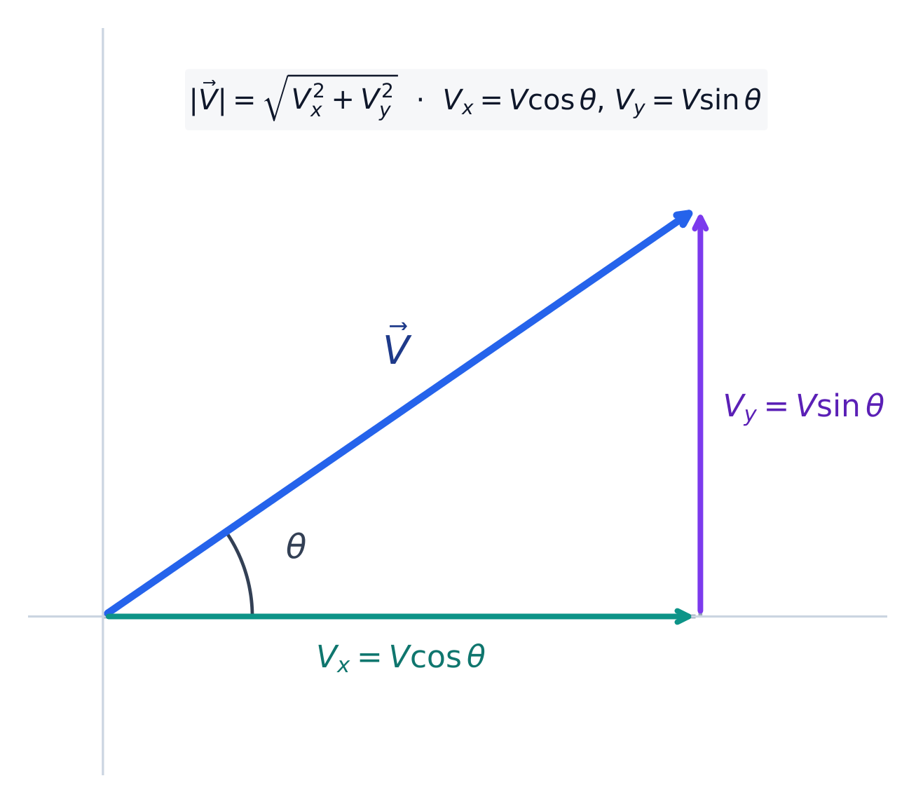
    In this calculus-based course you resolve vectors into components 分量 and add them component by component; a vector's magnitude is $\sqrt{v_x^2+v_y^2+\cdots}$. Physics C also writes vectors with unit vectors 单位矢量: $\vec{v}=v_x\hat{i}+v_y\hat{j}$, where $\hat{i}$ and $\hat{j}$ are directions of length one along $x$ and $y$ – handy because calculus can then act on each component separately.

    Español

    Cinemática describe el movimiento. Dos tipos de magnitudes:

    • Un escalar solo tiene tamaño (magnitud): distancia, rapidez, masa, tiempo.
    • Un vector tiene magnitud y dirección: desplazamiento, velocidad, aceleración, fuerza.

    En este curso basado en cálculo, resuelves los vectores en componentes y los sumas componente por componente; la magnitud de un vector es $\sqrt{v_x^2+v_y^2+\cdots}$. Física C también escribe vectores con vectores unitarios: $\vec{v}=v_x\hat{i}+v_y\hat{j}$, donde $\hat{i}$ y $\hat{j}$ son direcciones de longitud uno a lo largo de $x$ e $y$ – útil porque el cálculo puede actuar sobre cada componente por separado.

    Resolviendo un vector en sus componentes x e y
    Resolviendo un vector en sus componentes x e y
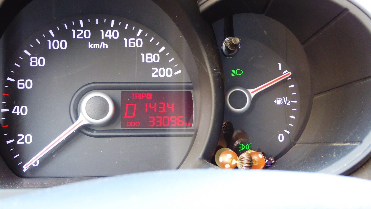
    Un velocímetro de automóvil: la rapidez es la magnitud de la velocidad — una tasa escalar de movimiento
    Un velocímetro de automóvil: la rapidez es la magnitud de la velocidad — una tasa escalar de movimiento
    Explore · ⁨Explorar⁩

    Explorar el producto escalar

    Arrastra las componentes de $\vec{A}$ y $\vec{B}$. El producto escalar $\vec{A}\cdot\vec{B}=A_xB_x+A_yB_y$ alcanza cero exactamente cuando los dos vectores son perpendiculares: la geometría detrás de $\cos\theta$.

    Vocabulary · ⁨Vocabulario⁩ Train · ⁨Entrenar⁩
    English · ⁨Inglés⁩ Chinese · ⁨Chino⁩ Pinyin
    scalar/ˈskeɪlə/ 标量 biāo liàng
    magnitude/ˈmæɡnɪtjuːd/ 大小 dà xiǎo
    vector/ˈvektə/ 矢量 shǐ liàng
    components/kəmˈpəʊnənts/ 分量 fèn liàng
    unit vectors/ˈjuːnɪt ˈvektəz/ 单位矢量 dān wèi shǐ liàng
    derivatives/dɪˈrɪvətɪvz/ 导数 dǎo shù
    average velocity/ˈævrɪdʒ vəˈlɒsɪti/ 平均速度 píng jūn sù dù
    instantaneous velocity/ˌɪnstənˈteɪnɪəs vəˈlɒsɪti/ 瞬时速度 shùn shí sù dù
    free fall/friː fɔːl/ 自由落体 zì yóu luò tǐ
    reference frame/ˈrefrəns freɪm/ 参考系 cān kǎo xì
    relative motion/ˈrelətɪv ˈməʊʃn/ 相对运动 xiāng duì yùn dòng
    projectile motion/prəˈdʒektaɪl ˈməʊʃn/ 抛体运动 pāo tǐ yùn dòng
    1.2

    Displacement, Velocity, and Acceleration · ⁨Desplazamiento, Velocidad y Aceleración⁩

    Syllabus
    English

    Learning Objective 1.2.A: Describe a change in an object's position.

    • 1.2.A.1 When using the object model, the size, shape, and internal configuration are ignored. The object may be treated as a single point with extensive properties such as mass and charge.
    • 1.2.A.2 Displacement is the change in an object's position.
      • Equation: $\Delta x = x - x_0$

    Learning Objective 1.2.B: Describe the average velocity and acceleration of an object.

    • 1.2.B.1 Averages of velocity and acceleration are calculated considering the initial and final states of an object over an interval of time.
    • 1.2.B.2 Average velocity is the displacement of an object divided by the interval of time in which that displacement occurs.
      • Equation: $\vec{v}_{\text{avg}} = \dfrac{\Delta \vec{x}}{\Delta t}$
    • 1.2.B.3 Average acceleration is the change in velocity divided by the interval of time in which that change in velocity occurs.
      • Equation: $\vec{a}_{\text{avg}} = \dfrac{\Delta \vec{v}}{\Delta t}$
    • 1.2.B.4 An object is accelerating if either the magnitude and/or direction of the object's velocity are changing.
    • 1.2.B.5 Calculating average velocity or average acceleration over a very small time interval yields a value that is very close to the instantaneous velocity or instantaneous acceleration.

    Learning Objective 1.2.C: Describe the instantaneous position, velocity, and acceleration of an object as a function of time.

    • 1.2.C.1 As the time interval used to calculate the average value of a quantity approaches zero, the average value of that quantity approaches the value of the quantity at that instant, called the instantaneous value.
      • 1.2.C.1.i Instantaneous velocity is the rate of change of the object's position, which is equal to the derivative of position with respect to time.
        • Equation: $\vec{v} = \dfrac{d\vec{r}}{dt}$
        • Equation: $v_x = \dfrac{dx}{dt}$
      • 1.2.C.1.ii Instantaneous acceleration is the rate of change of the object's velocity, which is equal to the derivative of velocity with respect to time.
        • Equation: $\vec{a} = \dfrac{d\vec{v}}{dt}$
        • Equation: $a_x = \dfrac{dv_x}{dt}$
    • 1.2.C.2 Time-dependent functions and instantaneous values of position, velocity, and acceleration can be determined using differentiation and integration.
    Español

    Objetivo de Aprendizaje 1.2.A: Describir un cambio en la posición de un objeto.

    • 1.2.A.1 Al utilizar el modelo de partícula, se ignoran el tamaño, la forma y la configuración interna del objeto. El objeto puede tratarse como un único punto con propiedades extensivas, como la masa y la carga.
    • 1.2.A.2 El desplazamiento es el cambio en la posición de un objeto.
      • Ecuación: $\Delta x = x - x_0$

    Objetivo de Aprendizaje 1.2.B: Describir la velocidad y aceleración promedio de un objeto.

    • 1.2.B.1 Los promedios de velocidad y aceleración se calculan considerando los estados inicial y final de un objeto durante un intervalo de tiempo.
    • 1.2.B.2 La velocidad promedio es el desplazamiento de un objeto dividido por el intervalo de tiempo durante el cual ocurre dicho desplazamiento.
      • Ecuación: $\vec{v}_{\text{avg}} = \dfrac{\Delta \vec{x}}{\Delta t}$
    • 1.2.B.3 La aceleración promedio es el cambio en la velocidad dividido por el intervalo de tiempo durante el cual ocurre ese cambio en la velocidad.
      • Ecuación: $\vec{a}_{\text{avg}} = \dfrac{\Delta \vec{v}}{\Delta t}$
    • 1.2.B.4 Un objeto está acelerando si cambia tanto la magnitud como/o la dirección de su velocidad.
    • 1.2.B.5 Calcular la velocidad o aceleración promedio sobre un intervalo de tiempo muy pequeño produce un valor muy cercano a la velocidad instantánea o la aceleración instantánea.

    Objetivo de Aprendizaje 1.2.C: Describir la posición, velocidad y aceleración instantáneas de un objeto en función del tiempo.

    • 1.2.C.1 A medida que el intervalo de tiempo utilizado para calcular el valor promedio de una cantidad se aproxima a cero, el valor promedio de dicha cantidad se aproxima al valor de la cantidad en ese instante, denominado valor instantáneo.
      • 1.2.C.1.i La velocidad instantánea es la tasa de cambio de la posición del objeto, lo cual es igual a la derivada de la posición con respecto al tiempo.
        • Ecuación: $\vec{v} = \dfrac{d\vec{r}}{dt}$
        • Ecuación: $v_x = \dfrac{dx}{dt}$
      • 1.2.C.1.ii La aceleración instantánea es la tasa de cambio de la velocidad del objeto, lo cual es igual a la derivada de la velocidad con respecto al tiempo.
        • Ecuación: $\vec{a} = \dfrac{d\vec{v}}{dt}$
        • Ecuación: $a_x = \dfrac{dv_x}{dt}$
    • 1.2.C.2 Las funciones dependientes del tiempo y los valores instantáneos de posición, velocidad y aceleración pueden determinarse mediante diferenciación e integración.

    Source: College Board AP Course and Exam Description · ⁨Fuente: College Board AP Course and Exam Description⁩

    English
    Projectile motion is two independent motions

    Because motion can change continuously, define the rates as derivatives 导数:

    $$v=\frac{dx}{dt},\qquad a=\frac{dv}{dt}=\frac{d^2x}{dt^2}.$$
    Reversing this, integrate to recover velocity and position:
    $$v(t)=v_0+\int_0^t a\,dt,\qquad x(t)=x_0+\int_0^t v\,dt.$$
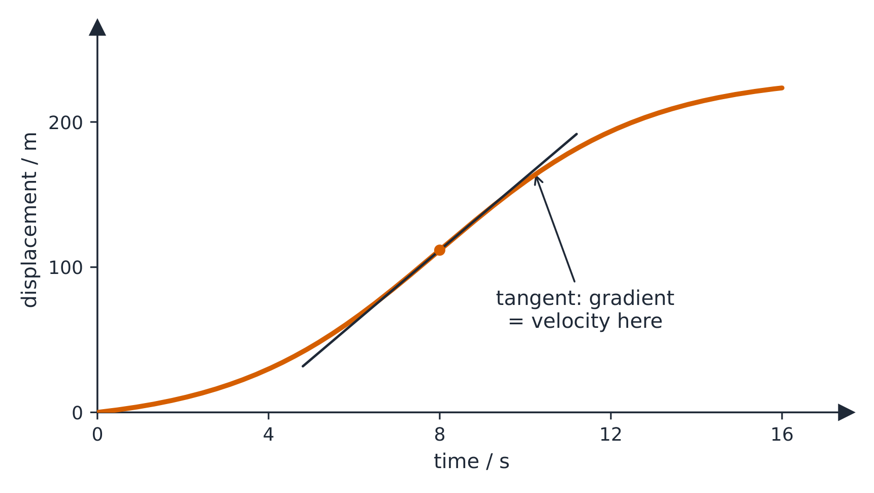
    Distinguish the average from the instantaneous: average velocity 平均速度 is $\Delta x/\Delta t$ over an interval, while instantaneous velocity 瞬时速度 is the derivative at one moment – the slope of the tangent line, and what a speedometer shows.

    For constant acceleration these give the familiar kinematic equations ($v=v_0+at$, $x=x_0+v_0t+\tfrac12at^2$, $v^2=v_0^2+2a\,\Delta x$). The most important constant-$a$ case is free fall 自由落体: near Earth's surface every object, heavy or light, accelerates downward at $g=9.8\ \text{m/s}^2$ once air resistance is negligible. When $a$ or $v$ varies with time, use the integrals directly.

    Worked example. A particle moves with $x(t)=2t^3-3t^2$ (metres). Differentiate for velocity and acceleration:

    $$v=\frac{dx}{dt}=6t^2-6t,\qquad a=\frac{dv}{dt}=12t-6.$$
    At $t=2\ \text{s}$, $v=24-12=12\ \text{m/s}$ and $a=24-6=18\ \text{m/s}^2$. This calculus link – not just the constant-$a$ formulas – is what distinguishes Physics C.

    Worked example. A particle starts from rest at the origin with $a(t)=6t$. Integrate: $v=\int 6t\,dt=3t^2$ and $x=\int 3t^2\,dt=t^3$. At $t=2\ \text{s}$, $v=12\ \text{m/s}$ and $x=8\ \text{m}$.

    Español
    El movimiento de proyectiles son dos movimientos independientes

    Dado que el movimiento puede cambiar continuamente, definimos las tasas como derivadas:

    $$v=\frac{dx}{dt},\qquad a=\frac{dv}{dt}=\frac{d^2x}{dt^2}.$$
    Invertir esto, integrar para recuperar la velocidad y la posición:
    $$v(t)=v_0+\int_0^t a\,dt,\qquad x(t)=x_0+\int_0^t v\,dt.$$
    Distingue entre promedio e instantánea: la velocidad promedio es $\Delta x/\Delta t$ sobre un intervalo, mientras que la velocidad instantánea es la derivada en un momento dado – la pendiente de la recta tangente, y lo que muestra un velocímetro.

    Para una aceleración constante, estas dan las ecuaciones cinemáticas conocidas ($v=v_0+at$, $x=x_0+v_0t+\tfrac12at^2$, $v^2=v_0^2+2a\,\Delta x$). El caso más importante de $a$ constante es la caída libre: cerca de la superficie terrestre, cada objeto, pesado o ligero, acelera hacia abajo a $g=9.8\ \text{m/s}^2$ una vez que la resistencia del aire es despreciable. Cuando $a$ o $v$ varía con el tiempo, usa las integrales directamente.

    Ejemplo resuelto. Una partícula se mueve con $x(t)=2t^3-3t^2$ (metros). Deriva para obtener velocidad y aceleración:

    $$v=\frac{dx}{dt}=6t^2-6t,\qquad a=\frac{dv}{dt}=12t-6.$$
    En $t=2\ \text{s}$, $v=24-12=12\ \text{m/s}$ y $a=24-6=18\ \text{m/s}^2$. Este vínculo con el cálculo – no solo las fórmulas de $a$ constante – es lo que distingue a Física C.

    Ejemplo resuelto. Una partícula parte del reposo en el origen con $a(t)=6t$. Integra: $v=\int 6t\,dt=3t^2$ y $x=\int 3t^2\,dt=t^3$. En $t=2\ \text{s}$, $v=12\ \text{m/s}$ y $x=8\ \text{m}$.

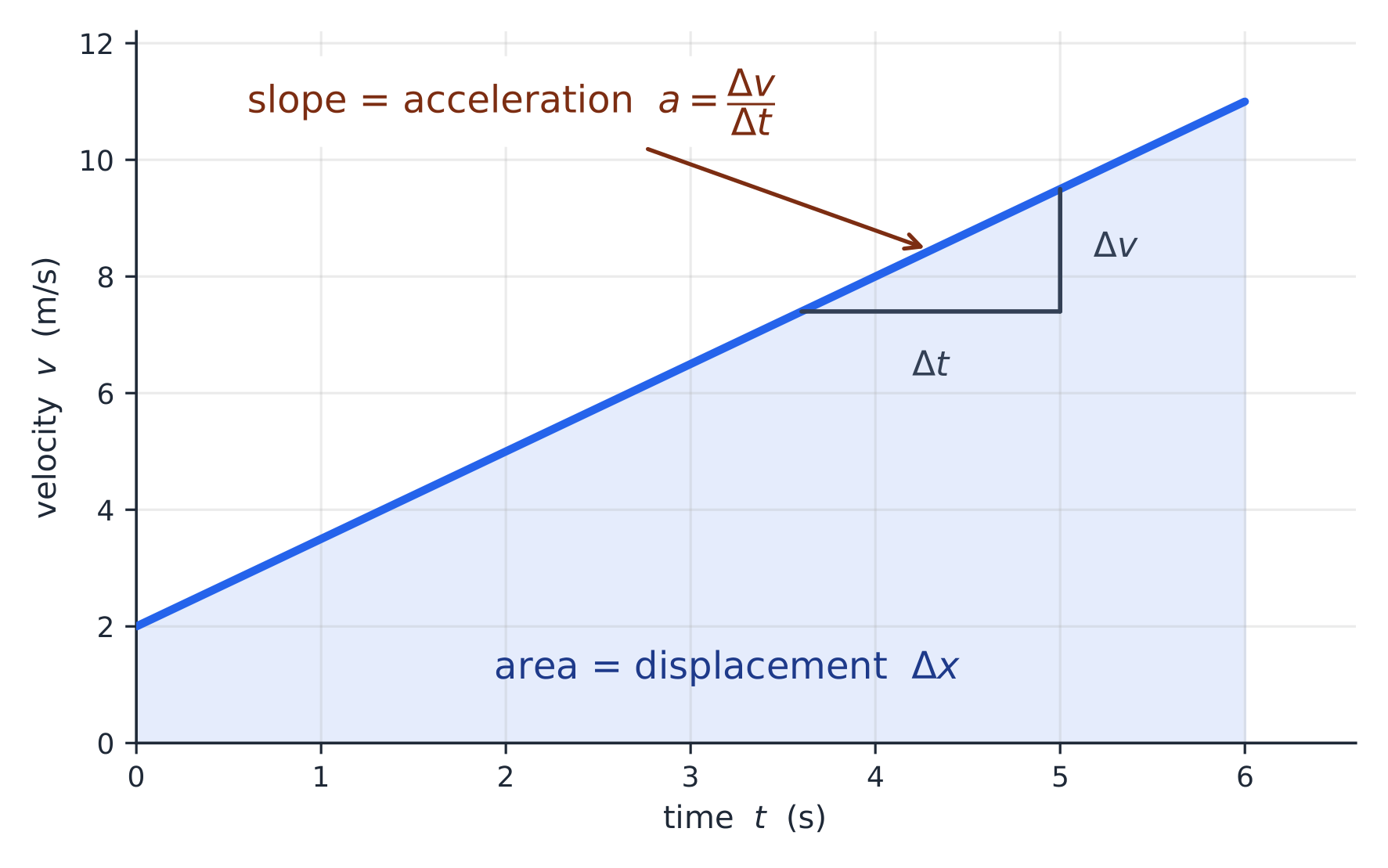
    En una gráfica de velocidad-tiempo, la pendiente es la aceleración y el área es el desplazamiento
    En una gráfica de velocidad-tiempo, la pendiente es la aceleración y el área es el desplazamiento
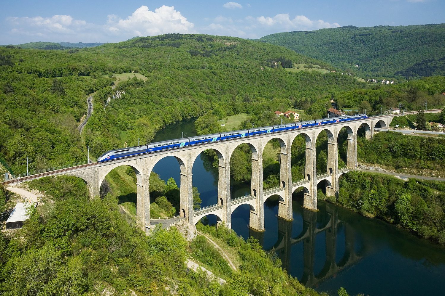
    Un tren de alta velocidad: la cinemática describe el desplazamiento, la velocidad y la aceleración a lo largo del tiempo
    Un tren de alta velocidad: la cinemática describe el desplazamiento, la velocidad y la aceleración a lo largo del tiempo
    Vocabulary · ⁨Vocabulario⁩ Train · ⁨Entrenar⁩
    English · ⁨Inglés⁩ Chinese · ⁨Chino⁩ Pinyin
    Kinematics/ˌkɪnɪˈmætɪks/ 运动学 yùn dòng xué
    1.3

    Representing Motion · ⁨Representando el Movimiento⁩

    Syllabus
    English

    Learning Objective 1.3.A: Describe the position, velocity, and acceleration of an object using representations of that object's motion.

    • 1.3.A.1 Motion can be represented by motion diagrams, figures, graphs, equations, and narrative descriptions.
    • 1.3.A.2 For constant acceleration, three kinematic equations can be used to describe instantaneous linear motion in one dimension:
      • Equation: $v_x = v_{x0} + a_x t$
      • Equation: $x = x_0 + v_{x0} t + \dfrac{1}{2} a_x t^2$
      • Equation: $v_x^2 = v_{x0}^2 + 2a_x \left( x - x_0 \right)$
      • Note: The equations above are written to indicate motion in the $x$-direction, but these equations can be used in any single dimension as appropriate.
    • 1.3.A.3 Near the surface of Earth, the vertical acceleration caused by the force of gravity is downward, constant, and has a measured value approximately equal to
      • Equation: $a_g = g \approx 10 \ \text{m/s}^2$.
    • 1.3.A.4 Graphs of position, velocity, and acceleration as functions of time can be used to find the relationships between those quantities.
      • 1.3.A.4.i An object's instantaneous velocity is the rate of change of the object's position, which is equal to the slope of a line tangent to a point on a graph of the object's position as a function of time.
        • Equation: $v_x = \dfrac{dx}{dt}$
      • 1.3.A.4.ii An object's instantaneous acceleration is the rate of change of the object's velocity, which is equal to the slope of a line tangent to a point on a graph of the object's velocity as a function of time.
        • Equation: $a_x = \dfrac{dv_x}{dt}$
      • 1.3.A.4.iii The displacement of an object during a time interval is equal to the area under the curve of a graph of the object's velocity as a function of time (i.e., the area bounded by the function and the horizontal axis for the appropriate interval).
        • Equation: $\Delta x = \displaystyle\int_{t_1}^{t_2} v_x(t) \ dt$
      • 1.3.A.4.iv The change in velocity of an object during a time interval is equal to the area under the curve of a graph of the acceleration of the object as a function of time.
        • Equation: $\Delta v_x = \displaystyle\int_{t_1}^{t_2} a_x(t) \ dt$

    Boundary statement: AP Physics C: Mechanics and AP Physics C: Electricity and Magnetism expects that for all situations in which a numerical quantity is required for g, the value $g \approx 10 \ \text{m/s}^2$ will be used. However, students will not be penalized for correctly using the more precise commonly accepted values of $g = 9.81 \ \text{m/s}^2$ or $g = 9.8 \ \text{m/s}^2$.

    Español

    Objetivo de aprendizaje 1.3.A: Describir la posición, la velocidad y la aceleración de un objeto mediante representaciones del movimiento de dicho objeto.

    • 1.3.A.1 El movimiento puede representarse mediante diagramas de movimiento, figuras, gráficos, ecuaciones y descripciones narrativas.
    • 1.3.A.2 Para una aceleración constante, se pueden utilizar tres ecuaciones cinemáticas para describir el movimiento lineal instantáneo en una dimensión:
      • Ecuación: $v_x = v_{x0} + a_x t$
      • Ecuación: $x = x_0 + v_{x0} t + \dfrac{1}{2} a_x t^2$
      • Ecuación: $v_x^2 = v_{x0}^2 + 2a_x \left( x - x_0 \right)$
      • Nota: Las ecuaciones anteriores están escritas para indicar el movimiento en la dirección $x$, pero estas ecuaciones pueden utilizarse en cualquier dimensión única según corresponda.
    • 1.3.A.3 Cerca de la superficie de la Tierra, la aceleración vertical causada por la fuerza de gravedad es hacia abajo, constante y tiene un valor medido aproximadamente igual a
      • Ecuación: $a_g = g \approx 10 \ \text{m/s}^2$.
    • 1.3.A.4 Los gráficos de posición, velocidad y aceleración como funciones del tiempo pueden utilizarse para encontrar las relaciones entre esas cantidades.
      • 1.3.A.4.i La velocidad instantánea de un objeto es la tasa de cambio de la posición del objeto, lo cual es igual a la pendiente de una línea tangente a un punto en un gráfico de la posición del objeto en función del tiempo.
        • Ecuación: $v_x = \dfrac{dx}{dt}$
      • 1.3.A.4.ii La aceleración instantánea de un objeto es la tasa de cambio de la velocidad del objeto, lo cual es igual a la pendiente de una línea tangente a un punto en un gráfico de la velocidad del objeto en función del tiempo.
        • Ecuación: $a_x = \dfrac{dv_x}{dt}$
      • 1.3.A.4.iii El desplazamiento de un objeto durante un intervalo de tiempo es igual al área bajo la curva de un gráfico de la velocidad del objeto en función del tiempo (es decir, el área delimitada por la función y el eje horizontal para el intervalo apropiado).
        • Ecuación: $\Delta x = \displaystyle\int_{t_1}^{t_2} v_x(t) \ dt$
      • 1.3.A.4.iv El cambio en la velocidad de un objeto durante un intervalo de tiempo es igual al área bajo la curva de un gráfico de la aceleración del objeto en función del tiempo.
        • Ecuación: $\Delta v_x = \displaystyle\int_{t_1}^{t_2} a_x(t) \ dt$

    Declaración de límites: AP Physics C: Mechanics y AP Physics C: Electricity and Magnetism esperan que, para todas las situaciones en las que se requiera una cantidad numérica para g, se utilice el valor $g \approx 10 \ \text{m/s}^2$. Sin embargo, no se penalizará a los estudiantes por utilizar correctamente los valores más precisos comúnmente aceptados de $g = 9.81 \ \text{m/s}^2$ o $g = 9.8 \ \text{m/s}^2$.

    Source: College Board AP Course and Exam Description · ⁨Fuente: College Board AP Course and Exam Description⁩

    English

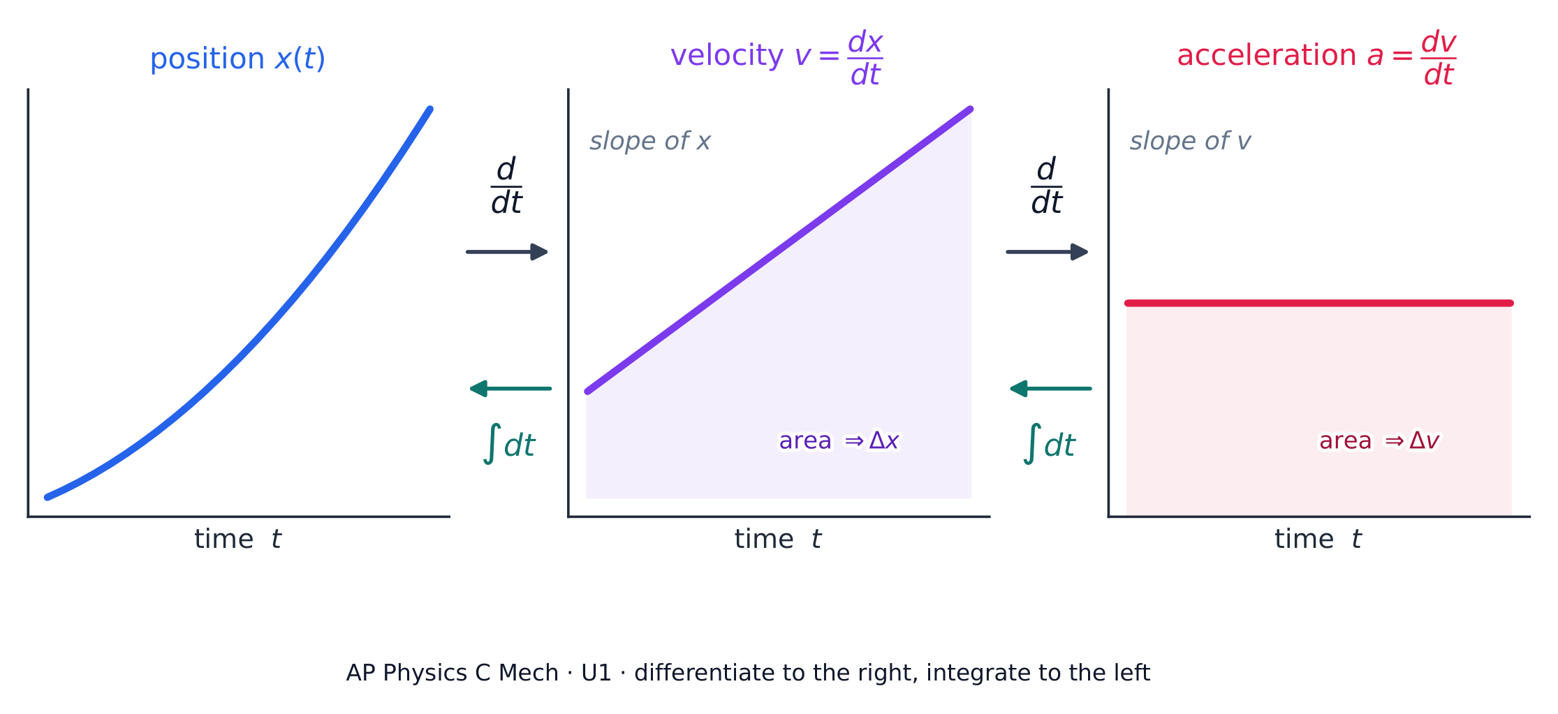
    Move fluently between description, graph, table, and equation:

    • On a position–time graph, the slope ($dx/dt$) is velocity.
    • On a velocity–time graph, the slope is acceleration and the area ($\int v\,dt$) is displacement.
    • On an acceleration–time graph, the area ($\int a\,dt$) is the change in velocity.

    Slopes are derivatives; areas are integrals – the two are inverse operations here.

    Español

    Mueve-te fluidamente entre descripción, gráfica, tabla y ecuación:

    Una gráfica de posición-tiempo: la pendiente en cualquier instante es la velocidad
    Una gráfica de posición-tiempo: la pendiente en cualquier instante es la velocidad
    • En una gráfica de posición–tiempo, la pendiente ($dx/dt$) es la velocidad.
    • En una gráfica de velocidad–tiempo, la pendiente es la aceleración y el área ($\int v\,dt$) es el desplazamiento.
    • En una gráfica de aceleración–tiempo, el área ($\int a\,dt$) es el cambio en la velocidad.

    Las pendientes son derivadas; las áreas son integrales – las dos son operaciones inversas aquí.

    Posición, velocidad y aceleración están vinculadas mediante diferenciación
    Posición, velocidad y aceleración están vinculadas mediante diferenciación
    Explore · ⁨Explorar⁩

    Explora el gráfico velocidad-tiempo

    Cambia la velocidad inicial y la aceleración. La pendiente de una línea $v$–$t$ es la aceleración $a=\tfrac{dv}{dt}$, y el área debajo es el desplazamiento $\Delta x=\int v\,dt$: la pendiente y el área son las caras gráficas de la derivada y la integral.

    1.4

    Reference Frames and Relative Motion · ⁨Marcos de Referencia y Movimiento Relativo⁩

    Syllabus
    English

    Learning Objective 1.4.A: Describe the reference frame of a given observer.

    • 1.4.A.1 The choice of reference frame will determine the direction and magnitude of quantities measured by an observer in that reference frame.

    Learning Objective 1.4.B: Describe the motion of objects as measured by observers in different inertial reference frames.

    • 1.4.B.1 Measurements from a given reference frame may be converted to measurements from another reference frame.
    • 1.4.B.2 The observed velocity of an object results from the combination of the object's velocity and the velocity of the observer's reference frame.
      • 1.4.B.2.i Combining the motion of an object and the motion of an observer in a given reference frame involves the addition or subtraction of vectors.
      • 1.4.B.2.ii The acceleration of any object is the same as measured from all inertial reference frames.

    Boundary statement: Unless otherwise stated, the frame of reference of any problem may be assumed to be inertial.

    Español

    Objetivo de aprendizaje 1.4.A: Describir el marco de referencia de un observador dado.

    • 1.4.A.1 La elección del marco de referencia determinará la dirección y la magnitud de las cantidades medidas por un observador en ese marco de referencia.

    Objetivo de aprendizaje 1.4.B: Describir el movimiento de los objetos tal como es medido por observadores en diferentes marcos de referencia inerciales.

    • 1.4.B.1 Las mediciones de un marco de referencia dado pueden convertirse en mediciones de otro marco de referencia.
    • 1.4.B.2 La velocidad observada de un objeto resulta de la combinación de la velocidad del objeto y la velocidad del marco de referencia del observador.
      • 1.4.B.2.i Combinar el movimiento de un objeto y el movimiento de un observador en un marco de referencia dado implica la suma o resta de vectores.
      • 1.4.B.2.ii La aceleración de cualquier objeto es la misma cuando se mide desde todos los marcos de referencia inerciales.

    Declaración de límite: A menos que se indique lo contrario, se puede asumir que el marco de referencia de cualquier problema es inercial.

    Source: College Board AP Course and Exam Description · ⁨Fuente: College Board AP Course and Exam Description⁩

    English

    All motion is relative to a reference frame 参考系. Combine velocities by vector addition: $\vec{v}_{A/C}=\vec{v}_{A/B}+\vec{v}_{B/C}$. This handles boats crossing rivers and passengers on moving vehicles – relative motion 相对运动 problems. Read the subscripts as a chain: "A relative to B" plus "B relative to C" gives "A relative to C".

    Worked example. A boat that moves at $4.0\ \text{m/s}$ in still water heads straight across a river flowing at $3.0\ \text{m/s}$. Relative to the ground the boat moves at $\sqrt{4.0^2+3.0^2}=5.0\ \text{m/s}$, angled downstream. If the river is $80\ \text{m}$ wide, the crossing still takes $t=\dfrac{80}{4.0}=20\ \text{s}$ – only the across-stream component crosses the river; the current just carries the boat $60\ \text{m}$ downstream.

    Español

    Todo movimiento es relativo a un marco de referencia. Combina velocidades mediante adición vectorial: $\vec{v}_{A/C}=\vec{v}_{A/B}+\vec{v}_{B/C}$. Esto maneja barcos cruzando ríos y pasajeros en vehículos en movimiento – problemas de movimiento relativo. Lee los subíndices como una cadena: "A respecto a B" más "B respecto a C" da como resultado "A respecto a C".

    Ejemplo resuelto. Un bote que se mueve a $4.0\ \text{m/s}$ en agua quieta va directamente cruzando un río que fluye a $3.0\ \text{m/s}$. Respecto al suelo, el bote se mueve a $\sqrt{4.0^2+3.0^2}=5.0\ \text{m/s}$, angulado aguas abajo. Si el río tiene $80\ \text{m}$ de ancho, el cruce todavía toma $t=\dfrac{80}{4.0}=20\ \text{s}$ – solo la componente transversal cruza el río; la corriente simplemente arrastra el bote $60\ \text{m}$ aguas abajo.

    1.5

    Motion in Two or Three Dimensions · ⁨Movimiento en Dos o Tres Dimensiones⁩

    Syllabus
    English

    Learning Objective 1.5.A: Describe the motion of an object moving in two or three dimensions.

    • 1.5.A.1 Motion in two or three dimensions can be analyzed using one-dimensional kinematic relationships if the motion is separated into components.
    • 1.5.A.2 Velocity and acceleration may be different in each dimension and may be nonuniform.
    • 1.5.A.3 Motion in one dimension may be changed without causing a change in a perpendicular dimension.
    • 1.5.A.4 Projectile motion is a special case of two-dimensional motion that has zero acceleration in one dimension and constant, nonzero acceleration in the second dimension.

    Boundary statement: AP Physics C: Mechanics only expects students to quantitatively analyze the motion of an object in two dimensions. AP Physics C: Electricity and Magnetism expects students to also qualitatively describe the motion of a particle in three dimensions.

    Español

    Objetivo de aprendizaje 1.5.A: Describir el movimiento de un objeto que se mueve en dos o tres dimensiones.

    • 1.5.A.1 El movimiento en dos o tres dimensiones puede analizarse utilizando las relaciones cinemáticas unidimensionales si el movimiento se separa en componentes.
    • 1.5.A.2 La velocidad y la aceleración pueden ser diferentes en cada dimensión y pueden no ser uniformes.
    • 1.5.A.3 El movimiento en una dimensión puede modificarse sin causar un cambio en una dimensión perpendicular.
    • 1.5.A.4 El movimiento de proyectiles es un caso especial del movimiento bidimensional que presenta aceleración nula en una dimensión y aceleración constante y distinta de cero en la segunda dimensión.

    Enunciado del límite: AP Physics C: Mechanics solo espera que los estudiantes analicen cuantitativamente el movimiento de un objeto en dos dimensiones. AP Physics C: Electricity and Magnetism espera que los estudiantes también describan cualitativamente el movimiento de una partícula en tres dimensiones.

    Source: College Board AP Course and Exam Description · ⁨Fuente: College Board AP Course and Exam Description⁩

    English

    In two or three dimensions, position is a vector $\vec{r}(t)=\langle x(t),y(t),z(t)\rangle$, and velocity and acceleration are its successive derivatives – each component handled independently.

    Worked example. $\vec{r}(t)=\big(2t^2\big)\hat{i}+\big(4t-t^3\big)\hat{j}$ (metres). Differentiating each component: $\vec{v}=4t\,\hat{i}+(4-3t^2)\,\hat{j}$ and $\vec{a}=4\,\hat{i}-6t\,\hat{j}$. At $t=1\ \text{s}$: $\vec{v}=4\hat{i}+1\hat{j}$, so the speed is $\sqrt{17}\approx4.1\ \text{m/s}$ – no new physics, just one derivative per component.

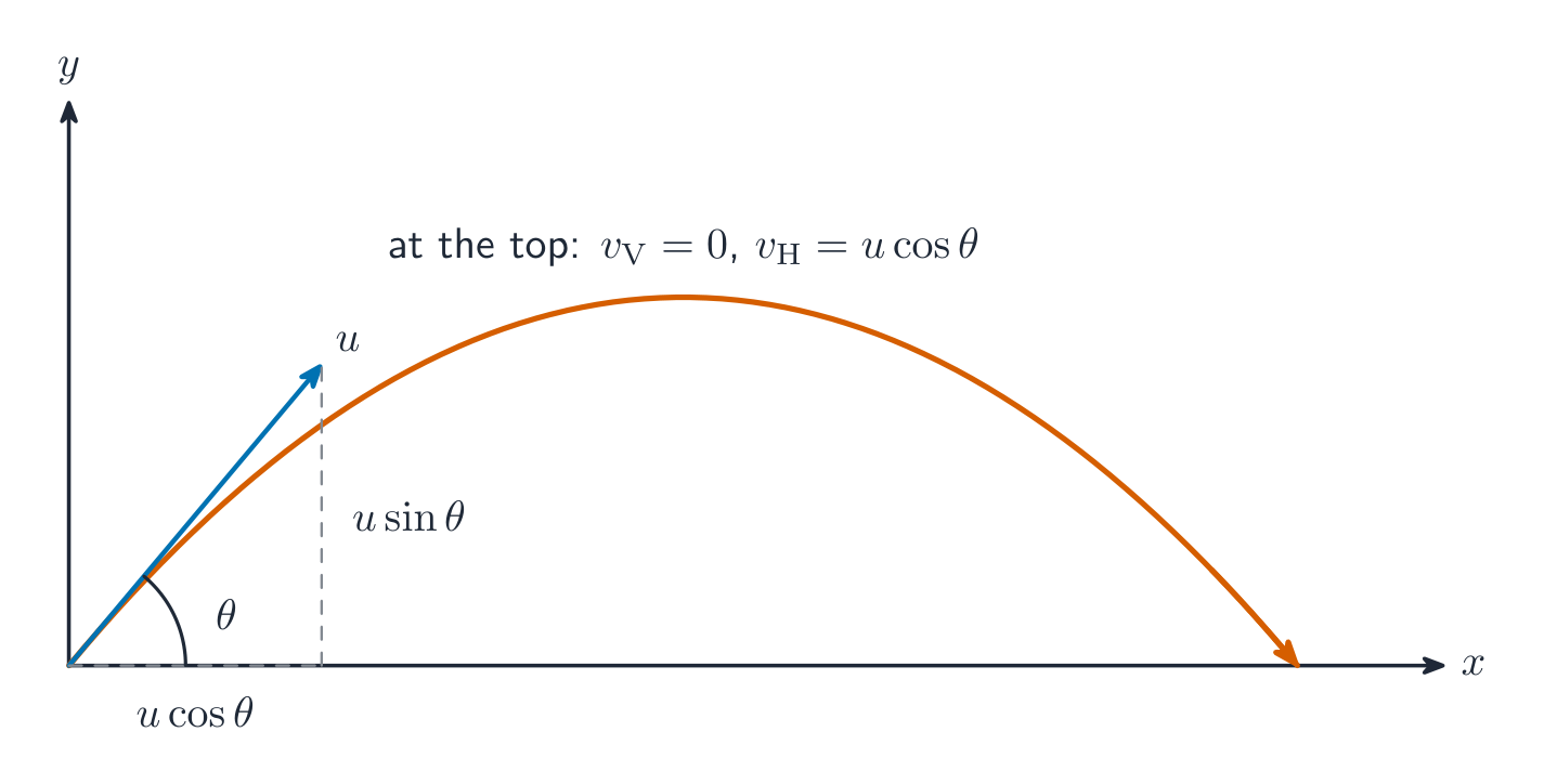
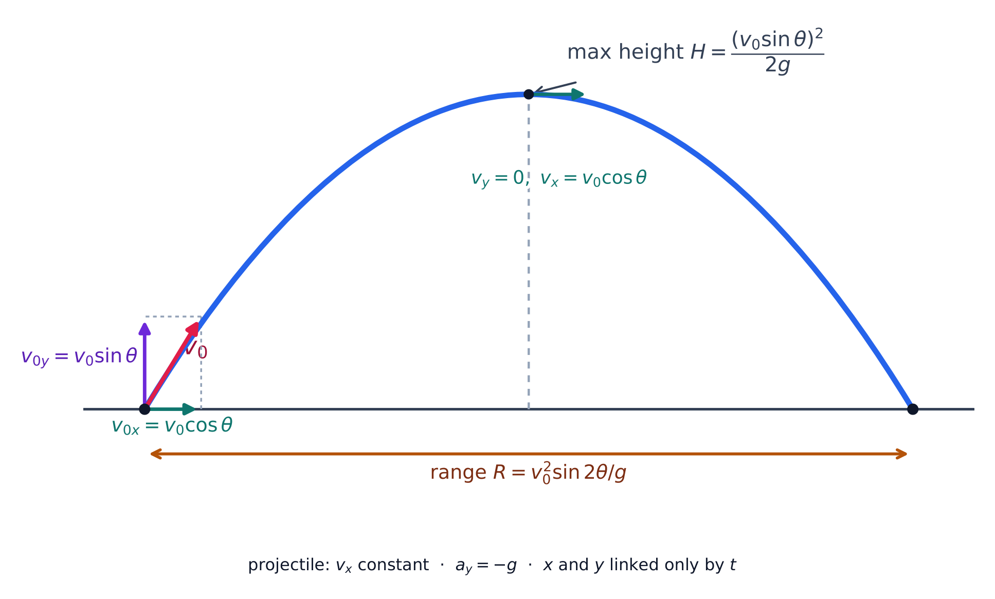
    For projectile motion 抛体运动, horizontal and vertical motions are independent, linked only by time $t$: horizontally $a_x=0$ (constant velocity), vertically $a_y=-g$. The path is a parabola. This component method extends to any two-dimensional motion where the accelerations along each axis are known.

    Worked example. A ball is launched at $20\ \text{m/s}$, $30^{\circ}$ above the horizontal ($g=9.8\ \text{m/s}^2$). The components are $v_{0x}=20\cos30^{\circ}=17.3\ \text{m/s}$ and $v_{0y}=20\sin30^{\circ}=10\ \text{m/s}$. The vertical motion sets the time: total flight $=\dfrac{2v_{0y}}{g}=\dfrac{20}{9.8}=2.0\ \text{s}$, maximum height $=\dfrac{v_{0y}^2}{2g}=5.1\ \text{m}$, and range $=v_{0x}\times2.0=35\ \text{m}$.

    Español

    En dos o tres dimensiones, la posición es un vector $\vec{r}(t)=\langle x(t),y(t),z(t)\rangle$, y la velocidad y la aceleración son sus derivadas sucesivas – cada componente se maneja de forma independiente.

    Ejemplo resuelto. $\vec{r}(t)=\big(2t^2\big)\hat{i}+\big(4t-t^3\big)\hat{j}$ (metros). Diferenciando cada componente: $\vec{v}=4t\,\hat{i}+(4-3t^2)\,\hat{j}$ y $\vec{a}=4\,\hat{i}-6t\,\hat{j}$. En $t=1\ \text{s}$: $\vec{v}=4\hat{i}+1\hat{j}$, así que la rapidez es $\sqrt{17}\approx4.1\ \text{m/s}$ – ninguna física nueva, solo una derivada por componente.

    Un proyectil lanzado en ángulo: los movimientos horizontal y vertical son independientes
    Un proyectil lanzado en ángulo: los movimientos horizontal y vertical son independientes

    Para el movimiento de proyectiles, los movimientos horizontal y vertical son independientes, vinculados solo por el tiempo $t$: horizontalmente $a_x=0$ (velocidad constante), verticalmente $a_y=-g$. La trayectoria es una parábola. Este método de componentes se extiende a cualquier movimiento bidimensional donde se conocen las aceleraciones a lo largo de cada eje.

    Ejemplo resuelto. Una pelota es lanzada a $20\ \text{m/s}$, $30^{\circ}$ sobre la horizontal ($g=9.8\ \text{m/s}^2$). Las componentes son $v_{0x}=20\cos30^{\circ}=17.3\ \text{m/s}$ y $v_{0y}=20\sin30^{\circ}=10\ \text{m/s}$. El movimiento vertical determina el tiempo: vuelo total $=\dfrac{2v_{0y}}{g}=\dfrac{20}{9.8}=2.0\ \text{s}$, altura máxima $=\dfrac{v_{0y}^2}{2g}=5.1\ \text{m}$, y alcance $=v_{0x}\times2.0=35\ \text{m}$.

    Un proyectil lanzado en ángulo: componentes de velocidad, altura máxima y alcance
    Un proyectil lanzado en ángulo: componentes de velocidad, altura máxima y alcance
    Explore · ⁨Explorar⁩

    Explorar el movimiento de proyectiles

    Lanza el proyectil, luego varía el ángulo y la velocidad. El movimiento horizontal es constante mientras la gravedad actúa solo hacia abajo; juntos trazan una parábola. Encuentra el ángulo que da el mayor alcance (alcanza su pico cerca de $45^\circ$), e intenta con la Luna.

    1.5

    Exam tips · ⁨Consejos para el examen⁩

    English
    • Resolve every vector into components before adding — never add magnitudes at an angle directly.
    • On Physics C you are expected to use calculus: velocity is $\vec v=\tfrac{d\vec r}{dt}$ and acceleration $\vec a=\tfrac{d\vec v}{dt}$; reverse with integration.
    • Carry and check units and treat direction with signs (choose a positive axis and stick to it).
    • Use the dot product for work-type quantities and the cross product for torque and angular momentum.
    • Sketch the vectors — a diagram catches sign and direction errors the algebra hides.
    Español
    • Resuelve todo vector en componentes antes de sumarlo – nunca sumes magnitudes directamente en un ángulo.
    • En Física C se espera que uses cálculo: la velocidad es $\vec v=\tfrac{d\vec r}{dt}$ y la aceleración $\vec a=\tfrac{d\vec v}{dt}$; invierte con integración.
    • Lleva y verifica las unidades y trata la dirección con signos (elige un eje positivo y mantente fiel a él).
    • Usa el producto punto para cantidades tipo trabajo y el producto cruz para torque y momento angular.
    • Haz un boceto de los vectores – un diagrama capta errores de signo y dirección que el álgebra oculta.
  • 2

    Fuerza y dinámica traslacional

    Watch lesson · ⁨Ver lección⁩
    2.1

    Systems and Center of Mass · ⁨Sistemas y centro de masa⁩

    Syllabus
    English

    Learning Objective 2.1.A: Describe the properties and interactions of a system.

    • 2.1.A.1 System properties are determined by the interactions between objects within the system.
    • 2.1.A.2 If the properties or interactions of the constituent objects within a system are not important in modeling the behavior of the macroscopic system, the system can itself be treated as a single object.
    • 2.1.A.3 Systems may allow interactions between constituent parts of the system and the environment, which may result in the transfer of energy or mass.
    • 2.1.A.4 Individual objects within a chosen system may behave differently from each other as well as from the system as a whole.
    • 2.1.A.5 The internal structure of a system affects the analysis of that system.
    • 2.1.A.6 As variables external to a system are changed, the system's substructure may change.

    Learning Objective 2.1.B: Describe the location of a system's center of mass with respect to the system's constituent parts.

    • 2.1.B.1 For objects or systems with symmetrical mass distributions, the center of mass is located on lines of symmetry.
    • 2.1.B.2 The location of a system's center of mass along a given axis can be calculated using the equation
      • Equation: $\vec{x}_{\text{cm}} = \dfrac{\sum m_i \vec{x}_i}{\sum m_i}$
    • 2.1.B.3 For a nonuniform solid that can be considered as a collection of differential masses, $dm$, the solid's center of mass can be calculated using the equation
      • Equation: $\vec{r}_{\text{cm}} = \dfrac{\int \vec{r}\, dm}{\int dm}$
      • 2.1.B.3.i The linear mass density of a rod or other linear rigid body is the derivative of the rod's mass with respect to the position of the differential mass element on the rigid body.
        • Equation: $\lambda = \dfrac{d}{d\ell} m(\ell)$
      • 2.1.B.3.ii If a function of mass density is given for a solid, the total mass can be determined by integrating the mass density over the length (one dimension), area (two dimensions), or volume (three dimensions) of the solid. For example:
        • Equation: $M_{\text{total}} = \int \rho(r)\, dV$
    • 2.1.B.4 A system can be modeled as a singular object that is located at the system's center of mass.
    Español

    Objetivo de aprendizaje 2.1.A: Describir las propiedades e interacciones de un sistema.

    • 2.1.A.1 Las propiedades del sistema se determinan por las interacciones entre los objetos dentro del sistema.
    • 2.1.A.2 Si las propiedades o interacciones de los objetos constituyentes dentro de un sistema no son importantes para modelar el comportamiento macroscópico del mismo, el sistema puede tratarse como un único objeto.
    • 2.1.A.3 Los sistemas pueden permitir interacciones entre sus partes constituyentes y el entorno, lo que puede resultar en la transferencia de energía o masa.
    • 2.1.A.4 Los objetos individuales dentro de un sistema elegido pueden comportarse de manera diferente entre sí, así como también respecto al sistema en su conjunto.
    • 2.1.A.5 La estructura interna de un sistema afecta el análisis de dicho sistema.
    • 2.1.A.6 Al cambiar variables externas a un sistema, la subestructura del mismo puede modificarse.

    Objetivo de aprendizaje 2.1.B: Describir la ubicación del centro de masa de un sistema con respecto a sus partes constituyentes.

    • 2.1.B.1 Para objetos o sistemas con distribuciones de masa simétricas, el centro de masa se encuentra sobre líneas de simetría.
    • 2.1.B.2 La ubicación del centro de masa de un sistema a lo largo de un eje dado se puede calcular mediante la ecuación:
      • Ecuación: $\vec{x}_{\text{cm}} = \dfrac{\sum m_i \vec{x}_i}{\sum m_i}$
    • 2.1.B.3 Para un sólido no uniforme que puede considerarse como una colección de masas diferenciales $dm$, el centro de masa del sólido se puede calcular mediante la ecuación:
      • Ecuación: $\vec{r}_{\text{cm}} = \dfrac{\int \vec{r}\, dm}{\int dm}$
      • 2.1.B.3.i La densidad lineal de masa de una barra u otro cuerpo rígido lineal es la derivada de la masa de la barra con respecto a la posición del elemento de masa diferencial sobre el cuerpo rígido.
        • Ecuación: $\lambda = \dfrac{d}{d\ell} m(\ell)$
      • 2.1.B.3.ii Si se proporciona una función de densidad de masa para un sólido, la masa total se puede determinar integrando la densidad de masa a lo largo de la longitud (una dimensión), área (dos dimensiones) o volumen (tres dimensiones) del sólido. Por ejemplo:
        • Ecuación: $M_{\text{total}} = \int \rho(r)\, dV$
    • 2.1.B.4 Un sistema puede modelarse como un objeto singular ubicado en el centro de masa del sistema.

    Source: College Board AP Course and Exam Description · ⁨Fuente: College Board AP Course and Exam Description⁩

    English

    A system 系统 is the object or objects you analyze, treated as a point at its center of mass 质心. For a set of masses, $x_{\text{cm}}=\dfrac{\sum m_i x_i}{\sum m_i}$; for a continuous body, $x_{\text{cm}}=\dfrac{1}{M}\int x\,dm$. Only external forces move the center of mass.

    Español

    Un sistema 系统是分析的对象或物体组,被视为位于其 centro de masa 质心的一个 punto. Para un conjunto de masas, $x_{\text{cm}}=\dfrac{\sum m_i x_i}{\sum m_i}$; para un cuerpo continuo, $x_{\text{cm}}=\dfrac{1}{M}\int x\,dm$. Solo las fuerzas externas 外部移动 el centro de masa.

    2.2

    Forces and Free-Body Diagrams · ⁨Fuerzas y diagramas de cuerpo libre⁩

    Syllabus
    English

    Learning Objective 2.2.A: Describe a force as an interaction between two objects or systems

    • 2.2.A.1 Forces are vector quantities that describe the interactions between objects or systems.
      • 2.2.A.1.i A force exerted on an object or system is always due to the interaction of that object or system with another object or system.
      • 2.2.A.1.ii An object or system cannot exert a net force on itself.
    • 2.2.A.2 Contact forces describe the interaction of an object or system touching another object or system and are macroscopic effects of interatomic electric forces.

    Learning Objective 2.2.B: Describe the forces exerted on an object or system using a free-body diagram.

    • 2.2.B.1 Free-body diagrams are useful tools for visualizing forces being exerted on a single object or system and for determining the equations that represent a physical situation.
    • 2.2.B.2 The free-body diagram of an object or system shows each of the forces exerted on the object or system by the environment.
    • 2.2.B.3 Forces exerted on an object or system are represented as vectors originating from the representation of the center of mass, such as a dot. A system is treated as though all of its mass is located at the center of mass.
    • 2.2.B.4 A coordinate system with one axis parallel to the direction of acceleration of the object or system simplifies the translation from free-body diagram to algebraic representation. For example, in a free-body diagram of an object on an inclined plane, it is useful to set one axis parallel to the surface of the incline.

    Boundary statement: AP Physics C: Mechanics and AP Physics C: Electricity and Magnetism only expect students to depict the forces exerted on objects, not the force components on free-body diagrams. On the AP Physics exams, individual forces represented on a free-body diagram must be drawn as individual straight arrows, originating on the dot and pointing in the direction of the force. Individual forces that are in the same direction must be drawn side by side, not overlapping.

    Español

    Objetivo de aprendizaje 2.2.A: Describir una fuerza como una interacción entre dos objetos o sistemas

    • 2.2.A.1 Las fuerzas son cantidades vectoriales que describen las interacciones entre objetos o sistemas.
      • 2.2.A.1.i Una fuerza ejercida sobre un objeto o sistema se debe siempre a la interacción de ese objeto o sistema con otro objeto o sistema.
      • 2.2.A.1.ii Un objeto o sistema no puede ejercer una fuerza neta sobre sí mismo.
    • 2.2.A.2 Las fuerzas de contacto describen la interacción de un objeto o sistema que toca otro objeto o sistema, y son efectos macroscópicos de las fuerzas eléctricas interatómicas.

    Objetivo de aprendizaje 2.2.B: Describir las fuerzas ejercidas sobre un objeto o sistema mediante un diagrama de cuerpo libre.

    • 2.2.B.1 Los diagramas de cuerpo libre son herramientas útiles para visualizar las fuerzas que actúan sobre un solo objeto o sistema y para determinar las ecuaciones que representan una situación física.
    • 2.2.B.2 El diagrama de cuerpo libre de un objeto o sistema muestra cada una de las fuerzas que el entorno ejerce sobre el objeto o sistema.
    • 2.2.B.3 Las fuerzas ejercidas sobre un objeto o sistema se representan como vectores que parten de la representación del centro de masa, como un punto. Un sistema se trata como si toda su masa estuviera ubicada en su centro de masa.
    • 2.2.B.4 Un sistema de coordenadas con un eje paralelo a la dirección de aceleración del objeto o sistema simplifica la transición del diagrama de cuerpo libre a la representación algebraica. Por ejemplo, en un diagrama de cuerpo libre de un objeto sobre un plano inclinado, es útil establecer un eje paralelo a la superficie del plano.

    Declaración de límites: AP Physics C: Mechanics y AP Physics C: Electricity and Magnetism solo esperan que los estudiantes representen las fuerzas ejercidas sobre los objetos, no las componentes de fuerza en los diagramas de cuerpo libre. En los exámenes de AP Physics, las fuerzas individuales representadas en un diagrama de cuerpo libre deben dibujarse como flechas rectas individuales, originándose en el punto y apuntando en la dirección de la fuerza. Las fuerzas individuales que están en la misma dirección deben dibujarse una al lado de la otra, sin superponerse.

    Source: College Board AP Course and Exam Description · ⁨Fuente: College Board AP Course and Exam Description⁩

    English

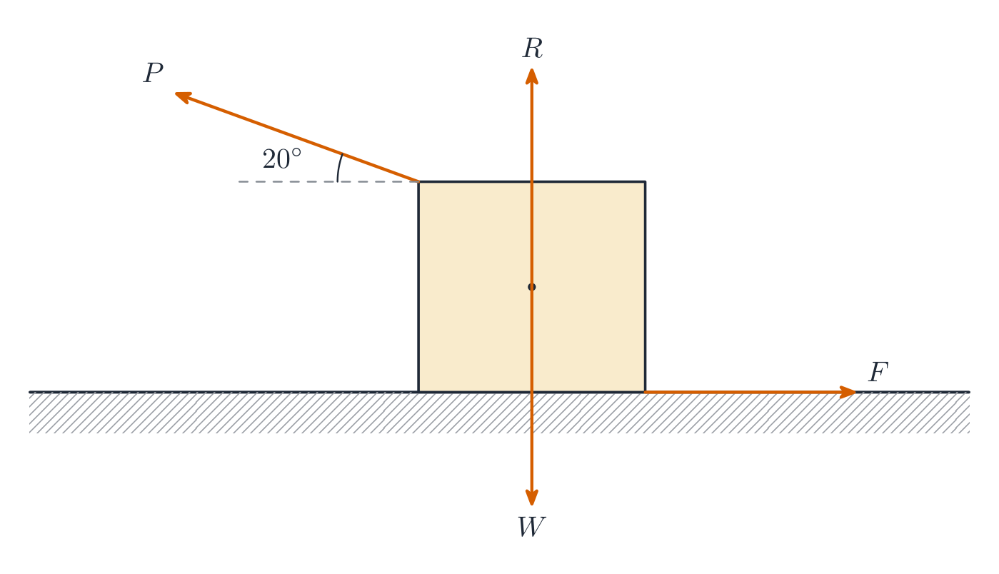
    A force 力 is a push or pull (a vector, in newtons). A free-body diagram 受力图 draws one object with an arrow for every force on it – weight, normal, tension, friction, applied, drag. Draw it first; it sets up every dynamics equation.

    Español

    Una fuerza 力 es un empuje o jalón (un vector, en newtons). Un diagrama de cuerpo libre 受力图 dibuja un solo objeto con una flecha para cada fuerza que actúa sobre él – peso, normal, tensión, fricción, aplicada, resistencia. Dibújalo primero; esto establece todas las ecuaciones de dinámica.

    Un diagrama de cuerpo libre muestra cada fuerza que actúa sobre un solo objeto
    Un diagrama de cuerpo libre muestra todas las fuerzas actuando sobre un solo objeto
    Explore · ⁨Explorar⁩

    Equilibrar las fuerzas en un diagrama de cuerpo libre

    Un diagrama de cuerpo libre muestra cada fuerza sobre un objeto como una flecha. El objeto acelera solo si las fuerzas no se cancelan; la fuerza neta establece $a=F/m$.

    Vocabulary · ⁨Vocabulario⁩ Train · ⁨Entrenar⁩
    English · ⁨Inglés⁩ Chinese · ⁨Chino⁩ Pinyin
    free-body diagram/friː ˈbɒdi ˈdaɪəɡræm/ 受力图 shòu lì tú
    Newton's third law/ˈnjuːtnz θɜːd lɔː/ 牛顿第三定律 niú dùn dì sān dìng lǜ
    inertia/ɪˈnɜːʃə/ 惯性 guàn xìng
    net force/net fɔːs/ 合力 hé lì
    translational equilibrium/trænˈsleɪʃənl ˌiːkwɪˈlɪbrɪəm/ 平动平衡 píng dòng píng héng
    differential equation/ˌdɪfəˈrenʃl ɪˈkweɪʒn/ 微分方程 wēi fēn fāng chéng
    incline/ɪnˈklaɪn/ 斜面 xié miàn
    tension/ˈtenʃn/ 张力 zhāng lì
    Newton's law of gravitation/ˈnjuːtnz lɔː ɒv ˌɡrævɪˈteɪʃn/ 万有引力定律 wàn yǒu yǐn lì dìng lǜ
    Friction/ˈfrɪkʃn/ 摩擦力 mó cā lì
    kinetic/kɪˈnetɪk/ 动摩擦 dòng mó cā
    static/ˈstætɪk/ 静摩擦 jìng mó cā
    normal force/ˈnɔːml fɔːs/ 法向力 fǎ xiàng lì
    2.3

    Newton's Third Law · ⁨Tercera ley de Newton⁩

    Syllabus
    English

    Learning Objective 2.3.A: Describe the interaction of two objects or systems using Newton's third law and a representation of paired forces exerted on each object or system.

    • 2.3.A.1 Newton's third law describes the interaction of two objects or systems in terms of the paired forces that each exerts on the other.
      • Equation: $\vec{F}_{\text{A on B}} = -\vec{F}_{\text{B on A}}$
    • 2.3.A.2 Interactions between objects within a system (internal forces) do not influence the motion of a system's center of mass.
    • 2.3.A.3 Tension is the macroscopic net result of forces that infinitesimal segments of a string, cable, chain, or similar system exert on each other in response to an external force.
      • 2.3.A.3.i An ideal string has negligible mass and does not stretch when under tension.
      • 2.3.A.3.ii The tension in an ideal string is the same at all points within the string.
      • 2.3.A.3.iii In a string with nonnegligible mass, tension may not be the same at all points within the string.
      • 2.3.A.3.iv An ideal pulley is a pulley that has negligible mass and rotates about an axle through its center of mass with negligible friction.
    Español

    Objetivo de aprendizaje 2.3.A: Describir la interacción entre dos objetos o sistemas mediante la tercera ley de Newton y una representación de las fuerzas aparejadas que cada objeto o sistema ejerce sobre el otro.

    • 2.3.A.1 La tercera ley de Newton describe la interacción entre dos objetos o sistemas en términos de las fuerzas aparejadas que cada uno ejerce sobre el otro.
      • Ecuación: $\vec{F}_{\text{A on B}} = -\vec{F}_{\text{B on A}}$
    • 2.3.A.2 Las interacciones entre objetos dentro de un sistema (fuerzas internas) no influyen en el movimiento del centro de masa de un sistema.
    • 2.3.A.3 La tensión es el resultado neto macroscópico de las fuerzas que los segmentos infinitesimales de una cuerda, cable, cadena o sistema similar ejercen entre sí en respuesta a una fuerza externa.
      • 2.3.A.3.i Una cuerda ideal tiene masa despreciable y no se estira cuando está sometida a tensión.
      • 2.3.A.3.ii La tensión en una cuerda ideal es la misma en todos los puntos de la cuerda.
      • 2.3.A.3.iii En una cuerda con masa no despreciable, la tensión puede no ser la misma en todos los puntos de la cuerda.
      • 2.3.A.3.iv Una polea ideal es una polea que tiene masa despreciable y gira alrededor de un eje que pasa por su centro de masa con fricción despreciable.

    Source: College Board AP Course and Exam Description · ⁨Fuente: College Board AP Course and Exam Description⁩

    English

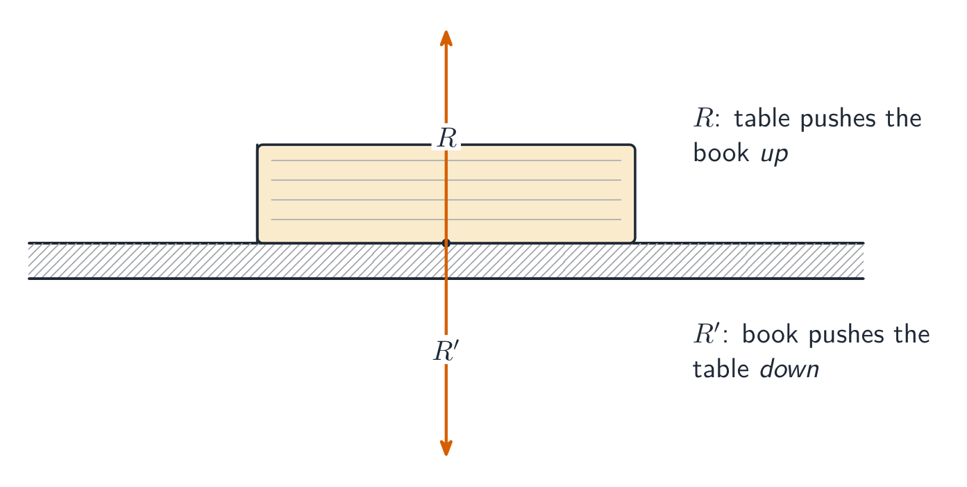
    Newton's third law 牛顿第三定律: A pushes B, B pushes back equally and oppositely. The pair acts on different objects, so it never cancels within one free-body diagram.

    Español

    Tercera ley de Newton 牛顿第三定律: A empuja a B, y B empuja de vuelta con igual magnitud y dirección opuesta. El par actúa sobre objetos diferentes, por lo que nunca se cancela dentro de un solo diagrama de cuerpo libre.

    Un par de la tercera ley de Newton: fuerzas iguales y opuestas sobre dos objetos diferentes
    Un par de la tercera ley de Newton: fuerzas iguales y opuestas sobre dos objetos diferentes
    2.4

    Newton's First Law · ⁨Primera ley de Newton⁩

    Syllabus
    English

    Learning Objective 2.4.A: Describe the conditions under which a system's velocity remains constant.

    • 2.4.A.1 The net force on a system is the vector sum of all forces exerted on the system.
    • 2.4.A.2 Translational equilibrium is the configuration of forces such that the net force exerted on a system is zero.
      • Derived equation: $\sum \vec{F}_i = 0$
    • 2.4.A.3 Newton's first law states that if the net force exerted on a system is zero, the velocity of that system will remain constant.
    • 2.4.A.4 Forces may be balanced in one dimension but unbalanced in another. The system's velocity will change only in the direction of the unbalanced force.
    • 2.4.A.5 An inertial reference frame is one from which an observer would verify Newton's first law of motion.
    Español

    Objetivo de aprendizaje 2.4.A: Describir las condiciones bajo las cuales la velocidad de un sistema permanece constante.

    • 2.4.A.1 La fuerza neta sobre un sistema es la suma vectorial de todas las fuerzas que actúan sobre el sistema.
    • 2.4.A.2 El equilibrio traslacional es la configuración de fuerzas tal que la fuerza neta ejercida sobre un sistema es cero.
      • Ecuación derivada: $\sum \vec{F}_i = 0$
    • 2.4.A.3 La primera ley de Newton establece que si la fuerza neta ejercida sobre un sistema es cero, la velocidad de dicho sistema permanecerá constante.
    • 2.4.A.4 Las fuerzas pueden estar equilibradas en una dimensión pero desequilibradas en otra. La velocidad del sistema cambiará únicamente en la dirección de la fuerza no equilibrada.
    • 2.4.A.5 Un marco de referencia inercial es aquel desde el cual un observador podría verificar la primera ley del movimiento de Newton.

    Source: College Board AP Course and Exam Description · ⁨Fuente: College Board AP Course and Exam Description⁩

    English

    Newton's first law (inertia 惯性): with zero net force 合力, velocity stays constant – the object is in translational equilibrium 平动平衡.

    Español

    Primera ley de Newton (inercia 惯性): con una fuerza neta 合力 cero, la velocidad permanece constante – el objeto está en equilibrio traslacional 平动平衡.

    2.5

    Newton's Second Law · ⁨Segunda ley de Newton⁩

    Syllabus
    English

    Learning Objective 2.5.A: Describe the conditions under which a system's velocity changes.

    • 2.5.A.1 Unbalanced forces are a configuration of forces such that the net force exerted on a system is not equal to zero.
    • 2.5.A.2 Newton's second law of motion states that the acceleration of a system's center of mass has a magnitude proportional to the magnitude of the net force exerted on the system and is in the same direction as that net force.
      • Equation: $\vec{a}_{\text{sys}} = \dfrac{\sum \vec{F}}{m_{\text{sys}}} = \dfrac{\vec{F}_{\text{net}}}{m_{\text{sys}}}$
    • 2.5.A.3 The velocity of a system's center of mass will only change if a nonzero net external force is exerted on that system.
    Español

    Objetivo de aprendizaje 2.5.A: Describir las condiciones bajo las cuales cambia la velocidad de un sistema.

    • 2.5.A.1 Las fuerzas no equilibradas son una configuración de fuerzas tal que la fuerza neta ejercida sobre un sistema no es igual a cero.
    • 2.5.A.2 La segunda ley del movimiento de Newton establece que la aceleración del centro de masa de un sistema tiene una magnitud proporcional a la magnitud de la fuerza neta ejercida sobre el sistema y se encuentra en la misma dirección que dicha fuerza neta.
      • Ecuación: $\vec{a}_{\text{sys}} = \dfrac{\sum \vec{F}}{m_{\text{sys}}} = \dfrac{\vec{F}_{\text{net}}}{m_{\text{sys}}}$
    • 2.5.A.3 La velocidad del centro de masa de un sistema solo cambiará si se ejerce sobre ese sistema una fuerza externa neta distinta de cero.

    Source: College Board AP Course and Exam Description · ⁨Fuente: College Board AP Course and Exam Description⁩

    English

    The general form uses momentum:

    $$\sum\vec{F}=\frac{d\vec{p}}{dt}=m\vec{a}\ \ (\text{for constant mass}).$$
    Apply it one axis at a time. When forces depend on velocity or position, this becomes a differential equation 微分方程 to solve.

    Worked example. A $2.0\ \text{kg}$ block slides down a frictionless incline 斜面 at $30^{\circ}$. Only the along-ramp component of gravity drives it, so $a=g\sin30^{\circ}=9.8(0.5)=4.9\ \text{m/s}^2$, independent of the mass.

    Worked example (two bodies). A $6.0\ \text{kg}$ cart on a frictionless table is pulled by a string over a light pulley to a hanging $2.0\ \text{kg}$ mass. Treat the pair as one system: only the hanging weight drives it, so $a=\dfrac{2.0(9.8)}{8.0}=2.45\ \text{m/s}^2$. Then isolate the cart alone to find the string tension 张力: $T=6.0(2.45)\approx15\ \text{N}$. System first for $a$, single body for internal forces – that two-step is the standard pattern.

    Español

    La forma general utiliza el momento lineal:

    $$\sum\vec{F}=\frac{d\vec{p}}{dt}=m\vec{a}\ \ (\text{for constant mass}).$$
    Aplica esta ley un eje a la vez. Cuando las fuerzas dependen de la velocidad o posición, esto se convierte en una ecuación diferencial 微分方程 para resolver.

    Ejemplo resuelto. Un bloque de $2.0\ \text{kg}$ desliza hacia abajo por un plano inclinado 斜面 sin fricción a $30^{\circ}$. Solo la componente del gravedad paralela al plano lo impulsa, así que $a=g\sin30^{\circ}=9.8(0.5)=4.9\ \text{m/s}^2$, independiente de la masa.

    Ejemplo resuelto (dos cuerpos). Un carrito de $6.0\ \text{kg}$ sobre una mesa sin fricción es jalado por una cuerda a través de una polea ligera hacia una masa colgante de $2.0\ \text{kg}$. Trata el par como un solo sistema: solo el peso colgante lo impulsa, así que $a=\dfrac{2.0(9.8)}{8.0}=2.45\ \text{m/s}^2$. Luego aísla el carrito solo para encontrar la tensión 张力 de la cuerda: $T=6.0(2.45)\approx15\ \text{N}$. Sistema primero para $a$, cuerpo único para fuerzas internas – ese patrón de dos pasos es el estándar.

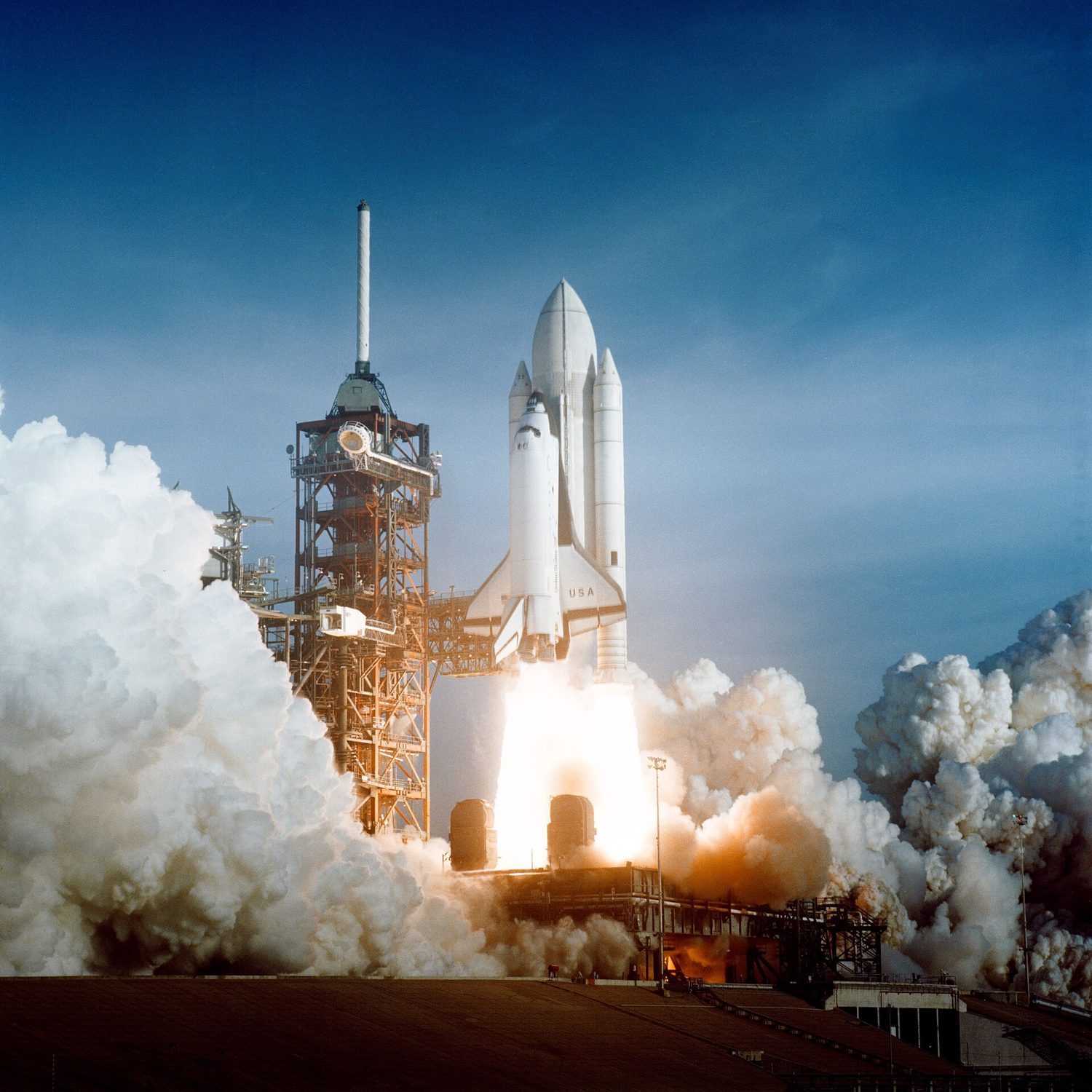
    Un lanzamiento de cohete: la fuerza neta cambia el momento — F_neta = ma para la dinámica traslacional
    Un lanzamiento de cohete: la fuerza neta cambia el momento — F_net = ma para la dinámica traslacional
    Vocabulary · ⁨Vocabulario⁩ Train · ⁨Entrenar⁩
    English · ⁨Inglés⁩ Chinese · ⁨Chino⁩ Pinyin
    system/ˈsɪstəm/ 系统 xì tǒng
    center of mass/ˈsentə ɒv mæs/ 质心 zhì xīn
    force/fɔːs/ 力 lì
    2.6

    Gravitational Force · ⁨Fuerza gravitacional⁩

    Syllabus
    English

    Learning Objective 2.6.A: Describe the gravitational interaction between two objects or systems with mass.

    • 2.6.A.1 Newton's law of universal gravitation describes the gravitational force between two objects or systems as directly proportional to each of their masses and inversely proportional to the square of the distance between the systems' centers of mass.
      • Equation: $\left| \vec{F}_g \right| = G \dfrac{m_1 m_2}{r^2}$
      • 2.6.A.1.i The gravitational force is attractive.
      • 2.6.A.1.ii The gravitational force is always exerted along the line connecting the center of mass of the two interacting systems.
      • 2.6.A.1.iii The gravitational force on a system can be considered to be exerted on the system's center of mass.
    • 2.6.A.2 A field models the effects of a noncontact force exerted on an object at various positions in space.
      • 2.6.A.2.i The magnitude of the gravitational field created by a system of mass $M$ at a point in space is equal to the ratio of the gravitational force exerted by the system on a test object of mass $m$ to the mass of the test object.
        • Derived equation: $\left| \vec{g} \right| = \dfrac{\left| \vec{F}_g \right|}{m} = G \dfrac{M}{r^2}$
      • 2.6.A.2.ii If the gravitational force is the only force exerted on an object, the observed acceleration of the object (in $\text{m/s}^2$) is numerically equal to the magnitude of the gravitational field strength (in $\text{N/kg}$) at that location.
    • 2.6.A.3 The gravitational force exerted by an astronomical body on a relatively small nearby object is called weight.
      • Derived equation: $\text{Weight} = F_g = mg$

    Learning Objective 2.6.B: Describe situations in which the gravitational force can be considered constant.

    • 2.6.B.1 If the gravitational force between two systems' centers of mass has a negligible change as the relative position of the two systems changes, the gravitational force can be considered constant at all points between the initial and final positions of the systems.
    • 2.6.B.2 Near the surface of Earth, the strength of the gravitational field is
      • Equation: $g \approx 10\ \text{N/kg}$

    Learning Objective 2.6.C: Describe the conditions under which the magnitude of a system's apparent weight is different from the magnitude of the gravitational force exerted on that system.

    • 2.6.C.1 The magnitude of the apparent weight of a system is the magnitude of the normal force exerted on the system.
    • 2.6.C.2 If the system is accelerating, the apparent weight of the system is not equal to the magnitude of the gravitational force exerted on the system.
    • 2.6.C.3 A system appears weightless when there are no forces exerted on the system or when the force of gravity is the only force exerted on the system.
    • 2.6.C.4 The equivalence principle states that an observer in a noninertial reference frame is unable to distinguish between an object's apparent weight and the gravitational force exerted on the object by a gravitational field.

    Learning Objective 2.6.D: Describe inertial and gravitational mass.

    • 2.6.D.1 Objects have inertial mass, or inertia, a property that determines how much an object's motion resists changes when interacting with another object.
    • 2.6.D.2 Gravitational mass is related to the force of attraction between two systems with mass.
    • 2.6.D.3 Inertial mass and gravitational mass have been experimentally verified to be equivalent.

    Learning Objective 2.6.E: Describe the gravitational force exerted on an object by a uniform spherical distribution of mass.

    • 2.6.E.1 The net gravitational force exerted on an object by a uniform spherical distribution of mass is the sum of the individual forces from small differential masses that comprise the distribution.
    • 2.6.E.2 Newton's shell theorem describes the net gravitational force exerted on an object by a uniform spherical shell of mass.
      • 2.6.E.2.i The net gravitational force exerted on an object inside a thin spherical shell is zero.
      • 2.6.E.2.ii The net gravitational force exerted on an object outside a thin spherical shell can be determined by treating the shell as a single massive object located at the center of the shell.
      • 2.6.E.2.iii An object inside a sphere of uniform density experiences a net gravitational force from only a partial mass of the sphere.
      • 2.6.E.2.iv The partial mass of a sphere that contributes to the net gravitational force exerted on an object within that sphere is the portion of the sphere's mass located a distance less than or equal to the object's distance from the center of the sphere and can be calculated using the density of the sphere.
        • Derived equation: $m_{\text{partial}} = \rho \dfrac{4}{3} \pi \left( r_{\text{partial}} \right)^3$
    • 2.6.E.3 The gravitational force exerted on an object within a uniform sphere can be shown to be proportional to the object's distance from the sphere's center.
      • Derived equation: $F_{g,\text{partial}} = -k r_{\text{partial}}$

    Boundary statement: AP Physics C: Mechanics does not expect students to mathematically prove or derive Newton's shell theorem.

    Español

    Objetivo de aprendizaje 2.6.A: Describir la interacción gravitatoria entre dos objetos o sistemas con masa.

    • 2.6.A.1 La ley de gravitación universal de Newton describe la fuerza gravitatoria entre dos objetos o sistemas como directamente proporcional a cada una de sus masas e inversamente proporcional al cuadrado de la distancia entre los centros de masa de los sistemas.
      • Ecuación: $\left| \vec{F}_g \right| = G \dfrac{m_1 m_2}{r^2}$
      • 2.6.A.1.i La fuerza gravitatoria es atractiva.
      • 2.6.A.1.ii La fuerza gravitatoria siempre se ejerce a lo largo de la línea que conecta el centro de masa de los dos sistemas interactuantes.
      • 2.6.A.1.iii La fuerza gravitatoria sobre un sistema puede considerarse ejercida sobre el centro de masa del sistema.
    • 2.6.A.2 Un campo modela los efectos de una fuerza no contactante ejercida sobre un objeto en varias posiciones en el espacio.
      • 2.6.A.2.i La magnitud del campo gravitatorio creado por un sistema de masa $M$ en un punto del espacio es igual a la razón entre la fuerza gravitatoria ejercida por el sistema sobre un objeto de prueba de masa $m$ y la masa del objeto de prueba.
        • Ecuación derivada: $\left| \vec{g} \right| = \dfrac{\left| \vec{F}_g \right|}{m} = G \dfrac{M}{r^2}$
      • 2.6.A.2.ii Si la fuerza gravitatoria es la única fuerza ejercida sobre un objeto, la aceleración observada del objeto (en $\text{m/s}^2$) es numéricamente igual a la magnitud de la intensidad del campo gravitatorio (en $\text{N/kg}$) en esa ubicación.
    • 2.6.A.3 La fuerza gravitatoria ejercida por un cuerpo astronómico sobre un objeto cercano relativamente pequeño se denomina peso.
      • Ecuación derivada: $\text{Weight} = F_g = mg$

    Objetivo de aprendizaje 2.6.B: Describir situaciones en las que la fuerza gravitatoria puede considerarse constante.

    • 2.6.B.1 Si la fuerza gravitatoria entre los centros de masa de dos sistemas tiene un cambio despreciable a medida que cambia la posición relativa de los dos sistemas, la fuerza gravitatoria puede considerarse constante en todos los puntos entre las posiciones inicial y final de los sistemas.
    • 2.6.B.2 Cerca de la superficie de la Tierra, la intensidad del campo gravitatorio es
      • Ecuación: $g \approx 10\ \text{N/kg}$

    Objetivo de aprendizaje 2.6.C: Describir las condiciones bajo las cuales la magnitud del peso aparente de un sistema es diferente de la magnitud de la fuerza gravitatoria ejercida sobre ese sistema.

    • 2.6.C.1 La magnitud del peso aparente de un sistema es la magnitud de la fuerza normal ejercida sobre el sistema.
    • 2.6.C.2 Si el sistema está acelerando, el peso aparente del sistema no es igual a la magnitud de la fuerza gravitatoria ejercida sobre el sistema.
    • 2.6.C.3 Un sistema aparece sin peso cuando no hay fuerzas ejercidas sobre el sistema o cuando la fuerza de gravedad es la única fuerza ejercida sobre el sistema.
    • 2.6.C.4 El principio de equivalencia establece que un observador en un marco de referencia no inercial no puede distinguir entre el peso aparente de un objeto y la fuerza gravitatoria ejercida sobre el objeto por un campo gravitatorio.

    Objetivo de aprendizaje 2.6.D: Describir la masa inercial y la masa gravitatoria.

    • 2.6.D.1 Los objetos tienen masa inercial, o inercia, una propiedad que determina cuánto resiste el movimiento de un objeto los cambios al interactuar con otro objeto.
    • 2.6.D.2 La masa gravitatoria está relacionada con la fuerza de atracción entre dos sistemas con masa.
    • 2.6.D.3 Se ha verificado experimentalmente que la masa inercial y la masa gravitatoria son equivalentes.

    Objetivo de aprendizaje 2.6.E: Describir la fuerza gravitatoria ejercida sobre un objeto por una distribución esférica uniforme de masa.

    • 2.6.E.1 La fuerza gravitatoria neta ejercida sobre un objeto por una distribución esférica uniforme de masa es la suma de las fuerzas individuales de las pequeñas masas diferenciales que componen la distribución.
    • 2.6.E.2 El teorema de la cáscara de Newton describe la fuerza gravitatoria neta ejercida sobre un objeto por una cáscara esférica uniforme de masa.
      • 2.6.E.2.i La fuerza gravitatoria neta ejercida sobre un objeto dentro de una cáscara esférica delgada es cero.
      • 2.6.E.2.ii La fuerza gravitatoria neta ejercida sobre un objeto fuera de una cáscara esférica delgada puede determinarse tratando la cáscara como un único objeto masivo ubicado en el centro de la cáscara.
      • 2.6.E.2.iii Un objeto dentro de una esfera de densidad uniforme experimenta una fuerza gravitatoria neta solo de una masa parcial de la esfera.
      • 2.6.E.2.iv La masa parcial de una esfera que contribuye a la fuerza gravitatoria neta ejercida sobre un objeto dentro de esa esfera es la porción de la masa de la esfera ubicada a una distancia menor o igual a la distancia del objeto desde el centro de la esfera y puede calcularse utilizando la densidad de la esfera.
        • Ecuación derivada: $m_{\text{partial}} = \rho \dfrac{4}{3} \pi \left( r_{\text{partial}} \right)^3$
    • 2.6.E.3 Se puede demostrar que la fuerza gravitatoria ejercida sobre un objeto dentro de una esfera uniforme es proporcional a la distancia del objeto desde el centro de la esfera.
      • Ecuación derivada: $F_{g,\text{partial}} = -k r_{\text{partial}}$

    Declaración de límites: AP Physics C: Mechanics no espera que los estudiantes demuestren matemáticamente o deduzcan el teorema de la cáscara de Newton.

    Source: College Board AP Course and Exam Description · ⁨Fuente: College Board AP Course and Exam Description⁩

    English
    Orbital motion (Kepler's 2nd law)

    Near a surface, weight is $F_g=mg$. In general, Newton's law of gravitation 万有引力定律:

    $$F_g=\frac{Gm_1m_2}{r^2},$$
    attractive and inverse-square. The gravitational field is $g=\dfrac{GM}{r^2}$.

    Español
    Movimiento orbital (Ley 2ª de Kepler)

    Cerca de una superficie, el peso es $F_g=mg$. En general, Ley de gravitación universal de Newton 万有引力定律:

    $$F_g=\frac{Gm_1m_2}{r^2},$$
    atractiva e inversa al cuadrado. El campo gravitacional es $g=\dfrac{GM}{r^2}$.

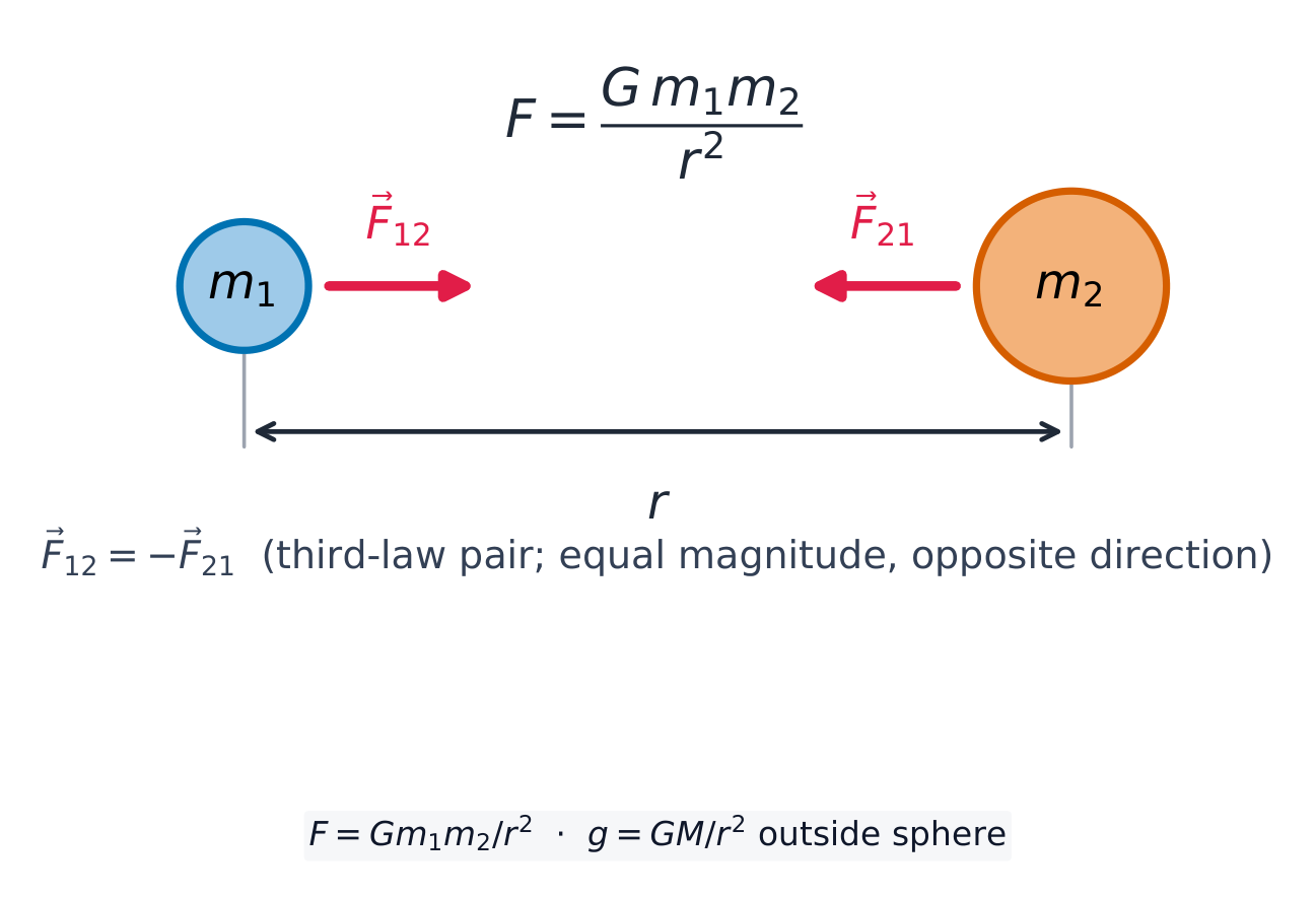
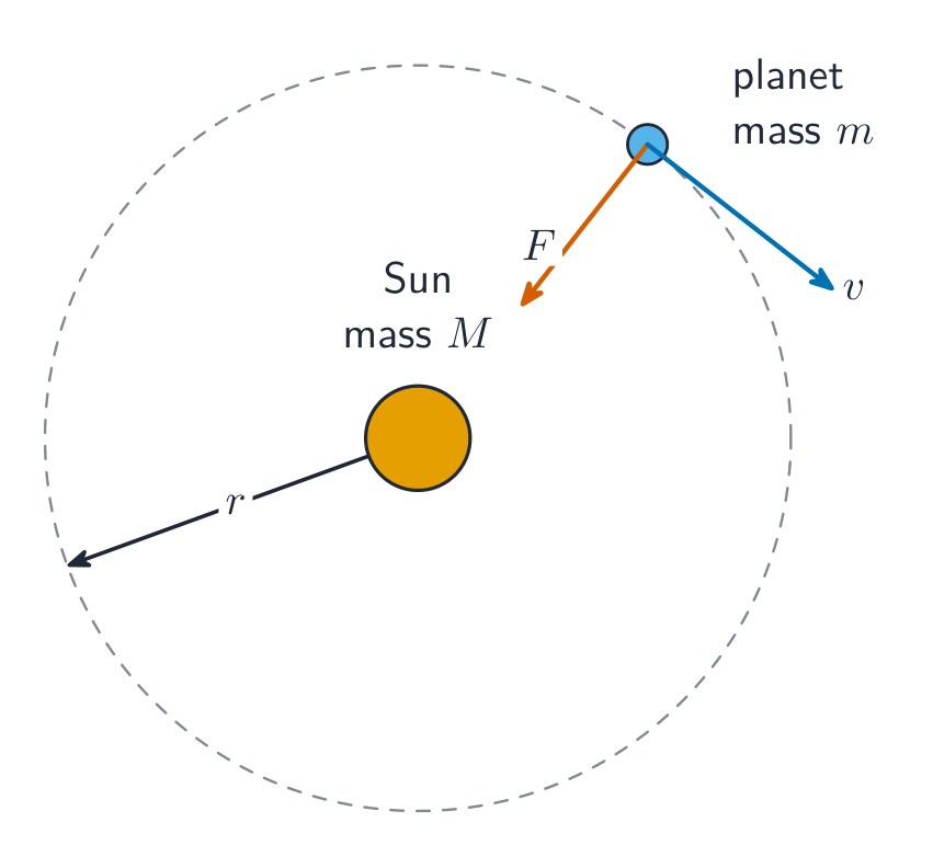
    Dos masas se atraen mutuamente con fuerzas inversamente proporcionales al cuadrado de la distancia, iguales y opuestas, a lo largo de la línea que las une
    Dos masas se atraen mutuamente con fuerzas iguales, opuestas y de inverso cuadrado a lo largo de la línea que las une
    2.7

    Kinetic and Static Friction · ⁨Fricción cinética y estática⁩

    Syllabus
    English

    Learning Objective 2.7.A: Describe kinetic friction between two surfaces.

    • 2.7.A.1 Kinetic friction occurs when two surfaces in contact move relative to each other.
      • 2.7.A.1.i The kinetic friction force is exerted in a direction opposite the motion of each surface relative to the other surface.
      • 2.7.A.1.ii The force of friction between two surfaces does not depend on the size of the surface area of contact.
    • 2.7.A.2 The magnitude of the kinetic friction force exerted on an object is the product of the normal force the surface exerts on the object and the coefficient of kinetic friction.
      • Equation: $\left| \vec{F}_{f,k} \right| = \left| \mu_k \vec{F}_N \right|$
      • 2.7.A.2.i The coefficient of kinetic friction depends on the material properties of the surfaces that are in contact.
      • 2.7.A.2.ii Normal force is the perpendicular component of the force exerted on an object by the surface with which it is in contact; it is directed away from the surface.

    Learning Objective 2.7.B: Describe static friction between two surfaces.

    • 2.7.B.1 Static friction may occur between the contacting surfaces of two objects that are not moving relative to each other.
    • 2.7.B.2 Static friction adopts the value and direction required to prevent an object from slipping or sliding on a surface.
      • Equation: $\left| \vec{F}_{f,s} \right| \leq \left| \mu_s \vec{F}_n \right|$
      • 2.7.B.2.i Slipping and sliding refer to situations in which two surfaces are moving relative to each other.
      • 2.7.B.2.ii There exists a maximum value for which static friction will prevent an object from slipping on a given surface.
        • Derived equation: $F_{f,s,\text{max}} = \mu_s F_N$
    • 2.7.B.3 The coefficient of static friction is typically greater than the coefficient of kinetic friction for a given pair of surfaces.
    Español

    Objetivo de aprendizaje 2.7.A: Describir la fricción cinética entre dos superficies.

    • 2.7.A.1 La fricción cinética ocurre cuando dos superficies en contacto se mueven relativamente una respecto a la otra.
      • 2.7.A.1.i La fuerza de fricción cinética se ejerce en dirección opuesta al movimiento de cada superficie relativa a la otra.
      • 2.7.A.1.ii La fuerza de fricción entre dos superficies no depende del tamaño del área de contacto.
    • 2.7.A.2 La magnitud de la fuerza de fricción cinética ejercida sobre un objeto es el producto de la fuerza normal que la superficie ejerce sobre el objeto y el coeficiente de fricción cinética.
      • Ecuación: $\left| \vec{F}_{f,k} \right| = \left| \mu_k \vec{F}_N \right|$
      • 2.7.A.2.i El coeficiente de fricción cinética depende de las propiedades del material de las superficies que están en contacto.
      • 2.7.A.2.ii La fuerza normal es la componente perpendicular de la fuerza que ejerce una superficie sobre un objeto con el que está en contacto; se dirige alejándose de la superficie.

    Objetivo de aprendizaje 2.7.B: Describir la fricción estática entre dos superficies.

    • 2.7.B.1 La fricción estática puede ocurrir entre las superficies de contacto de dos objetos que no se mueven relativamente una respecto a la otra.
    • 2.7.B.2 La fricción estática adopta el valor y la dirección necesarios para evitar que un objeto resbale o deslice sobre una superficie.
      • Ecuación: $\left| \vec{F}_{f,s} \right| \leq \left| \mu_s \vec{F}_n \right|$
      • 2.7.B.2.i Resbalar y deslizar se refieren a situaciones en las que dos superficies se mueven relativamente una respecto a la otra.
      • 2.7.B.2.ii Existe un valor máximo para el cual la fricción estática evitará que un objeto resbale sobre una superficie dada.
        • Ecuación derivada: $F_{f,s,\text{max}} = \mu_s F_N$
    • 2.7.B.3 El coeficiente de fricción estática suele ser mayor que el coeficiente de fricción cinética para un par dado de superficies.

    Source: College Board AP Course and Exam Description · ⁨Fuente: College Board AP Course and Exam Description⁩

    English

    Friction 摩擦力 opposes sliding along a surface: kinetic 动摩擦 $f_k=\mu_k N$ while sliding, and static 静摩擦 $f_s\le\mu_s N$ up to a maximum before sliding. $N$ is the normal force 法向力. Note the inequality: static friction is only as large as it needs to be, and $\mu_s N$ is its ceiling, not its value.

    Worked example. The same block on the same $30^{\circ}$ incline, now with $\mu_k=0.20$. Perpendicular to the ramp: $N=mg\cos30^{\circ}$. Along the ramp: $ma=mg\sin30^{\circ}-\mu_k mg\cos30^{\circ}$, so $a=g(\sin30^{\circ}-0.20\cos30^{\circ})=9.8(0.500-0.173)=3.2\ \text{m/s}^2$ – the mass cancels again.

    Español

    La fricción 摩擦力 se opone al deslizamiento a lo largo de una superficie: cinética 动摩擦 $f_k=\mu_k N$ mientras se desliza, y estática 静摩擦 $f_s\le\mu_s N$ hasta un máximo antes de deslizarse. $N$ es la fuerza normal 法向力. Nota la desigualdad: la fricción estática es tan grande como necesita ser, y $\mu_s N$ es su techo, no su valor.

    Ejemplo resuelto. El mismo bloque en el mismo plano inclinado de $30^{\circ}$, ahora con $\mu_k=0.20$. Perpendicular al plano: $N=mg\cos30^{\circ}$. A lo largo del plano: $ma=mg\sin30^{\circ}-\mu_k mg\cos30^{\circ}$, así que $a=g(\sin30^{\circ}-0.20\cos30^{\circ})=9.8(0.500-0.173)=3.2\ \text{m/s}^2$ – la masa se cancela nuevamente.

    Explore · ⁨Explorar⁩

    Deslizar un bloque por una pendiente con fricción

    La fricción se opone al movimiento hasta un máximo $\mu N$. Inclina la pendiente hasta que la atracción de la gravedad a lo largo de ella supere la fricción estática y el bloque comience a deslizarse.

    2.8

    Spring Forces · ⁨Fuerzas de resortes⁩

    Syllabus
    English

    Learning Objective 2.8.A: Describe the force exerted on an object by an ideal spring.

    • 2.8.A.1 An ideal spring has negligible mass and exerts a force that is proportional to the change in its length as measured from its relaxed length. A nonideal spring either has nonnegligible mass or exerts a force that is not proportional to the change in its length as measured from its relaxed length.
    • 2.8.A.2 The magnitude of the force exerted by an ideal spring on an object is given by Hooke's law:
      • Equation: $\vec{F}_s = -k \Delta \vec{x}$
    • 2.8.A.3 The force exerted on an object by a spring is always directed toward the equilibrium position of the object–spring system.

    Learning Objective 2.8.B: Describe the equivalent spring constant of a combination of springs exerting forces on an object.

    • 2.8.B.1 A collection of springs that exert forces on an object may behave as though they were a single spring with an equivalent spring constant $k_{\text{eq}}$.
      • 2.8.B.1.i The inverse of the equivalent spring constant of a set of springs in series is equal to the sum of the inverses of the individual spring constants.
        • Derived equation: $\dfrac{1}{k_{\text{eq, series}}} = \sum_i \dfrac{1}{k_i} = \dfrac{1}{k_1} + \dfrac{1}{k_2} + \dots$
      • 2.8.B.1.ii The equivalent spring constant of a set of springs arranged in series is smaller than the smallest constituent spring constant.
      • 2.8.B.1.iii The equivalent spring constant of a set of springs arranged in parallel is the sum of the individual spring constants.
        • Derived equation: $k_{\text{eq, parallel}} = \sum_i k_i = k_1 + k_2 + \dots$

    Boundary statement: AP Physics C: Mechanics only expects students to find the effective spring constant of systems of springs that are arranged either in series or in parallel and does not expect students to find the effective spring constant of a system in which springs are arranged in both series and parallel.

    Español

    Objetivo de Aprendizaje 2.8.A: Describir la fuerza que ejerce un resorte ideal sobre un objeto.

    • 2.8.A.1 Un resorte ideal tiene masa despreciable y ejerce una fuerza proporcional al cambio en su longitud medida desde su longitud relajada. Un resorte no ideal tiene una masa no despreciable o ejerce una fuerza que no es proporcional al cambio en su longitud medida desde su longitud relajada.
    • 2.8.A.2 La magnitud de la fuerza ejercida por un resorte ideal sobre un objeto viene dada por la ley de Hooke:
      • Ecuación: $\vec{F}_s = -k \Delta \vec{x}$
    • 2.8.A.3 La fuerza ejercida sobre un objeto por un resorte siempre está dirigida hacia la posición de equilibrio del sistema objeto-resorte.

    Objetivo de Aprendizaje 2.8.B: Describir la constante elástica equivalente de una combinación de resortes que ejercen fuerzas sobre un objeto.

    • 2.8.B.1 Un conjunto de resortes que ejercen fuerzas sobre un objeto puede comportarse como si fueran un solo resorte con una constante elástica equivalente $k_{\text{eq}}$.
      • 2.8.B.1.i El inverso de la constante elástica equivalente de un conjunto de resortes en serie es igual a la suma de los inversos de las constantes elásticas individuales.
        • Ecuación derivada: $\dfrac{1}{k_{\text{eq, series}}} = \sum_i \dfrac{1}{k_i} = \dfrac{1}{k_1} + \dfrac{1}{k_2} + \dots$
      • 2.8.B.1.ii La constante elástica equivalente de un conjunto de resortes dispuestos en serie es menor que la constante elástica más pequeña de sus componentes.
      • 2.8.B.1.iii La constante elástica equivalente de un conjunto de resortes dispuestos en paralelo es la suma de las constantes elásticas individuales.
        • Ecuación derivada: $k_{\text{eq, parallel}} = \sum_i k_i = k_1 + k_2 + \dots$

    Declaración de límites: AP Physics C: Mechanics solo espera que los estudiantes encuentren la constante elástica efectiva de sistemas de resortes dispuestos ya sea en serie o en paralelo, y no espera que los estudiantes encuentren la constante elástica efectiva de un sistema en el que los resortes están dispuestos tanto en serie como en paralelo.

    Source: College Board AP Course and Exam Description · ⁨Fuente: College Board AP Course and Exam Description⁩

    English
    Hooke's law & the elastic limit

    An ideal spring obeys Hooke's law 胡克定律 $F_s=-kx$, a restoring force set by the spring constant 弹簧劲度系数 $k$. Its stored energy is $U=\tfrac12 kx^2$.

    Combined springs act as one equivalent spring of constant $k_{\text{eq}}$. In parallel (side by side, sharing the load) the constants add, $k_{\text{eq}}=k_1+k_2$ – stiffer than either. In series (end to end) they combine as $\dfrac{1}{k_{\text{eq}}}=\dfrac{1}{k_1}+\dfrac{1}{k_2}$ – softer than the softest one. Two springs pulling a mass from opposite sides also act in parallel, giving a restoring constant $k_1+k_2$. Whichever you have, the SHM period uses $k_{\text{eq}}$: $T=2\pi\sqrt{m/k_{\text{eq}}}$.

    Español
    La ley de Hooke y el límite elástico

    Un resorte ideal obedece la Ley de Hooke 胡克定律 $F_s=-kx$, una fuerza restauradora determinada por la constante del resorte 弹簧劲度系数 $k$. Su energía almacenada es $U=\tfrac12 kx^2$.

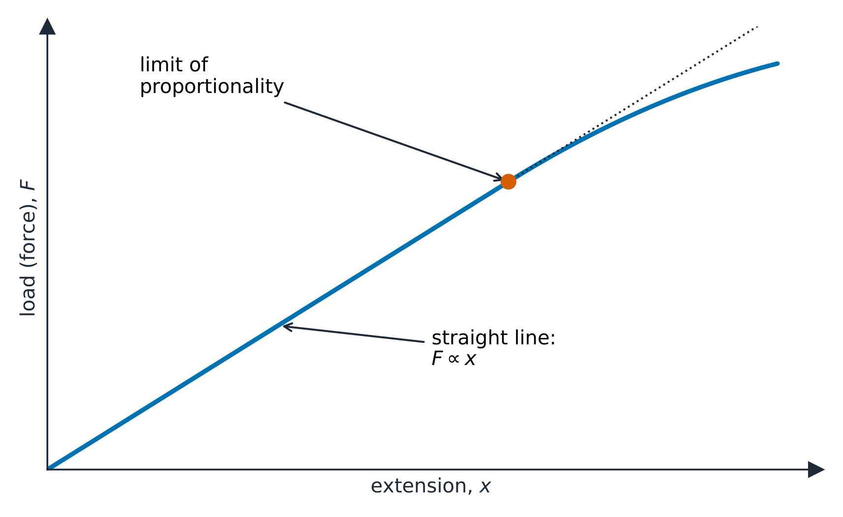
    La ley de Hooke: la extensión es proporcional a la carga hasta el límite de proporcionalidad
    Ley de Hooke: la extensión es proporcional a la carga hasta el límite de proporcionalidad

    Los resortes combinados actúan como un único resorte equivalente de constante $k_{\text{eq}}$. En paralelo (uno al lado del otro, compartiendo la carga) las constantes se suman, $k_{\text{eq}}=k_1+k_2$ – más rígido que cualquiera de ellos. En serie (extremo con extremo) se combinan como $\dfrac{1}{k_{\text{eq}}}=\dfrac{1}{k_1}+\dfrac{1}{k_2}$ – más blando que el más blando. Dos resortes jalando una masa desde lados opuestos también actúan en paralelo, dando una constante restauradora $k_1+k_2$. Sea cual sea tu configuración, el periodo de MSJ usa $k_{\text{eq}}$: $T=2\pi\sqrt{m/k_{\text{eq}}}$.
    Explore · ⁨Explorar⁩

    Estirar un resorte (Ley de Hooke)

    La fuerza de un resorte es proporcional a su extensión, $F=kx$ (Ley de Hooke). Tira con más fuerza y la extensión crece al mismo ritmo — hasta el límite del resorte.

    Vocabulary · ⁨Vocabulario⁩ Train · ⁨Entrenar⁩
    English · ⁨Inglés⁩ Chinese · ⁨Chino⁩ Pinyin
    Hooke's law/hʊks lɔː/ 胡克定律 hú kè dìng lǜ
    spring constant/sprɪŋ ˈkɒnstənt/ 弹簧劲度系数 tán huáng jìn dù xì shù
    resistive force/rɪˈzɪstɪv fɔːs/ 阻力 zǔ lì
    2.9

    Resistive Forces · ⁨Fuerzas Resistivas⁩

    Syllabus
    English

    Learning Objective 2.9.A: Describe the motion of an object subject to a resistive force.

    • 2.9.A.1 A resistive force is defined as a velocity-dependent force in the opposite direction of an object's velocity, for example:
      • Equation: $\vec{F}_r = -k\vec{v}$
    • 2.9.A.2 Applying Newton's second law to an object upon which a resistive force is exerted results in a differential equation for velocity.
      • 2.9.A.2.i Using the method of separation of variables, the velocity can be determined by integrating over the proper limits of integration.
      • 2.9.A.2.ii The acceleration or position of a moving object that is subject to a velocity-dependent force may be determined using initial conditions of the object and methods of calculus, once a function for velocity is determined.
      • 2.9.A.2.iii The position, velocity, and acceleration as functions of time of an object under the influence of a resistive force of the form $\vec{F}_r = -k\vec{v}$ are exponential and have asymptotes that are determined by the initial conditions of the object and the forces exerted on the object.
    • 2.9.A.3 Terminal velocity is defined as the maximum speed achieved by an object moving under the influence of a constant force and a resistive force that are exerted on the object in opposite directions. The terminal condition is reached when the net force exerted on the object is zero.
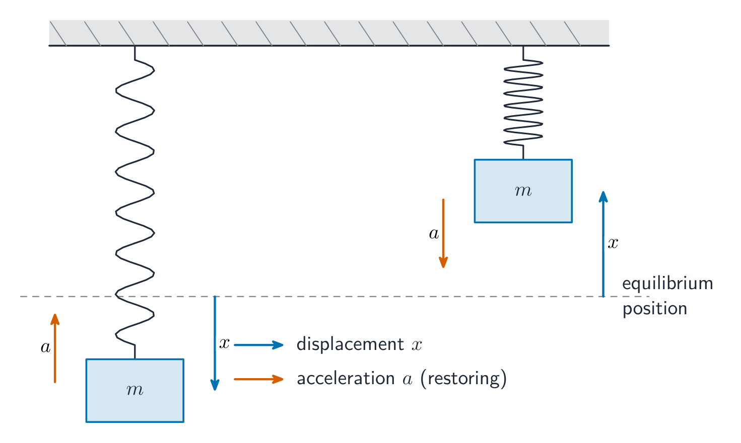
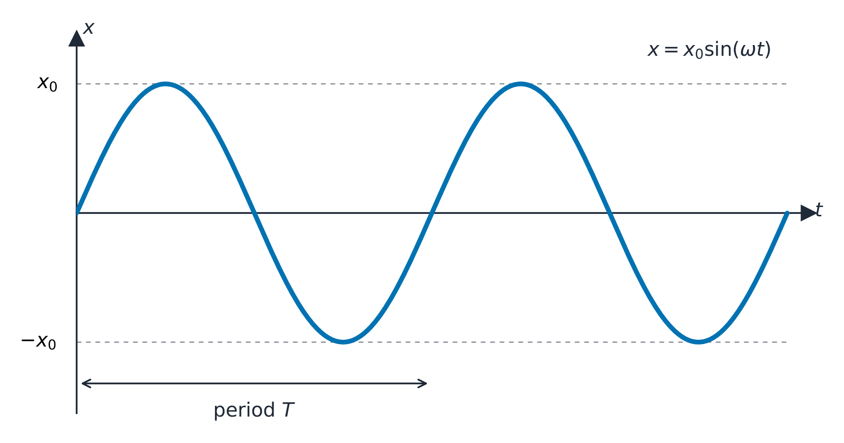
    Español

    Objetivo de Aprendizaje 2.9.A: Describir el movimiento de un objeto sujeto a una fuerza de resistencia.

    • 2.9.A.1 Una fuerza de resistencia se define como una fuerza dependiente de la velocidad en dirección opuesta a la velocidad del objeto, por ejemplo:
      • Ecuación: $\vec{F}_r = -k\vec{v}$
    • 2.9.A.2 La aplicación de la segunda ley de Newton a un objeto sobre el cual actúa una fuerza de resistencia da lugar a una ecuación diferencial para la velocidad.
      • 2.9.A.2.i Utilizando el método de separación de variables, la velocidad puede determinarse integrando sobre los límites de integración adecuados.
      • 2.9.A.2.ii La aceleración o posición de un objeto en movimiento que está sujeto a una fuerza dependiente de la velocidad pueden determinarse mediante condiciones iniciales del objeto y métodos del cálculo, una vez obtenida una función para la velocidad.
      • 2.9.A.2.iii La posición, la velocidad y la aceleración como funciones del tiempo de un objeto bajo la influencia de una fuerza de resistencia de la forma $\vec{F}_r = -k\vec{v}$ son exponenciales y tienen asíntotas determinadas por las condiciones iniciales del objeto y las fuerzas que actúan sobre él.
    • 2.9.A.3 La velocidad terminal se define como la velocidad máxima alcanzada por un objeto que se mueve bajo la influencia de una fuerza constante y una fuerza de resistencia que actúan sobre el objeto en direcciones opuestas. Se alcanza la condición terminal cuando la fuerza neta ejercida sobre el objeto es cero.

    Source: College Board AP Course and Exam Description · ⁨Fuente: College Board AP Course and Exam Description⁩

    English

    A resistive force 阻力 (drag) opposes motion through a fluid and grows with speed, often modeled as $F=-bv$ or $F=-cv^2$. Newton's second law then gives a differential equation, e.g. $m\dfrac{dv}{dt}=mg-bv$ for a falling object. As speed rises, drag builds until it balances the driving force; the object then stops accelerating and moves at a constant terminal velocity 终极速度, found by setting the net force (and $dv/dt$) to zero.

    Worked example. For a falling object with $m\dfrac{dv}{dt}=mg-bv$, the terminal velocity is where $\dfrac{dv}{dt}=0$: $mg=bv_T$, so $v_T=\dfrac{mg}{b}$. With $m=0.10\ \text{kg}$ and $b=0.50\ \text{kg/s}$, $v_T=\dfrac{0.10(9.8)}{0.50}=2.0\ \text{m/s}$.

    To get the full motion $v(t)$, separate the variables 分离变量 and integrate from rest:

    $$\int_0^{v}\frac{dv'}{mg-bv'}=\int_0^{t}\frac{dt'}{m}\;\Rightarrow\;-\frac{1}{b}\ln\!\frac{mg-bv}{mg}=\frac{t}{m},$$
    which rearranges to $v(t)=v_T\left(1-e^{-bt/m}\right)$ – the speed rising exponentially toward $v_T$. Showing this integration is the calculus skill a Physics C free-response rewards, not just quoting the final formula.

    Español

    Una fuerza resistente 阻力 (arrastre/drag) se opone al movimiento a través de un fluido y crece con la velocidad, modelada a menudo como $F=-bv$ o $F=-cv^2$. La segunda ley de Newton da entonces una ecuación diferencial, ej. $m\dfrac{dv}{dt}=mg-bv$ para un objeto cayendo. A medida que aumenta la velocidad, el arrastre crece hasta equilibrar la fuerza motriz; el objeto deja de acelerar y se mueve a una velocidad terminal 终极 velocidad constante, encontrada igualando a cero la fuerza neta (y $dv/dt$).

    Ejemplo resuelto. Para un objeto cayendo con $m\dfrac{dv}{dt}=mg-bv$, la velocidad terminal es donde $\dfrac{dv}{dt}=0$: $mg=bv_T$, así que $v_T=\dfrac{mg}{b}$. Con $m=0.10\ \text{kg}$ y $b=0.50\ \text{kg/s}$, $v_T=\dfrac{0.10(9.8)}{0.50}=2.0\ \text{m/s}$.

    Para obtener el movimiento completo $v(t)$, separar variables 分离变量 e integrar desde el reposo:

    $$\int_0^{v}\frac{dv'}{mg-bv'}=\int_0^{t}\frac{dt'}{m}\;\Rightarrow\;-\frac{1}{b}\ln\!\frac{mg-bv}{mg}=\frac{t}{m},$$
    que se reorganiza en $v(t)=v_T\left(1-e^{-bt/m}\right)$ – la velocidad sube exponencialmente hacia $v_T$. Mostrar esta integración es la habilidad de cálculo que recompensa la respuesta libre de Física C, no solo citar la fórmula final.

    Un objeto que cae a través de un fluido acelera hasta alcanzar una velocidad terminal
    Un objeto cayendo a través de un fluido acelera hasta alcanzar una velocidad terminal
    Paracaidistas en caída libre: la resistencia aumenta con la velocidad hasta equilibrar el peso en la velocidad terminal
    Paracaidistas en caída libre: el arrastre crece con la velocidad hasta equilibrar el peso en la velocidad terminal
    Vocabulary · ⁨Vocabulario⁩ Train · ⁨Entrenar⁩
    English · ⁨Inglés⁩ Chinese · ⁨Chino⁩ Pinyin
    terminal velocity/ˈtɜːmɪnl vəˈlɒsɪti/ 终极速度 zhōng jí sù dù
    separate the variables/ˈseprət ðə ˈveərɪəblz/ 分离变量 fēn lí biàn liàng
    centripetal acceleration/senˈtrɪpɪtl əkˌseləˈreɪʃn/ 向心加速度 xiàng xīn jiā sù dù
    2.10

    Circular Motion · ⁨Movimiento circular⁩

    Syllabus
    English

    Learning Objective 2.10.A: Describe the motion of an object traveling in a circular path.

    • 2.10.A.1 Centripetal acceleration is the component of an object's acceleration directed toward the center of the object's circular path.
      • 2.10.A.1.i The magnitude of centripetal acceleration for an object moving in a circular path is the ratio of the object's tangential speed squared to the radius of the circular path.
        • Equation: $a_c = \dfrac{v^2}{r}$
      • 2.10.A.1.ii Centripetal acceleration is directed toward the center of an object's circular path.
    • 2.10.A.2 Centripetal acceleration can result from a single force, more than one force, or components of forces that are exerted on an object in circular motion.
      • 2.10.A.2.i At the top of a vertical, circular loop, an object requires a minimum speed to maintain circular motion. At this point, and with this minimum velocity, the gravitational force is the only force that causes the centripetal acceleration.
        • Derived equation: $v = \sqrt{gr}$
      • 2.10.A.2.ii Components of the static friction force and the normal force can contribute to the net force producing centripetal acceleration of an object traveling in a circle on a banked surface.
      • 2.10.A.2.iii A component of tension contributes to the net force producing centripetal acceleration experienced by a conical pendulum.
    • 2.10.A.3 Tangential acceleration is the rate at which an object's speed changes and is directed tangent to the object's circular path.
    • 2.10.A.4 The net acceleration of an object moving in a circle is the vector sum of the centripetal acceleration and tangential acceleration.
    • 2.10.A.5 The revolution of an object traveling in a circular path at a constant speed (uniform circular motion) can be described using period and frequency.
      • 2.10.A.5.i The time to complete one full circular path, one full rotation, or a full cycle of oscillatory motion is defined as period, $T$.
      • 2.10.A.5.ii The rate at which an object is completing revolutions is defined as frequency, $f$.
        • Equation: $T = \dfrac{1}{f}$
      • 2.10.A.5.iii For an object traveling at a constant speed in a circular path, the period is given by the derived equation
        • Derived equation: $T = \dfrac{2\pi r}{v}$

    Learning Objective 2.10.B: Describe circular orbits using Kepler's third law.

    • 2.10.B.1 For a satellite in circular orbit around a central body, the satellite's centripetal acceleration is caused only by gravitational attraction. The period and radius of the circular orbit are related to the mass of the central body.
      • Derived equation: $T^2 = \dfrac{4\pi^2}{GM} R^3$

    Boundary statement: AP Physics C: Mechanics does not expect students to know Kepler's first or second laws of planetary motion.

    Español

    Objetivo de aprendizaje 2.10.A: Describir el movimiento de un objeto que se desplaza en una trayectoria circular.

    • 2.10.A.1 La aceleración centrípeta es la componente de la aceleración de un objeto dirigida hacia el centro de su trayectoria circular.
      • 2.10.A.1.i La magnitud de la aceleración centrípeta para un objeto que se mueve en una trayectoria circular es la razón entre el cuadrado de la velocidad tangencial del objeto y el radio de la trayectoria circular.
        • Ecuación: $a_c = \dfrac{v^2}{r}$
      • 2.10.A.1.ii La aceleración centrípeta está dirigida hacia el centro de la trayectoria circular del objeto.
    • 2.10.A.2 La aceleración centrípeta puede ser producida por una sola fuerza, por más de una fuerza o por componentes de fuerzas que actúan sobre un objeto en movimiento circular.
      • 2.10.A.2.i En la parte superior de un bucle vertical circular, un objeto requiere una velocidad mínima para mantener el movimiento circular. En este punto y con esta velocidad mínima, la fuerza gravitacional es la única fuerza que produce la aceleración centrípeta.
        • Ecuación derivada: $v = \sqrt{gr}$
      • 2.10.A.2.ii Las componentes de la fuerza de fricción estática y la fuerza normal pueden contribuir a la fuerza neta que produce la aceleración centrípeta de un objeto que se desplaza en un círculo sobre una superficie inclinada (bancada).
      • 2.10.A.2.iii Una componente de la tensión contribuye a la fuerza neta que produce la aceleración centrípeta experimentada por un péndulo cónico.
    • 2.10.A.3 La aceleración tangencial es la tasa a la cual cambia la rapidez de un objeto y está dirigida tangente a la trayectoria circular del objeto.
    • 2.10.A.4 La aceleración neta de un objeto que se mueve en un círculo es la suma vectorial de la aceleración centrípeta y la aceleración tangencial.
    • 2.10.A.5 La revolución de un objeto que se desplaza en una trayectoria circular a velocidad constante (movimiento circular uniforme) puede describirse utilizando el periodo y la frecuencia.
      • 2.10.A.5.i El tiempo necesario para completar una trayectoria circular completa, una rotación completa o un ciclo completo de movimiento oscilatorio se define como periodo, $T$.
      • 2.10.A.5.ii La tasa a la que un objeto completa revoluciones se define como frecuencia, $f$.
        • Ecuación: $T = \dfrac{1}{f}$
      • 2.10.A.5.iii Para un objeto que se desplaza a velocidad constante en una trayectoria circular, el periodo viene dado por la ecuación derivada:
        • Ecuación derivada: $T = \dfrac{2\pi r}{v}$

    Objetivo de aprendizaje 2.10.B: Describir órbitas circulares usando la tercera ley de Kepler.

    • 2.10.B.1 Para un satélite en órbita circular alrededor de un cuerpo central, la aceleración centrípeta del satélite es causada únicamente por la atracción gravitacional. El periodo y el radio de la órbita circular están relacionados con la masa del cuerpo central.
      • Ecuación derivada: $T^2 = \dfrac{4\pi^2}{GM} R^3$

    Enunciado de límite: AP Physics C: Mechanics no espera que los estudiantes conozcan la primera ni la segunda ley del movimiento planetario de Kepler.

    Source: College Board AP Course and Exam Description · ⁨Fuente: College Board AP Course and Exam Description⁩

    English
    Uniform circular motion

    Uniform circular motion has a centripetal acceleration 向心加速度 $a_c=\dfrac{v^2}{r}$ pointing to the center, requiring a net inward force $F_c=\dfrac{mv^2}{r}$ supplied by a real force (tension, gravity, friction, normal). There is no outward force. For vertical circles and banked curves, decompose the real forces to find which provides the centripetal requirement.

    Worked example. A $0.50\ \text{kg}$ ball is whirled on a $1.0\ \text{m}$ string in a horizontal circle at $3.0\ \text{m/s}$. The string tension supplies the whole centripetal force: $T=\dfrac{mv^2}{r}=\dfrac{0.50(3.0)^2}{1.0}=4.5\ \text{N}$.

    Worked example (vertical circle). At the top of a vertical loop of radius $r$, gravity and the normal force both point toward the center: $N+mg=\dfrac{mv^2}{r}$. The slowest possible speed at the top is where the track pushes with nothing at all ($N=0$): $v_{\min}=\sqrt{gr}$. For $r=2.5\ \text{m}$: $v_{\min}=\sqrt{9.8(2.5)}=4.9\ \text{m/s}$. Any slower and the cart leaves the track before the top.

    Español
    Movimiento circular uniforme

    El movimiento circular uniforme tiene una aceleración centrípeta 向心加速度 $a_c=\dfrac{v^2}{r}$ apuntando hacia el centro, requiriendo una fuerza neta hacia adentro $F_c=\dfrac{mv^2}{r}$ suministrada por una fuerza real (tensión, gravedad, fricción, normal). No hay fuerza hacia afuera. Para círculos verticales y curvas peraltadas, descompón las fuerzas reales para encontrar cuál satisface el requisito centrípeto.

    Ejemplo resuelto. Una bola de $0.50\ \text{kg}$ se gira en una cuerda de $1.0\ \text{m}$ en un círculo horizontal a $3.0\ \text{m/s}$. La tensión de la cuerda suministra toda la fuerza centrípeta: $T=\dfrac{mv^2}{r}=\dfrac{0.50(3.0)^2}{1.0}=4.5\ \text{N}$.

    Ejemplo resuelto (círculo vertical). En la parte superior de un bucle vertical de radio $r$, tanto la gravedad como la fuerza normal apuntan hacia el centro: $N+mg=\dfrac{mv^2}{r}$. La velocidad más lenta posible en la parte superior es donde la pista ya no empuja ($N=0$): $v_{\min}=\sqrt{gr}$. Para $r=2.5\ \text{m}$: $v_{\min}=\sqrt{9.8(2.5)}=4.9\ \text{m/s}$. Si va más lento, el carrito saldrá de la pista antes de llegar a la cima.

    La velocidad apunta a lo largo de la tangente; la fuerza centrípeta apunta hacia el centro
    La velocidad apunta a lo largo de la tangente; la fuerza centrípeta apunta hacia el centro
    2.10

    Exam tips · ⁨Consejos para el examen⁩

    English
    • Locate the center of mass with $x_{cm}=\tfrac{1}{M}\int x\,dm$ (or $\tfrac{\sum m_i x_i}{\sum m_i}$ for point masses) and use $\lambda,\sigma,\rho$ for the mass element.
    • The net external force moves the center of mass as if all mass sat there: $\vec F_{net}=M\vec a_{cm}$.
    • Define your system clearly — internal forces cancel, so only external forces change its momentum.
    • Exploit symmetry to shortcut a center-of-mass integral.
    • Distinguish center of mass from center of gravity (identical in a uniform field).
    Español
    • Ubica el centro de masa con $x_{cm}=\tfrac{1}{M}\int x\,dm$ (o $\tfrac{\sum m_i x_i}{\sum m_i}$ para masas puntuales) y usa $\lambda,\sigma,\rho$ para el elemento de masa.
    • La fuerza externa neta mueve el centro de masa como si toda la masa estuviera allí: $\vec F_{net}=M\vec a_{cm}$.
    • Define claramente tu sistema – las fuerzas internas se cancelan, así que solo las fuerzas externas cambian su momento.
    • Explota la simetría para simplificar una integral del centro de masa.
    • Distingue entre centro de masa y centro de gravedad (idénticos en un campo uniforme).
  • 3

    Trabajo, energía y potencia

    Watch lesson · ⁨Ver lección⁩
    3.1

    Translational Kinetic Energy · ⁨Energía Cinética de Traslación⁩

    Syllabus
    English

    Learning Objective 3.1.A: Describe the translational kinetic energy of an object in terms of the object's mass and velocity.

    • 3.1.A.1 An object's translational kinetic energy is given by the equation
      • Equation: $K = \dfrac{1}{2}mv^2$
    • 3.1.A.2 Translational kinetic energy is a scalar quantity.
    • 3.1.A.3 Different observers may measure different values of the translational kinetic energy of an object, depending on the observer's frame of reference.
    Español

    Objetivo de Aprendizaje 3.1.A: Describir la energía cinética traslacional de un objeto en términos de la masa y la velocidad del mismo.

    • 3.1.A.1 La energía cinética traslacional de un objeto viene dada por la ecuación
      • Ecuación: $K = \dfrac{1}{2}mv^2$
    • 3.1.A.2 La energía cinética traslacional es una cantidad escalar.
    • 3.1.A.3 Diferentes observadores pueden medir diferentes valores de la energía cinética traslacional de un objeto, dependiendo del sistema de referencia del observador.

    Source: College Board AP Course and Exam Description · ⁨Fuente: College Board AP Course and Exam Description⁩

    English

    Kinetic energy 动能 is the energy of motion, a scalar 标量 measured in joules 焦耳 (J):

    $$K=\tfrac{1}{2}mv^2.$$

    It grows with the square of speed – doubling the speed quadruples $K$. One subtlety worth knowing: kinetic energy depends on the observer's reference frame 参考系. A passenger walking down a train has a small $K$ measured inside the train and a huge one measured from the ground – both observers are right, each in their own frame.

    Español

    La energía cinética 动能 es la energía del movimiento, una magnitud escalar 标量 medida en jules 焦耳 (J):

    $$K=\tfrac{1}{2}mv^2.$$

    Aumenta con el cuadrado de la velocidad: duplicar la velocidad cuadruplica $K$. Un matiz importante a conocer: la energía cinética depende del sistema de referencia 参考系 del observador. Un pasajero caminando por un tren tiene una pequeña $K$ medida desde dentro del tren y una enorme medida desde el suelo; ambos observadores tienen razón, cada uno en su propio marco de referencia.

    Vocabulary · ⁨Vocabulario⁩ Train · ⁨Entrenar⁩
    English · ⁨Inglés⁩ Chinese · ⁨Chino⁩ Pinyin
    Kinetic energy/kɪˈnetɪk ˈenədʒi/ 动能 dòng néng
    scalar/ˈskeɪlə/ 标量 biāo liàng
    joules/dʒuːlz/ 焦耳 jiāo ěr
    reference frame/ˈrefrəns freɪm/ 参考系 cān kǎo xì
    3.2

    Work · ⁨Trabajo⁩

    Syllabus
    English

    Learning Objective 3.2.A: Describe the work done on an object or system by a given force or collection of forces.

    • 3.2.A.1 Work is the amount of energy transferred into or out of a system by a force exerted on that system over a distance.
      • 3.2.A.1.i The work done by a conservative force exerted on a system is path-independent and only depends on the initial and final configurations of that system.
      • 3.2.A.1.ii The work done by a conservative force on a system—or the change in the potential energy of the system—will be zero if the system returns to its initial configuration.
      • 3.2.A.1.iii Potential energies are associated only with conservative forces.
      • 3.2.A.1.iv The work done by a nonconservative force is path-dependent.
      • 3.2.A.1.v The most common nonconservative forces are friction and air resistance.
    • 3.2.A.2 Work is a scalar quantity that may be positive, negative, or zero.
    • 3.2.A.3 The work done on an object by a variable force is calculated using
      • Equation: $W = \displaystyle\int_a^b \vec{F}(r) \cdot d\vec{r}$, where the integral is taken over the path from point $a$ to point $b$.
      • 3.2.A.3.i The dot product between two vectors, $\vec{A}$ and $\vec{B}$, results in a scalar quantity of magnitude $\vec{A} \cdot \vec{B} = AB\cos\theta$.
      • 3.2.A.3.ii Only the component of the force exerted on a system that is parallel to the displacement of the point of application of the force will change the system's total energy.
      • 3.2.A.3.iii If the component of the force exerted on a system that is parallel to the displacement is constant, the work done on the system by the force is given by the derived equation $W = F_{\parallel}d = Fd\cos\theta$.
      • 3.2.A.3.iv The component of the force exerted on a system perpendicular to the direction of the displacement of the system's center of mass can change the direction of the system's motion without changing the system's kinetic energy.
    • 3.2.A.4 The work–energy theorem states that the change in an object's kinetic energy is equal to the sum of the work (net work) being done by all forces exerted on the object.
      • Equation: $\Delta K = \displaystyle\sum W_i = \sum F_{\parallel,i}\, d_i$
      • 3.2.A.4.i An external force may change the configuration of a system. The component of the external force parallel to the displacement times the displacement of the point of application of the force gives the change in kinetic energy of the system.
      • 3.2.A.4.ii If the system's center of mass and the point of application of the force move the same distance when a force is exerted on a system, then the system may be modeled as an object, and only the system's kinetic energy can change.
      • 3.2.A.4.iii The energy dissipated by friction is typically equated to the force of friction times the length of the path over which the force is exerted.
        • Equation: $\Delta E_{\text{mech}} = F_f d\cos\theta$
      • 3.2.A.5 Work is equal to the area under the curve of a graph of $F_{\parallel}$ as a function of displacement.

    Boundary statement: AP Physics C: Mechanics only expects students to analyze the transfer of mechanical energy, although students should be aware that mechanical energy may be dissipated in the form of thermal energy or sound.

    Español

    Objetivo de aprendizaje 3.2.A: Describir el trabajo realizado sobre un objeto o sistema por una fuerza dada o por un conjunto de fuerzas.

    • 3.2.A.1 El trabajo es la cantidad de energía transferida hacia adentro o hacia afuera de un sistema mediante una fuerza ejercida sobre ese sistema a lo largo de una distancia.
      • 3.2.A.1.i El trabajo realizado por una fuerza conservativa ejercida sobre un sistema es independiente de la trayectoria y depende únicamente de las configuraciones inicial y final del sistema.
      • 3.2.A.1.ii El trabajo realizado por una fuerza conservativa sobre un sistema —o el cambio en la energía potencial del sistema— será cero si el sistema regresa a su configuración inicial.
      • 3.2.A.1.iii Las energías potenciales están asociadas únicamente con fuerzas conservativas.
      • 3.2.A.1.iv El trabajo realizado por una fuerza no conservativa depende de la trayectoria.
      • 3.2.A.1.v Las fuerzas no conservativas más comunes son la fricción y la resistencia del aire.
    • 3.2.A.2 El trabajo es una magnitud escalar que puede ser positiva, negativa o cero.
    • 3.2.A.3 El trabajo realizado sobre un objeto por una fuerza variable se calcula mediante
      • Ecuación: $W = \displaystyle\int_a^b \vec{F}(r) \cdot d\vec{r}$, donde la integral se toma a lo largo de la trayectoria desde el punto $a$ hasta el punto $b$.
      • 3.2.A.3.i El producto punto entre dos vectores, $\vec{A}$ y $\vec{B}$, resulta en una magnitud escalar dada por $\vec{A} \cdot \vec{B} = AB\cos\theta$.
      • 3.2.A.3.ii Solo el componente de la fuerza ejercida sobre un sistema que es paralelo al desplazamiento del punto de aplicación de la fuerza cambiará la energía total del sistema.
      • 3.2.A.3.iii Si el componente de la fuerza ejercida sobre un sistema que es paralelo al desplazamiento es constante, el trabajo realizado sobre el sistema por la fuerza está dado por la ecuación derivada $W = F_{\parallel}d = Fd\cos\theta$.
      • 3.2.A.3.iv El componente de la fuerza ejercida sobre un sistema perpendicular a la dirección del desplazamiento del centro de masa del sistema puede cambiar la dirección del movimiento del sistema sin alterar su energía cinética.
    • 3.2.A.4 El teorema del trabajo y la energía establece que el cambio en la energía cinética de un objeto es igual a la suma del trabajo (trabajo neto) realizado por todas las fuerzas exertidas sobre el objeto.
      • Ecuación: $\Delta K = \displaystyle\sum W_i = \sum F_{\parallel,i}\, d_i$
      • 3.2.A.4.i Una fuerza externa puede cambiar la configuración de un sistema. El componente de la fuerza externa paralelo al desplazamiento multiplicado por el desplazamiento del punto de aplicación de la fuerza da como resultado el cambio en la energía cinética del sistema.
      • 3.2.A.4.ii Si el centro de masa del sistema y el punto de aplicación de la fuerza se desplazan la misma distancia cuando se ejerce una fuerza sobre un sistema, entonces el sistema puede modelarse como un objeto, y solo la energía cinética del sistema puede cambiar.
      • 3.2.A.4.iii La energía disipada por la fricción suele equipararse a la fuerza de fricción multiplicada por la longitud de la trayectoria sobre la cual se ejerce la fuerza.
        • Ecuación: $\Delta E_{\text{mech}} = F_f d\cos\theta$
      • 3.2.A.5 El trabajo es igual al área bajo la curva de un gráfico de $F_{\parallel}$ en función del desplazamiento.

    Enunciado de límite: AP Physics C: Mechanics solo espera que los estudiantes analicen la transferencia de energía mecánica, aunque deben estar conscientes de que la energía mecánica puede disiparse en forma de energía térmica o sonido.

    Source: College Board AP Course and Exam Description · ⁨Fuente: College Board AP Course and Exam Description⁩

    English

    Work 功 is energy transferred into or out of a system by a force acting over a distance. For a variable force it is an integral 积分 along the path:

    $$W=\int_a^b \vec{F}\cdot d\vec{r}=\int F\cos\theta\,dr.$$

    For a constant force this reduces to $W=Fd\cos\theta$; on a force–position graph, work is the area under the curve. Work is a scalar with a sign, and the sign is physics, not bookkeeping:

    • Positive – force has a component along the motion (it speeds the object up).
    • Negative – force opposes the motion (friction 摩擦力 and air drag do negative work).
    • Zero – force perpendicular to the motion (the normal force 法向力 on a sliding block, gravity on a horizontal move, tension in a circular swing).

    The work–energy theorem 动能定理 collects every force's contribution: the net work equals the change in kinetic energy,

    $$W_{\text{net}}=\sum W_i=\Delta K.$$

    Worked example. A variable force $F(x)=3x^2\ \text{N}$ (along the motion) acts from $x=0$ to $x=2\ \text{m}$: $W=\displaystyle\int_0^2 3x^2\,dx=\big[x^3\big]_0^2=8\ \text{J}$. Acting alone on a body starting from rest, it would raise the kinetic energy to exactly $8\ \text{J}$.

    Español

    El trabajo 功 es la energía transferida hacia o fuera de un sistema mediante una fuerza que actúa sobre una distancia. Para una fuerza variable, es una integral 积分 a lo largo de la trayectoria:

    $$W=\int_a^b \vec{F}\cdot d\vec{r}=\int F\cos\theta\,dr.$$

    Para una fuerza constante, esto se reduce a $W=Fd\cos\theta$; en una gráfica de fuerza contra posición, el trabajo es el área bajo la curva. El trabajo es un escalar con signo, y ese signo es física, no contabilidad:

    • Positivo – la fuerza tiene una componente a lo largo del movimiento (acelera al objeto).
    • Negativo – la fuerza se opone al movimiento (fricción 摩擦力 y la resistencia del aire realizan trabajo negativo).
    • Cero – la fuerza es perpendicular al movimiento (la fuerza normal 法向力 sobre un bloque deslizante, la gravedad en un movimiento horizontal, la tensión en un balanceo circular).
    Solo la componente de la fuerza a lo largo del desplazamiento realiza trabajo
    Solo la componente de la fuerza a lo largo del desplazamiento realiza trabajo

    El teorema del trabajo y la energía 动能定理 recopila la contribución de todas las fuerzas: el trabajo neto es igual al cambio en la energía cinética,

    $$W_{\text{net}}=\sum W_i=\Delta K.$$

    Ejemplo resuelto. Una fuerza variable $F(x)=3x^2\ \text{N}$ (a lo largo del movimiento) actúa desde $x=0$ hasta $x=2\ \text{m}$: $W=\displaystyle\int_0^2 3x^2\,dx=\big[x^3\big]_0^2=8\ \text{J}$. Actuando sola sobre un cuerpo que parte del reposo, elevaría la energía cinética exactamente a $8\ \text{J}$.

    Vocabulary · ⁨Vocabulario⁩ Train · ⁨Entrenar⁩
    English · ⁨Inglés⁩ Chinese · ⁨Chino⁩ Pinyin
    Work/wɜːk/ 功 gōng
    integral/ˈɪntɪɡrəl/ 积分 jī fēn
    friction/ˈfrɪkʃn/ 摩擦力 mó cā lì
    normal force/ˈnɔːml fɔːs/ 法向力 fǎ xiàng lì
    work–energy theorem/wɜːk ˈenədʒi ˈθɪərəm/ 动能定理 dòng néng dìng lǐ
    3.3

    Potential Energy · ⁨Energía Potencial⁩

    Syllabus
    English

    Learning Objective 3.3.A: Describe the potential energy of a system.

    • 3.3.A.1 A system composed of two or more objects has potential energy if the objects within that system only interact with each other through conservative forces.
    • 3.3.A.2 Potential energy is a scalar quantity associated with the position of objects within a system.
    • 3.3.A.3 The definition of zero potential energy for a given system is a decision made by the observer considering the situation to simplify or otherwise assist in analysis.
    • 3.3.A.4 The relationship between conservative forces exerted on a system and the system's potential energy is
      • Equation: $\Delta U = -\displaystyle\int_a^b \vec{F}_{cf}(r) \cdot d\vec{r}$
    • 3.3.A.5 The conservative forces exerted on a system in a single dimension can be determined using the slope of the system's potential energy with respect to position in that dimension; these forces point in the direction of decreasing potential energy.
      • Equation: $F_x = -\dfrac{dU(x)}{dx}$
    • 3.3.A.6 Graphs of a system's potential energy as a function of its position can be useful in determining physical properties of that system.
      • 3.3.A.6.i Stable equilibrium is a location at which a small displacement in an object's position results in a force exerted on the object opposite to the direction of the small displacement, accelerating the object back toward the equilibrium position.
      • 3.3.A.6.ii Unstable equilibrium is a location at which a small displacement in an object's position results in a force exerted on the object in the same direction as the small displacement, accelerating the object away from the equilibrium position.
      • 3.3.A.6.iii In a given dimension, stable equilibrium positions exist at locations where the potential energy as a function of position in that dimension has a local minimum.
      • 3.3.A.6.iv In a given dimension, unstable equilibrium positions occur at locations where the potential energy as a function of position in that dimension has a local maximum.
    • 3.3.A.7 The potential energy of common physical systems can be described using the physical properties of that system.
      • 3.3.A.7.i The elastic potential energy of an ideal spring is given by the following equation, where $\Delta x$ is the distance the spring has been stretched or compressed from its equilibrium length.
        • Equation: $U_s = \dfrac{1}{2}k(\Delta x)^2$
      • 3.3.A.7.ii The general form for the gravitational potential energy of a system consisting of two approximately spherical distributions of mass (e.g., moons, planets, or stars) is given by the equation
        • Equation: $U_g = -G\dfrac{m_1 m_2}{r}$
      • 3.3.A.7.iii Because the gravitational field near the surface of a planet is nearly constant, the change in gravitational potential energy in a system consisting of an object with mass $m$ and a planet with gravitational field of magnitude $g$ when the object is near the surface of the planet may be approximated by the equation
        • Equation: $\Delta U_g = mg\Delta y$
    • 3.3.A.8 The total potential energy of a system containing more than two objects is the sum of the potential energy of each pair of objects within the system.
    Español

    Objetivo de aprendizaje 3.3.A: Describir la energía potencial de un sistema.

    • 3.3.A.1 Un sistema compuesto por dos o más objetos tiene energía potencial si los objetos dentro de ese sistema solo interactúan entre sí a través de fuerzas conservativas.
    • 3.3.A.2 La energía potencial es una cantidad escalar asociada con la posición de los objetos dentro de un sistema.
    • 3.3.A.3 La definición de energía potencial cero para un sistema dado es una decisión tomada por el observador considerando la situación para simplificar o de otra manera facilitar el análisis.
    • 3.3.A.4 La relación entre las fuerzas conservativas que actúan sobre un sistema y su energía potencial es
      • Ecuación: $\Delta U = -\displaystyle\int_a^b \vec{F}_{cf}(r) \cdot d\vec{r}$
    • 3.3.A.5 Las fuerzas conservativas que actúan sobre un sistema en una sola dimensión pueden determinarse utilizando la pendiente de la energía potencial del sistema con respecto a la posición en esa dimensión; estas fuerzas apuntan en la dirección de disminución de la energía potencial.
      • Ecuación: $F_x = -\dfrac{dU(x)}{dx}$
    • 3.3.A.6 Los gráficos de la energía potencial de un sistema en función de su posición pueden ser útiles para determinar propiedades físicas de dicho sistema.
      • 3.3.A.6.i El equilibrio estable es una ubicación en la cual un pequeño desplazamiento en la posición de un objeto resulta en una fuerza ejercida sobre el objeto opuesta a la dirección del pequeño desplazamiento, acelerando al objeto de vuelta hacia la posición de equilibrio.
      • 3.3.A.6.ii El equilibrio inestable es una ubicación en la cual un pequeño desplazamiento en la posición de un objeto resulta en una fuerza ejercida sobre el objeto en la misma dirección que el pequeño desplazamiento, acelerando al objeto alejándose de la posición de equilibrio.
      • 3.3.A.6.iii En una dimensión dada, las posiciones de equilibrio estable existen en lugares donde la energía potencial como función de la posición en esa dimensión tiene un mínimo local.
      • 3.3.A.6.iv En una dimensión dada, las posiciones de equilibrio inestable ocurren en lugares donde la energía potencial como función de la posición en esa dimensión tiene un máximo local.
    • 3.3.A.7 La energía potencial de sistemas físicos comunes puede describirse utilizando las propiedades físicas de dicho sistema.
      • 3.3.A.7.i La energía potencial elástica de un resorte ideal está dada por la siguiente ecuación, donde $\Delta x$ es la distancia que el resorte se ha estirado o comprimido desde su longitud de equilibrio.
        • Ecuación: $U_s = \dfrac{1}{2}k(\Delta x)^2$
      • 3.3.A.7.ii La forma general para la energía potencial gravitatoria de un sistema que consiste en dos distribuciones de masa aproximadamente esféricas (p. ej., lunas, planetas o estrellas) está dada por la ecuación
        • Ecuación: $U_g = -G\dfrac{m_1 m_2}{r}$
      • 3.3.A.7.iii Debido a que el campo gravitatorio cerca de la superficie de un planeta es casi constante, el cambio en la energía potencial gravitatoria en un sistema que consiste en un objeto de masa $m$ y un planeta con un campo gravitatorio de magnitud $g$ cuando el objeto está cerca de la superficie del planeta puede aproximarse mediante la ecuación
        • Ecuación: $\Delta U_g = mg\Delta y$
    • 3.3.A.8 La energía potencial total de un sistema que contiene más de dos objetos es la suma de la energía potencial de cada par de objetos dentro del sistema.

    Source: College Board AP Course and Exam Description · ⁨Fuente: College Board AP Course and Exam Description⁩

    English

    Potential energy 势能 is energy a system stores by the positions of its parts – it exists only for conservative forces 保守力, whose work is path independent. It is defined through work:

    $$\Delta U=-\int_a^b\vec{F}\cdot d\vec{r},$$

    and you are free to choose where $U=0$ – only changes in $U$ matter, so pick the zero that makes the problem simplest. The standard results:

    • Gravity near a surface: $\Delta U_g=mg\,\Delta y$.
    • Gravity in general: $U_g=-\dfrac{Gm_1m_2}{r}$ (zero at infinite separation).
    • Spring: $U_s=\tfrac12k(\Delta x)^2$, with $\Delta x$ measured from natural length.

    For systems of several objects, add the potential energy of each pair. Turning the definition around, a conservative force is minus the derivative 导数 of its potential energy:

    $$F_x=-\frac{dU}{dx}.$$

    The force points "downhill" on the $U(x)$ curve. Equilibrium sits where the slope is zero: a minimum is a stable equilibrium 稳定平衡 (displaced, the force pushes back), a maximum is an unstable equilibrium 不稳定平衡 (displaced, the force pushes away).

    Worked example. Given $U(x)=2x^3-6x$ (joules), the force is $F=-\dfrac{dU}{dx}=6-6x^2$. Equilibria sit at $F=0$: $x=\pm1$. Since $\dfrac{d^2U}{dx^2}=12x$ is positive at $x=+1$ (a minimum – stable) and negative at $x=-1$ (a maximum – unstable), the two points behave oppositely.

    Español

    La energía potencial 势能 es la energía que almacena un sistema debido a la posición de sus partes; existe solo para fuerzas conservativas 保守力, cuyo trabajo es independiente de la trayectoria. Se define mediante el trabajo:

    $$\Delta U=-\int_a^b\vec{F}\cdot d\vec{r},$$

    y tienes libertad para elegir dónde $U=0$; solo importan los cambios en $U$, así que elige el cero que haga el problema más simple. Los resultados estándar son:

    • Gravedad cerca de una superficie: $\Delta U_g=mg\,\Delta y$.
    • Gravedad en general: $U_g=-\dfrac{Gm_1m_2}{r}$ (cero a separación infinita).
    • Resorte: $U_s=\tfrac12k(\Delta x)^2$, con $\Delta x$ medido desde la longitud natural.

    Para sistemas de varios objetos, suma la energía potencial de cada par. Invertiendo la definición, una fuerza conservativa es menos la derivada 导数 de su energía potencial:

    $$F_x=-\frac{dU}{dx}.$$

    La fuerza apunta "cuesta abajo" en la curva de $U(x)$. El equilibrio se encuentra donde la pendiente es cero: un mínimo es un equilibrio estable 稳定平衡 (si se desplaza, la fuerza empuja de vuelta), un máximo es un equilibrio inestable 不稳定平衡 (si se desplaza, la fuerza empuja lejos).

    En una curva de energía potencial, la fuerza apunta hacia abajo y E = U marca los puntos de giro
    En una curva de energía potencial, la fuerza apunta cuesta abajo y E = U marca los puntos de retorno

    Ejemplo resuelto. Dado $U(x)=2x^3-6x$ (jules), la fuerza es $F=-\dfrac{dU}{dx}=6-6x^2$. Los equilibrios están en $F=0$: $x=\pm1$. Dado que $\dfrac{d^2U}{dx^2}=12x$ es positivo en $x=+1$ (un mínimo – estable) y negativo en $x=-1$ (un máximo – inestable), los dos puntos se comportan de manera opuesta.

    Explore · ⁨Explorar⁩

    Almacenar energía potencial elástica en un resorte

    Estirar un resorte almacena energía potencial elástica $\tfrac12 kx^2$ — el área bajo la línea de fuerza-extensión. Libéralo y esa energía se convierte en cinética.

    Vocabulary · ⁨Vocabulario⁩ Train · ⁨Entrenar⁩
    English · ⁨Inglés⁩ Chinese · ⁨Chino⁩ Pinyin
    Potential energy/pəˈtenʃl ˈenədʒi/ 势能 shì néng
    conservative forces/kənˈsɜːvətɪv ˈfɔːsɪz/ 保守力 bǎo shǒu lì
    derivative/dɪˈrɪvətɪv/ 导数 dǎo shù
    stable equilibrium/ˈsteɪbl ˌiːkwɪˈlɪbrɪəm/ 稳定平衡 wěn dìng píng héng
    unstable equilibrium/ʌnˈsteɪbl ˌiːkwɪˈlɪbrɪəm/ 不稳定平衡 bù wěn dìng píng héng
    Mechanical energy/mɪˈkænɪkl ˈenədʒi/ 机械能 jī xiè néng
    nonconservative forces/ˌnɒŋkənˈsɜːvətɪv ˈfɔːsɪz/ 非保守力 fēi bǎo shǒu lì
    thermal energy/ˈθɜːml ˈenədʒi/ 热能 rè néng
    turning points/ˈtɜːnɪŋ pɔɪnts/ 转折点 zhuǎn zhé diǎn
    3.4

    Conservation of Energy · ⁨Conservación de la Energía⁩

    Syllabus
    English

    Learning Objective 3.4.A: Describe the energies present in a system.

    • 3.4.A.1 A system composed of only a single object can only have kinetic energy.
    • 3.4.A.2 A system that contains objects that interact via conservative forces or that can change its shape reversibly may have both kinetic and potential energies.

    Learning Objective 3.4.B: Describe the behavior of a system using conservation of mechanical energy principles.

    • 3.4.B.1 Mechanical energy is the sum of a system's kinetic and potential energies.
    • 3.4.B.2 Any change to a type of energy within a system must be balanced by an equivalent change of other types of energies within the system or by a transfer of energy between the system and its surroundings.
    • 3.4.B.3 A system may be selected so that the total energy of that system is constant.
    • 3.4.B.4 If the total energy of a system changes, that change will be equivalent to the energy transferred into or out of the system.

    Learning Objective 3.4.C: Describe how the selection of a system determines whether the energy of that system changes.

    • 3.4.C.1 Energy is conserved in all interactions.
    • 3.4.C.2 If the work done on a selected system is zero and there are no nonconservative interactions within the system, the total mechanical energy of the system is constant.
    • 3.4.C.3 If the work done on a selected system is nonzero, energy is transferred between the system and the environment.

    Boundary statement: AP Physics C: Mechanics expects students to know that mechanical energy can be dissipated as thermal energy or sound by nonconservative forces.

    Español

    Objetivo de Aprendizaje 3.4.A: Describir las energías presentes en un sistema.

    • 3.4.A.1 Un sistema compuesto únicamente por un solo objeto solo puede tener energía cinética.
    • 3.4.A.2 Un sistema que contiene objetos que interactúan mediante fuerzas conservativas o que puede cambiar su forma de manera reversible puede tener tanto energía cinética como potencial.

    Objetivo de Aprendizaje 3.4.B: Describir el comportamiento de un sistema utilizando los principios de conservación de la energía mecánica.

    • 3.4.B.1 La energía mecánica es la suma de las energías cinéticas y potenciales de un sistema.
    • 3.4.B.2 Cualquier cambio en un tipo de energía dentro de un sistema debe estar equilibrado por un cambio equivalente de otros tipos de energías dentro del sistema o por una transferencia de energía entre el sistema y sus alrededores.
    • 3.4.B.3 Se puede seleccionar un sistema tal que la energía total de ese sistema sea constante.
    • 3.4.B.4 Si la energía total de un sistema cambia, ese cambio será equivalente a la energía transferida hacia o fuera del sistema.

    Objetivo de Aprendizaje 3.4.C: Describir cómo la selección de un sistema determina si la energía de ese sistema cambia.

    • 3.4.C.1 La energía se conserva en todas las interacciones.
    • 3.4.C.2 Si el trabajo realizado sobre un sistema seleccionado es cero y no hay interacciones no conservativas dentro del sistema, la energía mecánica total del sistema es constante.
    • 3.4.C.3 Si el trabajo realizado sobre un sistema seleccionado es distinto de cero, hay transferencia de energía entre el sistema y el entorno.

    Declaración de límite: AP Physics C: Mecánica espera que los estudiantes sepan que la energía mecánica puede disiparse como energía térmica o sonido debido a fuerzas no conservativas.

    Source: College Board AP Course and Exam Description · ⁨Fuente: College Board AP Course and Exam Description⁩

    English
    Energy conservation: KE ⇄ PE

    Energy is conserved in all interactions – the question is only where it goes. Mechanical energy 机械能 is the sum $E=K+U$. If the external work on a system is zero and nothing inside it acts through nonconservative forces 非保守力, then

    $$K_1+U_1=K_2+U_2.$$

    When friction or drag act, they convert mechanical energy into thermal energy 热能 ($\Delta E_{\text{mech}}=-F_fd$), and the balance must include that term. If external work is done, the system's total energy changes by exactly the energy transferred: $W_{\text{ext}}=\Delta E_{\text{sys}}$. Choosing the system is choosing the bookkeeping – a single object can only have kinetic energy; include the Earth or the spring and the system can store potential energy too.

    A potential-energy graph is a complete motion map: the horizontal line at height $E$ is the total energy, the gap $E-U(x)$ is the kinetic energy at each $x$, and the crossings $E=U$ are the turning points 转折点 where the object momentarily stops and reverses.

    Worked example. A $2.0\ \text{kg}$ block slides down a ramp from rest at height $1.5\ \text{m}$, arriving at the bottom at $4.0\ \text{m/s}$. Energy accounting: $mgh=29.4\ \text{J}$ available; $\tfrac12mv^2=16\ \text{J}$ arrives as kinetic energy; so friction converted $29.4-16=13\ \text{J}$ into thermal energy along the way.

    Español
    Conservación de energía: KE ⇄ PE

    La energía se conserva en todas las interacciones; la pregunta es solo adónde va. La energía mecánica 机械能 es la suma $E=K+U$. Si el trabajo externo sobre un sistema es cero y nada en su interior actúa a través de fuerzas no conservativas 非保守力, entonces

    $$K_1+U_1=K_2+U_2.$$

    Cuando actúan fricción o resistencia, convierten la energía mecánica en energía térmica 热能 ($\Delta E_{\text{mech}}=-F_fd$), y el balance debe incluir ese término. Si se realiza trabajo externo, la energía total del sistema cambia exactamente en la cantidad transferida: $W_{\text{ext}}=\Delta E_{\text{sys}}$. Elegir el sistema es elegir la contabilidad; un solo objeto solo puede tener energía cinética; incluye la Tierra o el resorte y el sistema también puede almacenar energía potencial.

    Un péndulo intercambia energía potencial gravitatoria por energía cinética y viceversa
    Un péndulo intercambia energía potencial gravitatoria por energía cinética y viceversa

    Una gráfica de energía potencial es un mapa completo del movimiento: la línea horizontal a altura $E$ es la energía total, la diferencia $E-U(x)$ es la energía cinética en cada $x$, y los cruces $E=U$ son los puntos de retorno 转折点 donde el objeto se detiene momentáneamente e invierte su dirección.

    Ejemplo resuelto. Un bloque $2.0\ \text{kg}$ se desliza por una rampa partiendo del reposo desde una altura $1.5\ \text{m}$, llegando a la base con una velocidad de $4.0\ \text{m/s}$. Contabilidad energética: $mgh=29.4\ \text{J}$ disponible inicialmente; $\tfrac12mv^2=16\ \text{J}$ llega como energía cinética; por lo tanto, la fricción convirtió $29.4-16=13\ \text{J}$ en energía térmica durante el trayecto.

    Una montaña rusa intercambia energía adelante y atrás: máxima (mayor PE) en la cima, más rápida (mayor KE) en la base
    Un carrusel intercambia energía constantemente: mayor (más PE) en la cima, más rápido (más KE) en la base
    Explore · ⁨Explorar⁩

    Observar la conversión de energía cuando un objeto cae

    Sin fricción, la energía mecánica se conserva: a medida que un objeto cae, la energía potencial gravitatoria se convierte en energía cinética mientras el total permanece fijo.

    Watch lesson · ⁨Ver lección⁩
    3.5

    Power · ⁨Potencia⁩

    Syllabus
    English

    Learning Objective 3.5.A: Describe the transfer of energy into, out of, or within a system in terms of power.

    • 3.5.A.1 Power is the rate at which energy changes with respect to time, either by transfer into or out of a system or by conversion from one type to another within a system.
    • 3.5.A.2 Average power is the amount of energy being transferred or converted, divided by the time it took for that transfer or conversion to occur.
      • Equation: $P_{\text{avg}} = \dfrac{\Delta E}{\Delta t}$
    • 3.5.A.3 Because work is the change in energy of an object or system due to a force, average power is the total work done, divided by the time during which that work was done.
      • Equation: $P_{\text{avg}} = \dfrac{W}{\Delta t}$
    • 3.5.A.4 The instantaneous power delivered to an object by a force is given by the equation
      • Equation: $P_{\text{inst}} = \dfrac{dW}{dt}$
    • 3.5.A.5 The instantaneous power delivered to an object by the component of a constant force parallel to the object's velocity can be described with the derived equation
      • Equation: $P_{\text{inst}} = F_{\parallel}v = Fv\cos\theta$
    Español

    Objetivo de aprendizaje 3.5.A: Describir la transferencia de energía hacia, desde o dentro de un sistema en términos de potencia.

    • 3.5.A.1 La potencia es la tasa a la que cambia la energía con respecto al tiempo, ya sea mediante transferencia hacia o desde un sistema o por conversión de un tipo a otro dentro de un sistema.
    • 3.5.A.2 La potencia promedio es la cantidad de energía que se transfiere o convierte, dividida por el tiempo que tomó ocurrir dicha transferencia o conversión.
      • Ecuación: $P_{\text{avg}} = \dfrac{\Delta E}{\Delta t}$
    • 3.5.A.3 Debido a que el trabajo es el cambio en la energía de un objeto o sistema debido a una fuerza, la potencia promedio es el trabajo total realizado, dividido por el tiempo durante el cual se realizó ese trabajo.
      • Ecuación: $P_{\text{avg}} = \dfrac{W}{\Delta t}$
    • 3.5.A.4 La potencia instantánea entregada a un objeto por una fuerza está dada por la ecuación
      • Ecuación: $P_{\text{inst}} = \dfrac{dW}{dt}$
    • 3.5.A.5 La potencia instantánea entregada a un objeto por la componente de una fuerza constante paralela a la velocidad del objeto puede describirse con la ecuación derivada
      • Ecuación: $P_{\text{inst}} = F_{\parallel}v = Fv\cos\theta$

    Source: College Board AP Course and Exam Description · ⁨Fuente: College Board AP Course and Exam Description⁩

    English

    Power 功率 is the rate of energy transfer, in watts 瓦特 (W):

    $$P_{\text{avg}}=\frac{\Delta E}{\Delta t}=\frac{W}{\Delta t},\qquad P_{\text{inst}}=\frac{dW}{dt}=\vec{F}\cdot\vec{v}.$$

    It measures how fast work is done, not how much. The dot product matters: only the force component along the velocity delivers power.

    Worked example. A block released from rest at the top of a frictionless $3.0\ \text{m}$-high ramp reaches the bottom at $v=\sqrt{2gh}=7.7\ \text{m/s}$ (from $mgh=\tfrac12mv^2$). A motor that then drives it at a steady $7.7\ \text{m/s}$ against a $20\ \text{N}$ resistance delivers $P=Fv=20(7.7)\approx150\ \text{W}$.

    Worked example. A $1200\ \text{kg}$ car climbs a hill that rises $1.0\ \text{m}$ for every $20\ \text{m}$ of road, at a steady $15\ \text{m/s}$. The engine must supply gravity's power drain: $P=mg\,v\sin\theta=1200(9.8)(15)\big(\tfrac{1}{20}\big)\approx8.8\ \text{kW}$ – before adding air resistance.

    Exam skill. Energy FRQs reward the accounting sentence: name your system, state which forces do work on it, and write the balance ($W_{\text{ext}}=\Delta K+\Delta U+\Delta E_{\text{thermal}}$) before plugging in numbers. "Friction is present, so mechanical energy is not conserved" is a scored statement.

    Español

    Potencia 功率 es la tasa de transferencia de energía, medida en vatios 瓦特 (W):

    $$P_{\text{avg}}=\frac{\Delta E}{\Delta t}=\frac{W}{\Delta t},\qquad P_{\text{inst}}=\frac{dW}{dt}=\vec{F}\cdot\vec{v}.$$

    Mide qué tan rápido se realiza un trabajo, no cuánto trabajo se hace. El producto punto es relevante: solo la componente de la fuerza en la dirección de la velocidad aporta potencia.

    La potencia es la pendiente de la gráfica de trabajo-tiempo: el mismo trabajo en menos tiempo significa más potencia
    La potencia es la pendiente de la gráfica de trabajo-tiempo: el mismo trabajo en menos tiempo significa más potencia

    Ejemplo resuelto. Un bloque liberado desde el reposo en la parte superior de una rampa sin fricción de altura $3.0\ \text{m}$ alcanza la base con una velocidad de $v=\sqrt{2gh}=7.7\ \text{m/s}$ (calculado a partir de $mgh=\tfrac12mv^2$). Un motor que luego lo impulsa a una velocidad constante de $7.7\ \text{m/s}$ contra una resistencia de $20\ \text{N}$ entrega una potencia de $P=Fv=20(7.7)\approx150\ \text{W}$.

    Ejemplo resuelto. Un automóvil de masa $1200\ \text{kg}$ asciende una colina que sube $1.0\ \text{m}$ por cada $20\ \text{m}$ de carretera, manteniendo una velocidad constante de $15\ \text{m/s}$. El motor debe suplir la potencia consumida por la gravedad: $P=mg\,v\sin\theta=1200(9.8)(15)\big(\tfrac{1}{20}\big)\approx8.8\ \text{kW}$ – antes de considerar la resistencia del aire.

    Habilidad para exámenes. Las preguntas de respuesta libre (FRQ) sobre energía premian la oración de contabilidad: nombra tu sistema, indica qué fuerzas realizan trabajo sobre él y establece el balance ($W_{\text{ext}}=\Delta K+\Delta U+\Delta E_{\text{thermal}}$) antes de sustituir los valores numéricos. La frase "Está presente la fricción, por lo tanto la energía mecánica no se conserva" es una afirmación calificable.

    Vocabulary · ⁨Vocabulario⁩ Train · ⁨Entrenar⁩
    English · ⁨Inglés⁩ Chinese · ⁨Chino⁩ Pinyin
    Power/ˈpaʊə/ 功率 gōng lǜ
    watts/wɒts/ 瓦特 wǎ tè
    3.5

    Exam tips · ⁨Consejos para el examen⁩

    English
    • Use the work–energy theorem $W_{net}=\Delta KE$ and compute work as $W=\int \vec F\cdot d\vec r$ for a variable force.
    • Read work off a force–position graph as the area under the curve.
    • Power is $P=\tfrac{dW}{dt}=\vec F\cdot\vec v$; watch instantaneous vs average.
    • Split forces into conservative (define a potential energy) and non-conservative (dissipate energy).
    • Choose energy methods over kinematics when the force varies or the path is complex.
    Español
    • Aplica el teorema del trabajo y la energía $W_{net}=\Delta KE$ y calcula el trabajo como $W=\int \vec F\cdot d\vec r$ para una fuerza variable.
    • Lee el valor del trabajo en una gráfica de fuerza-posición como el área bajo la curva.
    • Distingue entre potencia $P=\tfrac{dW}{dt}=\vec F\cdot\vec v$ instantánea y promedio; presta atención a esta distinción.
    • Descompón las fuerzas en conservativas (definen una energía potencial) y no conservativas (disipan energía).
    • Elige métodos energéticos sobre cinemáticos cuando la fuerza varía o la trayectoria es compleja.
  • 4

    Momento lineal

    Watch lesson · ⁨Ver lección⁩
    4.1

    Linear Momentum · ⁨Momento lineal⁩

    Syllabus
    English

    Learning Objective 4.1.A: Describe the linear momentum of an object or system.

    • 4.1.A.1 Linear momentum is defined by the equation $\vec{p} = m\vec{v}$.
    • 4.1.A.2 Momentum is a vector quantity and has the same direction as the velocity.
    • 4.1.A.3 Momentum can be used to analyze collisions and explosions.
      • 4.1.A.3.i A collision is a model for an interaction where the forces exerted between the involved objects in the system are much larger than the net external force exerted on those objects during the interaction.
      • 4.1.A.3.ii As only the initial and final states of a collision are analyzed, the object model may be used to analyze collisions.
      • 4.1.A.3.iii An explosion is a model for an interaction in which forces internal to the system move objects within that system apart.
    Español

    Objetivo de aprendizaje 4.1.A: Describir el momento lineal de un objeto o sistema.

    • 4.1.A.1 El momento lineal se define mediante la ecuación $\vec{p} = m\vec{v}$.
    • 4.1.A.2 El momento es una magnitud vectorial y tiene la misma dirección que la velocidad.
    • 4.1.A.3 El momento puede utilizarse para analizar colisiones y explosiones.
      • 4.1.A.3.i Una colisión es un modelo de interacción en el que las fuerzas ejercidas entre los objetos involucrados del sistema son mucho mayores que la fuerza externa neta ejercida sobre dichos objetos durante la interacción.
      • 4.1.A.3.ii Dado que solo se analizan los estados inicial y final de una colisión, el modelo de objeto puntual puede emplearse para analizar colisiones.
      • 4.1.A.3.iii Una explosión es un modelo de interacción en el que las fuerzas internas al sistema separan los objetos dentro de dicho sistema.

    Source: College Board AP Course and Exam Description · ⁨Fuente: College Board AP Course and Exam Description⁩

    English

    Linear momentum 动量 is mass times velocity:

    $$\vec{p}=m\vec{v}.$$

    It is a vector 矢量 pointing along the velocity, and it is the quantity for analysing collisions 碰撞 and explosions 爆炸. A collection of objects can be treated as one system moving with the velocity of its center of mass 质心:

    $$\vec{v}_{\text{cm}}=\frac{\sum m_i\vec{v}_i}{\sum m_i},$$

    so the system's total momentum is its total mass times $\vec{v}_{\text{cm}}$ – one object's worth of bookkeeping for any number of parts.

    Español

    Linear momentum 动量 es masa por velocidad:

    $$\vec{p}=m\vec{v}.$$

    Es un vector 矢量 que apunta a lo largo de la velocidad, y es la magnitud para analizar colisiones 碰撞 y explosiones 爆炸. Un conjunto de objetos puede tratarse como un solo sistema que se mueve con la velocidad de su centro de masa 质心:

    $$\vec{v}_{\text{cm}}=\frac{\sum m_i\vec{v}_i}{\sum m_i},$$

    por lo que el momento total del sistema es su masa total multiplicada por $\vec{v}_{\text{cm}}$ – una contabilidad equivalente a la de un solo objeto para cualquier número de partes.

    Vocabulary · ⁨Vocabulario⁩ Train · ⁨Entrenar⁩
    English · ⁨Inglés⁩ Chinese · ⁨Chino⁩ Pinyin
    Linear momentum/ˈlɪnɪə məʊˈmentəm/ 动量 dòng liàng
    vector/ˈvektə/ 矢量 shǐ liàng
    collisions/kəˈlɪʒnz/ 碰撞 pèng zhuàng
    explosions/ekˈspləʊʒnz/ 爆炸 bào zhà
    center of mass/ˈsentə ɒv mæs/ 质心 zhì xīn
    4.2

    Change in Momentum and Impulse · ⁨Cambio de momento e impulso⁩

    Syllabus
    English

    Learning Objective 4.2.A: Describe the impulse delivered to an object or system.

    • 4.2.A.1 The rate of change of a system's momentum is equal to the net external force exerted on that system.
      • Equation: $\vec{F}_{\text{net}} = \dfrac{d\vec{p}}{dt}$
    • 4.2.A.2 Impulse is defined as the integral of a force exerted on an object or system over a time interval.
      • Equation: $\vec{J} = \displaystyle\int_{t_1}^{t_2} \vec{F}_{\text{net}}(t)\,dt$
    • 4.2.A.3 Impulse is a vector quantity and has the same direction as the net force exerted on the system.
    • 4.2.A.4 The impulse delivered to a system by a net external force is equal to the area under the curve of a graph of the net external force exerted on the system as a function of time.
    • 4.2.A.5 The net external force exerted on a system is equal to the slope of a graph of the momentum of the system as a function of time.

    Learning Objective 4.2.B: Describe the relationship between the impulse exerted on an object or system and the change in momentum of the object or system.

    • 4.2.B.1 Change in momentum is the difference between a system's final momentum and its initial momentum.
      • Equation: $\Delta\vec{p} = \vec{p} - \vec{p}_0$
    • 4.2.B.2 The impulse–momentum theorem relates the impulse delivered to an object and the object's change in momentum.
      • 4.2.B.2.i The impulse exerted on an object is equal to the object's change in momentum.
        • Equation: $\vec{J} = \displaystyle\int_{t_1}^{t_2} \vec{F}_{\text{net}}(t)\,dt = \Delta\vec{p}$
      • 4.2.B.2.ii Newton's second law of motion is a direct result of the impulse–momentum theorem applied to systems with constant mass.
        • Equation: $\vec{F}_{\text{net}} = \dfrac{d\vec{p}}{dt} = m\dfrac{d\vec{v}}{dt} = m\vec{a}$
      • 4.2.B.2.iii The impulse–momentum theorem also describes the behavior of a system in which the velocity is constant but the mass changes with respect to time.
        • Equation: $\vec{F}_{\text{net}} = \dfrac{d\vec{p}}{dt} = \dfrac{dm}{dt}\vec{v}$
    Español

    Objetivo de Aprendizaje 4.2.A: Describir el impulso aplicado a un objeto o sistema.

    • 4.2.A.1 La tasa de cambio del momento lineal de un sistema es igual a la fuerza neta externa ejercida sobre ese sistema.
      • Ecuación: $\vec{F}_{\text{net}} = \dfrac{d\vec{p}}{dt}$
    • 4.2.A.2 El impulso se define como la integral de una fuerza ejercida sobre un objeto o sistema durante un intervalo de tiempo.
      • Ecuación: $\vec{J} = \displaystyle\int_{t_1}^{t_2} \vec{F}_{\text{net}}(t)\,dt$
    • 4.2.A.3 El impulso es una cantidad vectorial y tiene la misma dirección que la fuerza neta ejercida sobre el sistema.
    • 4.2.A.4 El impulso aplicado a un sistema por una fuerza neta externa es igual al área bajo la curva de una gráfica de la fuerza neta externa ejercida sobre el sistema en función del tiempo.
    • 4.2.A.5 La fuerza neta externa ejercida sobre un sistema es igual a la pendiente de una gráfica del momento lineal del sistema en función del tiempo.

    Objetivo de Aprendizaje 4.2.B: Describir la relación entre el impulso ejercido sobre un objeto o sistema y el cambio en su momento lineal.

    • 4.2.B.1 El cambio en el momento lineal es la diferencia entre el momento lineal final y el inicial de un sistema.
      • Ecuación: $\Delta\vec{p} = \vec{p} - \vec{p}_0$
    • 4.2.B.2 El teorema del impulso-momento lineal relaciona el impulso aplicado a un objeto con el cambio en su momento lineal.
      • 4.2.B.2.i El impulso ejercido sobre un objeto es igual al cambio en su momento lineal.
        • Ecuación: $\vec{J} = \displaystyle\int_{t_1}^{t_2} \vec{F}_{\text{net}}(t)\,dt = \Delta\vec{p}$
      • 4.2.B.2.ii La segunda ley de Newton es una consecuencia directa del teorema del impulso-momento lineal aplicado a sistemas con masa constante.
        • Ecuación: $\vec{F}_{\text{net}} = \dfrac{d\vec{p}}{dt} = m\dfrac{d\vec{v}}{dt} = m\vec{a}$
      • 4.2.B.2.iii El teorema del impulso-momento lineal también describe el comportamiento de un sistema en el cual la velocidad es constante pero la masa cambia con respecto al tiempo.
        • Ecuación: $\vec{F}_{\text{net}} = \dfrac{d\vec{p}}{dt} = \dfrac{dm}{dt}\vec{v}$

    Source: College Board AP Course and Exam Description · ⁨Fuente: College Board AP Course and Exam Description⁩

    English

    Newton's second law is really a statement about momentum:

    $$\vec{F}_{\text{net}}=\frac{d\vec{p}}{dt},$$

    which reduces to $m\vec{a}$ when the mass is constant – and handles a changing mass when it is not (the special case $\vec{F}=\dfrac{dm}{dt}\vec{v}$ holds only when the velocity is constant, e.g. a chain piling onto a scale or sand landing on a belt moving at fixed speed; a rocket does not fit, since it accelerates). The impulse 冲量 delivered by a force is its time integral, and the impulse–momentum theorem 冲量-动量定理 says it equals the change in momentum:

    $$\vec{J}=\int_{t_1}^{t_2}\vec{F}_{\text{net}}\,dt=\Delta\vec{p}.$$

    Impulse is a vector along the net force. Read it off graphs both ways:

    • On a force–time graph, impulse is the area under the curve.
    • On a momentum–time graph, the net force is the slope 斜率 at each instant.

    Spreading the same $\Delta p$ over a longer time lowers the force – that is why airbags, crumple zones, and soft landings work, and why you bend your knees when you land.

    Worked example. A time-varying force $F(t)=10t\ \text{N}$ acts on a $2.0\ \text{kg}$ object for $2.0\ \text{s}$. The impulse is $J=\displaystyle\int_0^2 10t\,dt=\big[5t^2\big]_0^2=20\ \text{N}\cdot\text{s}$, so the speed changes by $\Delta v=J/m=10\ \text{m/s}$.

    Español

    La segunda ley de Newton es realmente una declaración sobre el momento:

    $$\vec{F}_{\text{net}}=\frac{d\vec{p}}{dt},$$

    que se reduce a $m\vec{a}$ cuando la masa es constante – y maneja una masa variable cuando no lo es (el caso especial $\vec{F}=\dfrac{dm}{dt}\vec{v}$ solo se cumple cuando la velocidad es constante, p. ej., una cadena apilándose sobre una báscula o arena cayendo sobre una banda que se mueve a velocidad fija; un cohete no encaja aquí, ya que acelera). El impulso 冲量 entregado por una fuerza es su integral temporal, y el teorema del impulso y el momento 冲量-动量定理 dice que es igual al cambio en el momento:

    $$\vec{J}=\int_{t_1}^{t_2}\vec{F}_{\text{net}}\,dt=\Delta\vec{p}.$$

    El impulso es un vector a lo largo de la fuerza neta. Se interpreta en las gráficas de ambas formas:

    • En una gráfica de fuerza–tiempo, el impulso es el área bajo la curva.
    • En una gráfica de momento–tiempo, la fuerza neta es la pendiente 斜率 en cada instante.
    El impulso es el área bajo la curva fuerza-tiempo, igual a la fuerza promedio multiplicada por el tiempo de contacto
    El impulso es el área bajo la curva fuerza-tiempo, igual a la fuerza promedio multiplicada por el tiempo de contacto

    Extender el mismo $\Delta p$ a través de un tiempo más largo reduce la fuerza – esa es la razón por la que los airbags, las zonas de deformación controlada y los aterrizajes suaves funcionan, y por qué doblamos las rodillas al aterrizar.

    Ejercicio resuelto. Una fuerza variable $F(t)=10t\ \text{N}$ actúa sobre un objeto de $2.0\ \text{kg}$ durante $2.0\ \text{s}$. El impulso es $J=\displaystyle\int_0^2 10t\,dt=\big[5t^2\big]_0^2=20\ \text{N}\cdot\text{s}$, por lo que la velocidad cambia en $\Delta v=J/m=10\ \text{m/s}$.

    Vocabulary · ⁨Vocabulario⁩ Train · ⁨Entrenar⁩
    English · ⁨Inglés⁩ Chinese · ⁨Chino⁩ Pinyin
    impulse/ˈɪmpʌls/ 冲量 chōng liàng
    impulse–momentum theorem/ˈɪmpʌls məʊˈmentəm ˈθɪərəm/ 冲量-动量定理 chōng liàng - dòng liàng dìng lǐ
    slope/sləʊp/ 斜率 xié lǜ
    conserved/kənˈsɜːvd/ 守恒 shǒu héng
    kinetic energy/kɪˈnetɪk ˈenədʒi/ 动能 dòng néng
    elastic collision/ɪˈlæstɪk kəˈlɪʒn/ 弹性碰撞 tán xìng pèng zhuàng
    inelastic collision/ɪnɪˈlæstɪk kəˈlɪʒn/ 非弹性碰撞 fēi tán xìng pèng zhuàng
    deformation/ˌdiːfɔːˈmeɪʃn/ 形变 xíng biàn
    perfectly inelastic collision/ˈpɜːfektlɪ ɪnɪˈlæstɪk kəˈlɪʒn/ 完全非弹性碰撞 wán quán fēi tán xìng pèng zhuàng
    4.3

    Conservation of Linear Momentum · ⁨Conservación del Momento Lineal⁩

    Syllabus
    English

    Learning Objective 4.3.A: Describe the behavior of a system using conservation of linear momentum.

    • 4.3.A.1 A collection of objects with individual momenta can be described as one system with one center-of-mass velocity.
      • 4.3.A.1.i For a collection of objects, the velocity of a system's center of mass can be calculated using the equation
        • Equation: $\vec{v}_{\text{cm}} = \dfrac{\sum \vec{p}_i}{\sum m_i} = \dfrac{\sum (m_i \vec{v}_i)}{\sum m_i}$
      • 4.3.A.1.ii The velocity of a system's center of mass is constant in the absence of a net external force.
    • 4.3.A.2 The total momentum of a system is the sum of the momenta of the system's constituent parts.
    • 4.3.A.3 In the absence of net external forces, any change to the momentum of an object within a system must be balanced by an equivalent and opposite change of momentum elsewhere within the system. Any change to the momentum of a system is due to a transfer of momentum between the system and its surroundings.
      • 4.3.A.3.i The impulse exerted by one object on a second object is equal and opposite to the impulse exerted by the second object on the first. This is a direct result of Newton's third law.
      • 4.3.A.3.ii A system may be selected so that the total momentum of that system is constant.
      • 4.3.A.3.iii If the total momentum of a system changes, that change will be equivalent to the impulse exerted on the system.
        • Equation: $\vec{J} = \Delta\vec{p}$
    • 4.3.A.4 Correct application of conservation of momentum can be used to determine the velocity of a system immediately before and immediately after collisions or explosions.

    Boundary statement: AP Physics C: Mechanics only expects students to quantitatively analyze collisions and interactions in one or two dimensions. Three-dimensional collisions may be analyzed qualitatively.

    Learning Objective 4.3.B: Describe how the selection of a system determines whether the momentum of that system changes.

    • 4.3.B.1 Momentum is conserved in all interactions.
    • 4.3.B.2 If the net external force on the selected system is zero, the total momentum of the system is constant.
    • 4.3.B.3 If the net external force on the selected system is nonzero, momentum is transferred between the system and the environment.
    Español

    Objetivo de Aprendizaje 4.3.A: Describir el comportamiento de un sistema mediante la conservación del momento lineal.

    • 4.3.A.1 Un conjunto de objetos con momentos individuales puede describirse como un único sistema con una velocidad del centro de masas.
      • 4.3.A.1.i Para un conjunto de objetos, la velocidad del centro de masas del sistema se puede calcular utilizando la ecuación:
        • Ecuación: $\vec{v}_{\text{cm}} = \dfrac{\sum \vec{p}_i}{\sum m_i} = \dfrac{\sum (m_i \vec{v}_i)}{\sum m_i}$
      • 4.3.A.1.ii La velocidad del centro de masas de un sistema es constante en ausencia de una fuerza neta externa.
    • 4.3.A.2 El momento total de un sistema es la suma de los momentos de las partes constituyentes del sistema.
    • 4.3.A.3 En ausencia de fuerzas externas netas, cualquier cambio en el momento de un objeto dentro de un sistema debe estar equilibrado por un cambio equivalente y opuesto de momento en otra parte del sistema. Cualquier cambio en el momento de un sistema se debe a una transferencia de momento entre el sistema y su entorno.
      • 4.3.A.3.i El impulso ejercido por un objeto sobre un segundo objeto es igual y opuesto al impulso ejercido por el segundo objeto sobre el primero. Este es un resultado directo de la tercera ley de Newton.
      • 4.3.A.3.ii Se puede seleccionar un sistema tal que el momento total de ese sistema sea constante.
      • 4.3.A.3.iii Si el momento total de un sistema cambia, dicho cambio será equivalente al impulso ejercido sobre el sistema.
        • Ecuación: $\vec{J} = \Delta\vec{p}$
    • 4.3.A.4 La aplicación correcta de la conservación del momento puede utilizarse para determinar la velocidad de un sistema inmediatamente antes e inmediatamente después de colisiones o explosiones.

    Enunciado de límite: AP Physics C: Mechanics solo espera que los estudiantes analicen cuantitativamente colisiones e interacciones en una o dos dimensiones. Las colisiones tridimensionales pueden analizarse cualitativamente.

    Objetivo de Aprendizaje 4.3.B: Describir cómo la selección de un sistema determina si el momento de ese sistema cambia.

    • 4.3.B.1 El momento se conserva en todas las interacciones.
    • 4.3.B.2 Si la fuerza neta externa sobre el sistema seleccionado es cero, el momento total del sistema es constante.
    • 4.3.B.3 Si la fuerza neta externa sobre el sistema seleccionado no es cero, hay transferencia de momento entre el sistema y el entorno.

    Source: College Board AP Course and Exam Description · ⁨Fuente: College Board AP Course and Exam Description⁩

    English

    Internal forces come in Newton's-third-law pairs, so they cancel inside any system: they can shuffle momentum between parts but never change the total. Momentum only enters or leaves a system through a net external force ($\vec{J}=\Delta\vec{p}$). So, with zero net external force, total momentum is conserved 守恒:

    $$\sum\vec{p}_{\text{before}}=\sum\vec{p}_{\text{after}}.$$

    Momentum is conserved in every collision, however violent – choose the system large enough that the collision forces are internal. Apply conservation separately along each axis; AP asks for quantitative work in one or two dimensions.

    Worked example (explosion). A $6.0\ \text{kg}$ shell at rest splits into a $2.0\ \text{kg}$ piece moving at $9.0\ \text{m/s}$ east and a $4.0\ \text{kg}$ piece. Total momentum stays zero, so the heavy piece moves west at $v=\dfrac{2.0(9.0)}{4.0}=4.5\ \text{m/s}$. The kinetic energy came from stored (chemical or spring) energy – momentum conservation does not require kinetic-energy conservation.

    Español

    Las fuerzas internas aparecen en pares de la tercera ley de Newton, por lo que se cancelan dentro de cualquier sistema: pueden reorganizar el momento entre las partes pero nunca cambiar el total. El momento solo entra o sale de un sistema a través de una fuerza externa neta ($\vec{J}=\Delta\vec{p}$). Así, con cero fuerza externa neta, el momento total se conserva 守恒:

    $$\sum\vec{p}_{\text{before}}=\sum\vec{p}_{\text{after}}.$$

    El momento se conserva en todas las colisiones, sin importar cuán violentas sean – elige un sistema lo suficientemente grande como para que las fuerzas de colisión sean internas. Aplica la conservación separadamente a lo largo de cada eje; AP pide trabajo cuantitativo en una o dos dimensiones.

    Una colisión frontal: el momento total antes de la colisión es igual al momento total después
    Una colisión frontal: el momento total antes de la colisión es igual al momento total después de la colisión

    Ejercicio resuelto (explosión). Una cápsula de $6.0\ \text{kg}$ en reposo se divide en un fragmento de $2.0\ \text{kg}$ que se mueve a $9.0\ \text{m/s}$ hacia el este y un fragmento de $4.0\ \text{kg}$. El momento total permanece cero, así que el fragmento pesado se mueve hacia el oeste a $v=\dfrac{2.0(9.0)}{4.0}=4.5\ \text{m/s}$. La energía cinética provenía de energía almacenada (química o de resorte) – la conservación del momento no requiere la conservación de la energía cinética.

    Explore · ⁨Explorar⁩

    Colisionar dos carros y conservar el momento

    En cualquier colisión, el momento total $\sum mv$ antes es igual al total después. Establece las masas y velocidades y verifica la contabilidad del momento.

    4.4

    Elastic and Inelastic Collisions · ⁨Colisiones Elásticas e Inelásticas⁩

    Syllabus
    English

    Learning Objective 4.4.A: Describe whether an interaction between objects is elastic or inelastic.

    • 4.4.A.1 An elastic collision between objects is one in which the initial kinetic energy of the system is equal to the final kinetic energy of the system.
    • 4.4.A.2 In an elastic collision, the final kinetic energies of each of the objects within the system may be different from their initial kinetic energies.
    • 4.4.A.3 An inelastic collision between objects is one in which the total kinetic energy of the system decreases.
    • 4.4.A.4 In an inelastic collision, some of the initial kinetic energy is not restored to kinetic energy but is transformed by nonconservative forces into other forms of energy.
    • 4.4.A.5 In a perfectly inelastic collision, the objects stick together and move with the same velocity after the collision.
    Español

    Objetivo de aprendizaje 4.4.A: Describir si una interacción entre objetos es elástica o inelástica.

    • 4.4.A.1 Una colisión elástica entre objetos es aquella en la que la energía cinética inicial del sistema es igual a la energía cinética final del sistema.
    • 4.4.A.2 En una colisión elástica, las energías cinéticas finales de cada uno de los objetos dentro del sistema pueden ser diferentes de sus energías cinéticas iniciales.
    • 4.4.A.3 Una colisión inelástica entre objetos es aquella en la que la energía cinética total del sistema disminuye.
    • 4.4.A.4 En una colisión inelástica, parte de la energía cinética inicial no se restaura como energía cinética, sino que es transformada por fuerzas no conservativas en otras formas de energía.
    • 4.4.A.5 En una colisión perfectamente inelástica, los objetos se unen y se mueven con la misma velocidad después de la colisión.

    Source: College Board AP Course and Exam Description · ⁨Fuente: College Board AP Course and Exam Description⁩

    English
    Conservation of momentum in a collision

    All collisions conserve momentum; they differ in what happens to the kinetic energy 动能:

    type momentum kinetic energy
    elastic collision 弹性碰撞 conserved total conserved (individual shares may change)
    inelastic collision 非弹性碰撞 conserved decreases – some becomes heat, sound, deformation 形变
    perfectly inelastic collision 完全非弹性碰撞 conserved largest possible loss – the objects stick and share one velocity

    Strategy: always write momentum conservation first; add the kinetic-energy equation only when the problem says "elastic". Two useful elastic facts: equal masses in a 1D elastic collision simply exchange velocities, and in the center-of-mass frame each object just reverses its velocity.

    Worked example. A $1000\ \text{kg}$ car at $20\ \text{m/s}$ strikes a stationary $1500\ \text{kg}$ car and they lock together – perfectly inelastic. Momentum: $v=\dfrac{1000(20)}{2500}=8.0\ \text{m/s}$. Kinetic energy falls from $2.0\times10^5\ \text{J}$ to $\tfrac12(2500)(8.0)^2=8.0\times10^4\ \text{J}$: about $60\%$ is lost, even though momentum is exactly conserved.

    Worked example (2D). A puck moving east at $4.0\ \text{m/s}$ strikes an identical puck at rest; after the glancing hit, one moves at $2.0\ \text{m/s}$ at $60^\circ$ north of east. Conserve each axis: east–west, $m(4.0)=m(2.0)\cos60^\circ+mv_x$, so $v_x=3.0\ \text{m/s}$; north–south, $0=m(2.0)\sin60^\circ-mv_y$, so $v_y=1.7\ \text{m/s}$. The second puck moves at $\sqrt{3.0^2+1.7^2}=3.5\ \text{m/s}$, about $30^\circ$ south of east.

    Exam skill. On FRQs, justify with the condition, not the slogan: "the net external force on the two-puck system is zero during the collision, so its total momentum is constant." If asked whether the collision is elastic, compute the kinetic energy before and after and compare – never assume.

    Español
    Conservación del momento en una colisión

    Todas las colisiones conservan el momento; difieren en lo que sucede con la energía cinética 动能:

    tipo momento energía cinética
    colisión elástica 弹性碰撞 conservado total conservado (las cuotas individuales pueden cambiar)
    colisión inelástica 非弹性碰撞 conservado disminuye – parte se convierte en calor, sonido y deformación 形变
    colisión perfectamente inelástica 完全非弹性碰撞 conservado pérdida máxima posible – los objetos se adhieren y comparten una velocidad

    Estrategia: siempre escribe primero la conservación del momento; añade la ecuación de energía cinética solo cuando el problema diga "elástico". Dos hechos útiles sobre colisiones elásticas: masas iguales en una colisión elástica 1D simplemente intercambian velocidades, y en el marco del centro de masa cada objeto simplemente invierte su velocidad.

    Ejercicio resuelto. Un automóvil de $1000\ \text{kg}$ a $20\ \text{m/s}$ choca contra un automóvil estacionario de $1500\ \text{kg}$ y se bloquean juntos – perfectamente inelástico. Momento: $v=\dfrac{1000(20)}{2500}=8.0\ \text{m/s}$. La energía cinética desciende de $2.0\times10^5\ \text{J}$ a $\tfrac12(2500)(8.0)^2=8.0\times10^4\ \text{J}$: aproximadamente el $60\%$ se pierde, aunque el momento se conserva exactamente.

    Ejercicio resuelto (2D). Una pastilla que se mueve hacia el este a $4.0\ \text{m/s}$ choca contra una idéntica en reposo; después del golpe rasante, una se mueve a $2.0\ \text{m/s}$ a $60^\circ$ al norte del este. Conserva cada eje: este–oeste, $m(4.0)=m(2.0)\cos60^\circ+mv_x$, así que $v_x=3.0\ \text{m/s}$; norte–sur, $0=m(2.0)\sin60^\circ-mv_y$, así que $v_y=1.7\ \text{m/s}$. La segunda pastilla se mueve a $\sqrt{3.0^2+1.7^2}=3.5\ \text{m/s}$, aproximadamente $30^\circ$ al sur del este.

    A glancing collision, resolved along two perpendicular axes
    Una colisión oblicua, resuelta a lo largo de dos ejes perpendiculares

    Habilidad de examen. En preguntas de respuesta desarrollada (FRQ), justifica con la condición, no con el lema: "la fuerza externa neta sobre el sistema de dos pastillas es cero durante la colisión, por lo que su momento total es constante". Si te preguntan si la colisión es elástica, calcula la energía cinética antes y después y compárala – nunca asumas.

    Un cradle newtoniano: cinco bolas de acero colgadas en fila
    Un cradle newtoniano muestra cómo el momento lineal y la energía cinética pasan a través de una colisión casi elástica
    Explore · ⁨Explorar⁩

    Comparar colisiones elásticas e inelásticas

    El momento siempre se conserva, pero la energía cinética solo se conserva en una colisión elástica. En una inelástica, los carros se quedan pegados y parte de la energía se convierte en calor.

    4.4

    Exam tips · ⁨Consejos para el examen⁩

    English
    • Impulse equals the momentum change: $\vec J=\int \vec F\,dt=\Delta\vec p$, and it is the area under a force–time graph.
    • Momentum is conserved whenever the net external force is zero — always the go-to for collisions.
    • Distinguish elastic (kinetic energy conserved) from inelastic (kinetic energy decreases) collisions; in a perfectly inelastic collision the objects stick and move with one velocity.
    • Apply conservation to each component (x and y) separately in 2-D.
    • Connect to center of mass: total momentum $=M\vec v_{cm}$.
    Español
    • El impulso es igual al cambio de momento: $\vec J=\int \vec F\,dt=\Delta\vec p$, y es el área bajo una gráfica de fuerza–tiempo.
    • El momento se conserva siempre que la fuerza externa neta sea cero — siempre es la opción preferida para colisiones.
    • Distingue entre colisiones elásticas (se conserva la energía cinética) e inelásticas (disminuye la energía cinética); en una colisión perfectamente inelástica los objetos se adhieren y se mueven con una sola velocidad.
    • Aplica la conservación a cada componente (x e y) por separado en 2-D.
    • Conéctalo con el centro de masa: momento total $=M\vec v_{cm}$.
  • 5

    Torque y dinámica rotacional

    Watch lesson · ⁨Ver lección⁩
    5.1

    Rotational Kinematics · ⁨Cinemática Rotacional⁩

    Syllabus
    English

    Learning Objective 5.1.A: Describe the rotation of a system with respect to time using angular displacement, angular velocity, and angular acceleration.

    • 5.1.A.1 Angular displacement is the measurement of the angle, in radians, through which a point on a rigid system rotates about a specified axis.
      • Equation: $\Delta\theta = \theta - \theta_0$
      • 5.1.A.1.i A rigid system is one that holds its shape but in which different points on the system move in different directions during rotation. A rigid system cannot be modeled as an object.
      • 5.1.A.1.ii One direction of angular displacement about an axis of rotation—clockwise or counterclockwise—is typically indicated as mathematically positive, with the other direction becoming mathematically negative.
      • 5.1.A.1.iii If the rotation of a system about an axis may be well described using the motion of the system's center of mass, the system may be treated as a single object. For example, the rotation of Earth about its axis may be considered negligible when considering the revolution of Earth about the center of mass of the Earth–Sun system.
    • 5.1.A.2 Angular velocity is the rate at which angular position changes with respect to time.
      • Equation: $\omega = \dfrac{d\theta}{dt}$
    • 5.1.A.3 Angular acceleration is the rate at which angular velocity changes with respect to time.
      • Equation: $\alpha = \dfrac{d\omega}{dt}$
    • 5.1.A.4 Angular displacement, angular velocity, and angular acceleration around one axis are analogous to linear displacement, velocity, and acceleration in one dimension and demonstrate the same mathematical relationships.
      • 5.1.A.4.i For constant angular acceleration, the mathematical relationships between angular displacement, angular velocity, and angular acceleration can be described with the following equations:
        • $\omega = \omega_0 + \alpha t$
        • $\theta = \theta_0 + \omega_0 t + \dfrac{1}{2}\alpha t^2$
        • $\omega^2 = \omega_0^2 + 2\alpha(\theta - \theta_0)$
      • 5.1.A.4.ii Graphs of angular displacement, angular velocity, and angular acceleration as functions of time can be used to find the relationships between those quantities.

    Boundary statement: AP Physics C: Mechanics expects students to be able to mathematically manipulate the magnitudes of angular displacement, angular velocity, and angular acceleration using vector conventions. However, the directions of said vectors will not be assessed on the exam.

    Descriptions of the directions of rotational kinematics quantities for a point or rigid body are limited to clockwise and counterclockwise with respect to a given axis of rotation.

    Español

    Objetivo de aprendizaje 5.1.A: Describir la rotación de un sistema con respecto al tiempo utilizando el desplazamiento angular, la velocidad angular y la aceleración angular.

    • 5.1.A.1 El desplazamiento angular es la medida del ángulo, en radianes, a través del cual rota un punto de un sistema rígido alrededor de un eje especificado.
      • Ecuación: $\Delta\theta = \theta - \theta_0$
      • 5.1.A.1.i Un sistema rígido es aquel que mantiene su forma, pero en el cual diferentes puntos del sistema se mueven en direcciones distintas durante la rotación. Un sistema rígido no puede modelarse como un objeto.
      • 5.1.A.1.ii Una dirección del desplazamiento angular respecto a un eje de rotación —horaria o antihoraria— se indica típicamente como matemáticamente positiva, mientras que la otra dirección se considera matemáticamente negativa.
      • 5.1.A.1.iii Si la rotación de un sistema alrededor de un eje puede describirse adecuadamente mediante el movimiento de su centro de masa, el sistema puede tratarse como un solo objeto. Por ejemplo, la rotación de la Tierra sobre su propio eje puede considerarse despreciable al analizar la órbita de la Tierra alrededor del centro de masa del sistema Tierra-Sol.
    • 5.1.A.2 La velocidad angular es la tasa de cambio de la posición angular con respecto al tiempo.
      • Ecuación: $\omega = \dfrac{d\theta}{dt}$
    • 5.1.A.3 La aceleración angular es la tasa de cambio de la velocidad angular con respecto al tiempo.
      • Ecuación: $\alpha = \dfrac{d\omega}{dt}$
    • 5.1.A.4 El desplazamiento angular, la velocidad angular y la aceleración angular alrededor de un eje son análogos al desplazamiento lineal, la velocidad y la aceleración en una dimensión, y demuestran las mismas relaciones matemáticas.
      • 5.1.A.4.i Para una aceleración angular constante, las relaciones matemáticas entre el desplazamiento angular, la velocidad angular y la aceleración angular pueden describirse con las siguientes ecuaciones:
        • $\omega = \omega_0 + \alpha t$
        • $\theta = \theta_0 + \omega_0 t + \dfrac{1}{2}\alpha t^2$
        • $\omega^2 = \omega_0^2 + 2\alpha(\theta - \theta_0)$
      • 5.1.A.4.ii Las gráficas del desplazamiento angular, la velocidad angular y la aceleración angular como funciones del tiempo pueden utilizarse para encontrar las relaciones entre estas cantidades.

    Enunciado de límite: AP Physics C: Mecánica espera que los estudiantes puedan manipular matemáticamente las magnitudes del desplazamiento angular, la velocidad angular y la aceleración angular utilizando convenciones vectoriales. Sin embargo, las direcciones de dichos vectores no serán evaluadas en el examen.

    Las descripciones de las direcciones de las cantidades de la cinemática rotacional para un punto o cuerpo rígido se limitan a horaria y antihoraria con respecto a un eje de rotación dado.

    Source: College Board AP Course and Exam Description · ⁨Fuente: College Board AP Course and Exam Description⁩

    English

    Rotation mirrors linear motion with angular quantities, defined as derivatives:

    $$\omega=\frac{d\theta}{dt},\qquad \alpha=\frac{d\omega}{dt}=\frac{d^2\theta}{dt^2}.$$

    Here $\theta$ is angular displacement 角位移 in radians 弧度, $\omega$ the angular velocity 角速度, and $\alpha$ the angular acceleration 角加速度. (AP works with their magnitudes and signs; the 3D vector directions are not assessed.) For constant $\alpha$, the kinematic equations are the linear ones re-lettered:

    $$\omega=\omega_0+\alpha t,\qquad \Delta\theta=\omega_0t+\tfrac12\alpha t^2,\qquad \omega^2=\omega_0^2+2\alpha\,\Delta\theta.$$

    Worked example. A fan blade slows from $30\ \text{rad/s}$ to rest with $\alpha=-6.0\ \text{rad/s}^2$: it takes $t=5.0\ \text{s}$ and turns through $\Delta\theta=\dfrac{0-30^2}{2(-6.0)}=75\ \text{rad}$ – about $12$ revolutions.

    Español

    La rotación refleja el movimiento lineal con cantidades angulares, definidas como derivadas:

    $$\omega=\frac{d\theta}{dt},\qquad \alpha=\frac{d\omega}{dt}=\frac{d^2\theta}{dt^2}.$$

    Aquí $\theta$ es el desplazamiento angular 角位移 en radianes 弧度, $\omega$ la velocidad angular 角速度, y $\alpha$ la aceleración angular 角加速度. (AP trabaja con sus magnitudes y signos; no se evalúan las direcciones vectoriales 3D). Para $\alpha$ constante, las ecuaciones cinemáticas son las lineales re-etiquetadas:

    $$\omega=\omega_0+\alpha t,\qquad \Delta\theta=\omega_0t+\tfrac12\alpha t^2,\qquad \omega^2=\omega_0^2+2\alpha\,\Delta\theta.$$
    Un radián es el ángulo cuya longitud de arco es igual al radio
    Un radián es el ángulo cuya longitud de arco es igual al radio

    Ejemplo resuelto. Una pala de ventilador desacelera desde $30\ \text{rad/s}$ hasta detenerse con $\alpha=-6.0\ \text{rad/s}^2$: tarda $t=5.0\ \text{s}$ y gira un ángulo $\Delta\theta=\dfrac{0-30^2}{2(-6.0)}=75\ \text{rad}$ – aproximadamente $12$ revoluciones.

    5.2

    Connecting Linear and Rotational Motion · ⁨Conexión entre Movimiento Lineal y Rotacional⁩

    Syllabus
    English

    Learning Objective 5.2.A: Describe the linear motion of a point on a rotating rigid system that corresponds to the rotational motion of that point, and vice versa.

    • 5.2.A.1 For a point at a distance $r$ from a fixed axis of rotation, the linear distance $s$ traveled by the point as the system rotates through an angle $\Delta\theta$ is given by the equation $\Delta s = r\Delta\theta$.
    • 5.2.A.2 Derived relationships of linear velocity and of the tangential component of acceleration to their respective angular quantities are given by the following equations:
      • $s = r\theta$
      • $v = r\omega$
      • $a_T = r\alpha$
    • 5.2.A.3 For a rigid system, all points within that system have the same angular velocity and angular acceleration.

    Boundary statement: AP Physics C: Mechanics expects students to be able to mathematically manipulate the magnitudes of angular displacement, angular velocity, and angular acceleration using vector conventions. However, the directions of the vectors will not be assessed on the exam.

    Descriptions of the directions of rotational kinematics quantities for a point or rigid body are limited to clockwise and counterclockwise with respect to a given axis of rotation.

    Español

    Objetivo de aprendizaje 5.2.A: Describir el movimiento lineal de un punto en un sistema rígido en rotación que corresponda al movimiento rotacional de ese punto, y viceversa.

    • 5.2.A.1 Para un punto a una distancia $r$ de un eje de rotación fijo, la distancia lineal $s$ recorrida por el punto mientras el sistema rota mediante un ángulo $\Delta\theta$ está dada por la ecuación $\Delta s = r\Delta\theta$.
    • 5.2.A.2 Las relaciones derivadas de la velocidad lineal y del componente tangencial de la aceleración con sus respectivas cantidades angulares están dadas por las siguientes ecuaciones:
      • $s = r\theta$
      • $v = r\omega$
      • $a_T = r\alpha$
    • 5.2.A.3 Para un sistema rígido, todos los puntos dentro de ese sistema tienen la misma velocidad angular y aceleración angular.

    Enunciado de límite: AP Physics C: Mecánica espera que los estudiantes puedan manipular matemáticamente las magnitudes del desplazamiento angular, la velocidad angular y la aceleración angular utilizando convenciones vectoriales. Sin embargo, las direcciones de los vectores no serán evaluadas en el examen.

    Las descripciones de las direcciones de las cantidades cinemáticas rotacionales para un punto o cuerpo rígido se limitan a horario y antihorario con respecto a un eje de rotación dado.

    Source: College Board AP Course and Exam Description · ⁨Fuente: College Board AP Course and Exam Description⁩

    English

    A point at radius $r$ from the axis moves along its arc with

    $$s=r\theta,\qquad v=r\omega,\qquad a_t=r\alpha,$$

    so points farther out move faster. A rotating point generally has two acceleration components at once: the tangential acceleration 切向加速度 $a_t=r\alpha$ (speeding up along the arc) and the centripetal acceleration 向心加速度 $a_c=\dfrac{v^2}{r}=r\omega^2$ (turning, towards the axis). They are perpendicular, so $a=\sqrt{a_t^2+a_c^2}$.

    Español

    Un punto a un radio $r$ del eje se mueve a lo largo de su arco según

    $$s=r\theta,\qquad v=r\omega,\qquad a_t=r\alpha,$$

    por lo que los puntos más alejados se mueven más rápido. Un punto en rotación generalmente tiene dos componentes de aceleración simultáneamente: la aceleración tangencial 切向加速度 $a_t=r\alpha$ (cambiando la velocidad a lo largo del arco) y la aceleración centrípeta 向心加速度 $a_c=\dfrac{v^2}{r}=r\omega^2$ (girando, hacia el eje). Son perpendiculares, por lo que $a=\sqrt{a_t^2+a_c^2}$.

    A medida que el radio gira un ángulo, un punto se mueve a lo largo de un arco a velocidad v
    A medida que el radio gira un ángulo, un punto se mueve a lo largo de un arco a velocidad v
    5.3

    Momento de torsión

    Syllabus
    English

    Learning Objective 5.3.A: Identify the torques exerted on a rigid system.

    • 5.3.A.1 Torque results only from the force component perpendicular to the position vector from the axis of rotation to the point of application of the force.
    • 5.3.A.2 The lever arm is the perpendicular distance from the axis of rotation to the line of action of the exerted force.

    Learning Objective 5.3.B: Describe the torques exerted on a rigid system.

    • 5.3.B.1 Torques can be described using force diagrams.
      • 5.3.B.1.i Force diagrams are similar to free-body diagrams and are used to analyze the torques exerted on a rigid system.
      • 5.3.B.1.ii Similar to free-body diagrams, force diagrams represent the relative magnitude and direction of the forces exerted on a rigid system. Force diagrams also depict the location at which those forces are exerted relative to the axis of rotation.
    • 5.3.B.2 The torque exerted on a rigid system about a chosen pivot point by a given force is described by $\vec{\tau} = \vec{r} \times \vec{F}$.
      • 5.3.B.2.i The cross-product between two vectors, $\vec{A}$ and $\vec{B}$, results in a vector quantity of magnitude $\vec{A} \times \vec{B} = AB\sin\theta$.
      • 5.3.B.2.ii The direction of the vector resulting from the cross-product of vectors $\vec{A}$ and $\vec{B}$ is perpendicular to both vectors $\vec{A}$ and $\vec{B}$ and therefore is normal to the plane defined by vectors $\vec{A}$ and $\vec{B}$.
      • 5.3.B.2.iii The direction of the vector resulting from the cross-product of vectors $\vec{A}$ and $\vec{B}$ can be qualitatively determined by applying the appropriate right-hand rule.
    Español

    Objetivo de aprendizaje 5.3.A: Identificar los torques ejercidos sobre un sistema rígido.

    • 5.3.A.1 El torque resulta únicamente de la componente de la fuerza perpendicular al vector de posición que va desde el eje de rotación hasta el punto de aplicación de la fuerza.
    • 5.3.A.2 El brazo de palanca es la distancia perpendicular desde el eje de rotación hasta la línea de acción de la fuerza ejercida.

    Objetivo de aprendizaje 5.3.B: Describir los torques ejercidos sobre un sistema rígido.

    • 5.3.B.1 Los torques pueden describirse mediante diagramas de fuerzas.
      • 5.3.B.1.i Los diagramas de fuerzas son similares a los diagramas de cuerpo libre y se utilizan para analizar los torques ejercidos sobre un sistema rígido.
      • 5.3.B.1.ii Al igual que los diagramas de cuerpo libre, los diagramas de fuerzas representan la magnitud relativa y la dirección de las fuerzas ejercidas sobre un sistema rígido. Además, los diagramas de fuerzas muestran la ubicación en la que se aplican dichas fuerzas en relación con el eje de rotación.
    • 5.3.B.2 El torque ejercido sobre un sistema rígido respecto a un punto de pivote elegido por una fuerza dada se describe mediante $\vec{\tau} = \vec{r} \times \vec{F}$.
      • 5.3.B.2.i El producto cruz entre dos vectores, $\vec{A}$ y $\vec{B}$, da como resultado una cantidad vectorial de magnitud $\vec{A} \times \vec{B} = AB\sin\theta$.
      • 5.3.B.2.ii La dirección del vector resultante del producto cruz de los vectores $\vec{A}$ y $\vec{B}$ es perpendicular a ambos vectores $\vec{A}$ y $\vec{B}$, por lo tanto, es normal al plano definido por los vectores $\vec{A}$ y $\vec{B}$.
      • 5.3.B.2.iii La dirección del vector resultante del producto cruz de los vectores $\vec{A}$ y $\vec{B}$ puede determinarse cualitativamente aplicando la regla de la mano derecha correspondiente.

    Source: College Board AP Course and Exam Description · ⁨Fuente: College Board AP Course and Exam Description⁩

    English
    The principle of moments (torque)

    Torque 力矩 is the turning effect of a force – the rotational cause, as force is the translational cause. It is a vector product 矢量积:

    $$\vec{\tau}=\vec{r}\times\vec{F},\qquad \tau=rF\sin\theta=F\,r_\perp,$$

    where $r_\perp$, the moment arm 力臂, is the perpendicular distance from the axis to the force's line of action. More force, applied farther from the axis, more perpendicular: more torque. A force pointing straight at (or away from) the axis has zero torque. In a plane, give counterclockwise and clockwise torques opposite signs and add.

    As a vector product, $\vec\tau=\vec r\times\vec F$ points perpendicular to the plane of $\vec r$ and $\vec F$, with its direction fixed by the right-hand rule 右手定则: curl your right fingers from $\vec r$ toward $\vec F$ and your thumb points along $\vec\tau$ – out of the page for a counterclockwise turn, into it for a clockwise one. The same rule gives the direction of angular momentum $\vec L=\vec r\times\vec p$.

    Español
    El principio de momentos (torque)

    Torque 力矩 es el efecto giratorio de una fuerza – la causa rotacional, así como la fuerza es la causa traslacional. Es un producto vectorial 矢量积:

    $$\vec{\tau}=\vec{r}\times\vec{F},\qquad \tau=rF\sin\theta=F\,r_\perp,$$

    donde $r_\perp$, el brazo de palanca 力臂, es la distancia perpendicular desde el eje hasta la línea de acción de la fuerza. Más fuerza, aplicada más lejos del eje, más perpendicular: mayor torque. Una fuerza apuntando directamente hacia (o alejándose del) eje tiene torque cero. En un plano, asigne signos opuestos a los torques antihorario y horario y sume.

    Como producto vectorial, $\vec\tau=\vec r\times\vec F$ apunta perpendicular al plano de $\vec r$ y $\vec F$, con su dirección fija por la regla de la mano derecha 右手定则: enrosque sus dedos derechos desde $\vec r$ hacia $\vec F$ y su pulgar apunta a lo largo de $\vec\tau$ – hacia afuera de la página para una rotación antihoraria, hacia adentro para una horaria. La misma regla da la dirección del momento angular $\vec L=\vec r\times\vec p$.

    El torque de una fuerza depende de la distancia perpendicular al eje
    El torque de una fuerza depende de la distancia perpendicular al eje
    Tren de engranajes: los torques e inercia rotacional acoplados a través de la relación de transmisión
    Tren de engranajes: los torques e inercia rotacional acoplados a través de la relación de transmisión
    Explore · ⁨Explorar⁩

    Equilibrar los torques en una viga

    El torque es fuerza por distancia perpendicular, $\tau=Fd$. La viga está en equilibrio rotacional cuando los torques en cada lado son iguales.

    Vocabulary · ⁨Vocabulario⁩ Train · ⁨Entrenar⁩
    English · ⁨Inglés⁩ Chinese · ⁨Chino⁩ Pinyin
    angular displacement/ˈæŋɡjʊlə dɪˈspleɪsmənt/ 角位移 jiǎo wèi yí
    radians/ˈreɪdɪənz/ 弧度 hú dù
    angular velocity/ˈæŋɡjʊlə vəˈlɒsɪti/ 角速度 jiǎo sù dù
    angular acceleration/ˈæŋɡjʊlə əkˌseləˈreɪʃn/ 角加速度 jiǎo jiā sù dù
    tangential acceleration/tænˈdʒenʃl əkˌseləˈreɪʃn/ 切向加速度 qiè xiàng jiā sù dù
    centripetal acceleration/senˈtrɪpɪtl əkˌseləˈreɪʃn/ 向心加速度 xiàng xīn jiā sù dù
    Torque/tɔːk/ 力矩 lì jǔ
    vector product/ˈvektə ˈprɒdʌkt/ 矢量积 shǐ liàng jī
    moment arm/ˈməʊmənt ɑːm/ 力臂 lì bì
    right-hand rule/raɪt hænd ruːl/ 右手定则 yòu shǒu dìng zé
    Rotational inertia/rəʊˈteɪʃənl ɪˈnɜːʃə/ 转动惯量 zhuǎn dòng guàn liàng
    linear density/ˈlɪnɪə ˈdensɪti/ 线密度 xiàn mì dù
    parallel-axis theorem/ˈpærəlel ˈæksɪs ˈθɪərəm/ 平行轴定理 píng xíng zhóu dìng lǐ
    rotational equilibrium/rəʊˈteɪʃənl ˌiːkwɪˈlɪbrɪəm/ 转动平衡 zhuǎn dòng píng héng
    static equilibrium/ˈstætɪk ˌiːkwɪˈlɪbrɪəm/ 静平衡 jìng píng héng
    Watch lesson · ⁨Ver lección⁩
    5.4

    Rotational Inertia · ⁨Inercia Rotacional⁩

    Syllabus
    English

    Learning Objective 5.4.A: Describe the rotational inertia of a rigid system relative to a given axis of rotation.

    • 5.4.A.1 Rotational inertia measures a rigid system's resistance to changes in rotation and is related to the mass of the system and the distribution of that mass relative to the axis of rotation.
    • 5.4.A.2 The rotational inertia of an object rotating a perpendicular distance $r$ from an axis is described by the equation $I = mr^2$.
    • 5.4.A.3 The total rotational inertia of a collection of objects about an axis is the sum of the rotational inertias of each object about that axis.
      • Equation: $I_{\text{tot}} = \sum I_i = \sum m_i r_i^2$
    • 5.4.A.4 For a solid that can be considered as a collection of differential masses, $dm$, the solid's rotational inertia can be calculated using the equation $I = \int r^2\, dm$, where $r$ is the perpendicular distance from $dm$ to the axis of rotation.

    Learning Objective 5.4.B: Describe the rotational inertia of a rigid system rotating about an axis that does not pass through the system's center of mass.

    • 5.4.B.1 A rigid system's rotational inertia in a given plane is at a minimum when the rotational axis passes through the system's center of mass.
    • 5.4.B.2 The parallel axis theorem uses the following equation to relate the rotational inertia of a rigid system about any axis that is parallel to an axis through its center of mass:
      • Equation: $I' = I_{\text{cm}} + Md^2$

    Boundary statement: AP Physics C: Mechanics only expects students to use calculus in the derivations of the rotational inertia of thin rods of uniform or nonuniform density about an arbitrary axis perpendicular to the rod, as well as derivations of the rotational inertia of a thin cylindrical shell, disk, or rigid bodies that can be considered to be made up of coaxial rings or shells about an axis that passes through their centers (e.g., annular rings).

    Students should have a qualitative understanding of the factors that affect rotational inertia; for example, how rotational inertia is greater when mass is farther from the axis of rotation, which is why a hoop has more rotational inertia than a solid puck of the same mass and radius.

    Español

    Objetivo de Aprendizaje 5.4.A: Describir la inercia rotacional de un sistema rígido en relación con un eje de rotación dado.

    • 5.4.A.1 La inercia rotacional mide la resistencia de un sistema rígido a cambios en su rotación y está relacionada con la masa del sistema y la distribución de dicha masa en relación con el eje de rotación.
    • 5.4.A.2 La inercia rotacional de un objeto que gira a una distancia perpendicular $r$ de un eje se describe mediante la ecuación $I = mr^2$.
    • 5.4.A.3 La inercia rotacional total de un conjunto de objetos respecto a un eje es la suma de las inercias rotacionales de cada objeto respecto a ese eje.
      • Ecuación: $I_{\text{tot}} = \sum I_i = \sum m_i r_i^2$
    • 5.4.A.4 Para un sólido que puede considerarse como una colección de masas diferenciales, $dm$, la inercia rotacional del sólido puede calcularse utilizando la ecuación $I = \int r^2\, dm$, donde $r$ es la distancia perpendicular desde $dm$ hasta el eje de rotación.

    Objetivo de Aprendizaje 5.4.B: Describir la inercia rotacional de un sistema rígido que rota alrededor de un eje que no pasa por el centro de masa del sistema.

    • 5.4.B.1 La inercia rotacional de un sistema rígido en un plano dado es mínima cuando el eje de rotación pasa por el centro de masa del sistema.
    • 5.4.B.2 El teorema de los ejes paralelos utiliza la siguiente ecuación para relacionar la inercia rotacional de un sistema rígido respecto a cualquier eje paralelo a un eje que pasa por su centro de masa:
      • Ecuación: $I' = I_{\text{cm}} + Md^2$

    Enunciado de límites: AP Physics C: Mechanics solo espera que los estudiantes utilicen cálculo en las derivaciones de la inercia rotacional de barras delgadas de densidad uniforme o no uniforme respecto a un eje arbitrario perpendicular a la barra, así como en las derivaciones de la inercia rotacional de cascarones cilíndricos delgados, discos o cuerpos rígidos que pueden considerarse compuestos por anillos o cascarones coaxiales respecto a un eje que pasa por sus centros (p. ej., anillos huecos).

    Los estudiantes deben tener una comprensión cualitativa de los factores que afectan la inercia rotacional; por ejemplo, cómo la inercia rotacional es mayor cuando la masa se encuentra más lejos del eje de rotación, lo cual explica por qué un aro tiene más inercia rotacional que un disco sólido de la misma masa y radio.

    Source: College Board AP Course and Exam Description · ⁨Fuente: College Board AP Course and Exam Description⁩

    English

    Rotational inertia 转动惯量 $I$ measures resistance to angular acceleration – the rotational analog of mass, but it depends on where the mass sits. For point masses, $I=\sum m_ir_i^2$; for a continuous body,

    $$I=\int r^2\,dm.$$

    Mass far from the axis dominates, because of the $r^2$.

    Worked example (rod). A uniform rod (mass $M$, length $L$) about its centre: with linear density 线密度 $\lambda=M/L$, $dm=\lambda\,dx$, so $I=\displaystyle\int_{-L/2}^{L/2}x^2\,\frac{M}{L}\,dx=\frac{1}{12}ML^2$. AP also expects nonuniform rods: if $\lambda(x)=cx$ on $[0,L]$, first find $M=\int_0^L cx\,dx=\tfrac12cL^2$, then $I=\int_0^L x^2(cx)\,dx=\tfrac14cL^4=\tfrac12ML^2$ about the light end.

    Worked example (disk from rings). A solid disk is a nest of rings: a ring at radius $r$ of width $dr$ has $dm=\dfrac{M}{\pi R^2}\,2\pi r\,dr$, so

    $$I=\int_0^R r^2\,dm=\frac{2M}{R^2}\int_0^R r^3\,dr=\tfrac12MR^2.$$

    The same coaxial-shell method handles cylindrical shells and annular rings.

    The parallel-axis theorem 平行轴定理 shifts any known $I$ to a parallel axis a distance $d$ away:

    $$I'=I_{\text{cm}}+Md^2.$$

    For the rod about one end: $I=\tfrac1{12}ML^2+M\big(\tfrac{L}{2}\big)^2=\tfrac13ML^2$.

    Español

    Inercia rotacional 转动惯量 $I$ mide la resistencia a la aceleración angular – el análogo rotacional de la masa, pero depende de dónde se encuentra la masa. Para masas puntuales, $I=\sum m_ir_i^2$; para un cuerpo continuo,

    $$I=\int r^2\,dm.$$

    La masa lejos del eje domina debido al término $r^2$.

    Ejemplo resuelto (barra). Una barra uniforme (masa $M$, longitud $L$) sobre su centro: con densidad lineal 线 densidad $\lambda=M/L$, $dm=\lambda\,dx$, entonces $I=\displaystyle\int_{-L/2}^{L/2}x^2\,\frac{M}{L}\,dx=\frac{1}{12}ML^2$. AP también espera barras no uniformes: si $\lambda(x)=cx$ en $[0,L]$, primero encuentre $M=\int_0^L cx\,dx=\tfrac12cL^2$, luego $I=\int_0^L x^2(cx)\,dx=\tfrac14cL^4=\tfrac12ML^2$ sobre el extremo ligero.

    Ejemplo resuelto (disco desde anillos). Un disco sólido es un nido de anillos: un anillo en radio $r$ de ancho $dr$ tiene $dm=\dfrac{M}{\pi R^2}\,2\pi r\,dr$, entonces

    $$I=\int_0^R r^2\,dm=\frac{2M}{R^2}\int_0^R r^3\,dr=\tfrac12MR^2.$$

    El mismo método de cascarones coaxiales maneja cascarones cilíndricos y anillos huecos.

    El teorema del eje paralelo 平行轴定理 desplaza cualquier $I$ conocida a un eje paralelo a una distancia $d$:

    $$I'=I_{\text{cm}}+Md^2.$$

    Para la barra sobre un extremo: $I=\tfrac1{12}ML^2+M\big(\tfrac{L}{2}\big)^2=\tfrac13ML^2$.

    5.5

    Rotational Equilibrium · ⁨Equilibrio Rotacional⁩

    Syllabus
    English

    Learning Objective 5.5.A: Describe the conditions under which a system's angular velocity remains constant.

    • 5.5.A.1 A system may exhibit rotational equilibrium (constant angular velocity) without being in translational equilibrium, and vice versa.
      • 5.5.A.1.i Free-body and force diagrams describe the nature of the forces and torques exerted on an object or rigid system.
      • 5.5.A.1.ii Rotational equilibrium is a configuration of torques such that the net torque exerted on the system is zero.
        • Equation: $\sum \tau_i = 0$
      • 5.5.A.1.iii The rotational analog of Newton's first law is that a system will have a constant angular velocity only if the net torque exerted on the system is zero.
    • 5.5.A.2 A rotational corollary to Newton's second law states that if the torques exerted on a rigid system are not balanced, the system's angular velocity must be changing.

    Boundary statement: AP Physics C: Mechanics does not expect students to simultaneously analyze rotation in multiple planes.

    Español

    Objetivo de Aprendizaje 5.5.A: Describir las condiciones bajo las cuales la velocidad angular de un sistema permanece constante.

    • 5.5.A.1 Un sistema puede presentar equilibrio rotacional (velocidad angular constante) sin estar en equilibrio traslacional, y viceversa.
      • 5.5.A.1.i Los diagramas de cuerpo libre y los diagramas de fuerzas describen la naturaleza de las fuerzas y los torques que actúan sobre un objeto o sistema rígido.
      • 5.5.A.1.ii El equilibrio rotacional es una configuración de torques tal que el torque neto ejercido sobre el sistema es cero.
        • Ecuación: $\sum \tau_i = 0$
      • 5.5.A.1.iii El análogo rotacional de la primera ley de Newton establece que un sistema tendrá una velocidad angular constante solo si el torque neto ejercido sobre el sistema es cero.
    • 5.5.A.2 Un corolario rotacional de la segunda ley de Newton establece que si los torques ejercidos sobre un sistema rígido no están equilibrados, la velocidad angular del sistema debe estar cambiando.

    Enunciado de límite: AP Physics C: Mechanics no espera que los estudiantes analicen simultáneamente la rotación en múltiples planos.

    Source: College Board AP Course and Exam Description · ⁨Fuente: College Board AP Course and Exam Description⁩

    English

    Newton's first law has a rotational form: with zero net torque, angular velocity is constant – an object in rotational equilibrium 转动平衡 either does not rotate or rotates steadily. Full static equilibrium 静平衡 needs both $\sum F=0$ and $\sum\tau=0$ (about any axis). The standard move for beams and ladders: put the axis at the point where an unknown force acts, so that force drops out of the torque equation.

    Worked example. A uniform $20\ \text{kg}$ beam, $4.0\ \text{m}$ long, is pivoted at its left end and held horizontal by a vertical rope at its right end. A $40\ \text{kg}$ child sits $1.0\ \text{m}$ from the pivot. Torques about the pivot: $T(4.0)=20g(2.0)+40g(1.0)$, so $T=\dfrac{392+392}{4.0}=196\ \text{N}$. Then vertical force balance gives the pivot's upward push: $F_p=(60)(9.8)-196=392\ \text{N}$. Choosing the pivot as the axis removed $F_p$ from the torque equation entirely.

    Español

    La primera ley de Newton tiene una forma rotacional: con torque neto cero, la velocidad angular es constante – un objeto en equilibrio rotacional 转动平衡 ya sea no rota o rota constantemente. El equilibrio estático completo requiere tanto $\sum F=0$ como $\sum\tau=0$ (sobre cualquier eje). El paso estándar para vigas y escaleras: coloque el eje en el punto donde actúa una fuerza desconocida, para que esa fuerza desaparezca de la ecuación de torque.

    En el equilibrio, los torques horarios y antihorarios respecto al eje son iguales
    En el equilibrio, los torques horarios y antihorarios respecto al eje son iguales

    Ejemplo resuelto. Una barra uniforme de $20\ \text{kg}$, de $4.0\ \text{m}$ de largo, está pivotada en su extremo izquierdo y sostenida horizontalmente por una cuerda vertical en su extremo derecho. Un niño de $40\ \text{kg}$ se sienta a $1.0\ \text{m}$ del pivote. Torques respecto al pivote: $T(4.0)=20g(2.0)+40g(1.0)$, entonces $T=\dfrac{392+392}{4.0}=196\ \text{N}$. Luego, el balance de fuerzas verticales da el empuje hacia arriba del pivote: $F_p=(60)(9.8)-196=392\ \text{N}$. Elegir el pivote como eje eliminó $F_p$ completamente de la ecuación de torque.

    Báscula de viga: equilibrio rotacional cuando los torques horarios y antihorarios coinciden
    Báscula de viga: equilibrio rotacional cuando los torques horarios y antihorarios coinciden
    Explore · ⁨Explorar⁩

    Encontrar el punto de equilibrio

    Para el equilibrio rotacional, el torque horario total es igual al torque antihorario total. Mueve las fuerzas y distancias hasta que la viga se equilibre.

    Watch lesson · ⁨Ver lección⁩
    5.6

    Newton's Second Law in Rotational Form · ⁨Segunda Ley de Newton en Forma Rotacional⁩

    Syllabus
    English

    Learning Objective 5.6.A: Describe the conditions under which a system's angular velocity changes.

    • 5.6.A.1 Angular velocity changes when the net torque exerted on the object or system is not equal to zero.
    • 5.6.A.2 The rate at which the angular velocity of a rigid system changes is directly proportional to the net torque exerted on the rigid system and is in the same direction. The angular acceleration of the rigid system is inversely proportional to the rotational inertia of the rigid system.
      • Equation: $\alpha_{\text{sys}} = \dfrac{\Sigma\tau}{I_{\text{sys}}} = \dfrac{\tau_{\text{net}}}{I_{\text{sys}}}$
    • 5.6.A.3 To fully describe a rotating rigid system, linear and rotational analyses may need to be performed independently.
    Español

    Objetivo de aprendizaje 5.6.A: Describir las condiciones bajo las cuales cambia la velocidad angular de un sistema.

    • 5.6.A.1 La velocidad angular cambia cuando el torque neto ejercido sobre el objeto o sistema no es igual a cero.
    • 5.6.A.2 La tasa a la que cambia la velocidad angular de un sistema rígido es directamente proporcional al torque neto ejercido sobre dicho sistema y tiene la misma dirección. La aceleración angular del sistema rígido es inversamente proporcional a su inercia rotacional.
      • Ecuación: $\alpha_{\text{sys}} = \dfrac{\Sigma\tau}{I_{\text{sys}}} = \dfrac{\tau_{\text{net}}}{I_{\text{sys}}}$
    • 5.6.A.3 Para describir completamente un sistema rígido en rotación, pueden ser necesarias análisis lineales y rotacionales por separado.

    Source: College Board AP Course and Exam Description · ⁨Fuente: College Board AP Course and Exam Description⁩

    English

    A net torque produces angular acceleration in proportion to the rotational inertia:

    $$\alpha=\frac{\sum\tau}{I}\qquad\Big(\text{more generally }\sum\vec{\tau}=\frac{d\vec{L}}{dt}\Big).$$

    Solve rotational dynamics exactly like translational dynamics, with $\tau\leftrightarrow F$, $I\leftrightarrow m$, $\alpha\leftrightarrow a$ – free-body diagram, equations, solve.

    Worked example (massive pulley). Masses $m_1=4.0\ \text{kg}$ and $m_2=2.0\ \text{kg}$ hang from a rope over a pulley 滑轮 of rotational inertia $I=0.50\ \text{kg}\cdot\text{m}^2$ and radius $R=0.20\ \text{m}$. Three Newton's-law equations, one per body:

    $$m_1g-T_1=m_1a,\qquad T_2-m_2g=m_2a,\qquad (T_1-T_2)R=I\alpha=\frac{Ia}{R}.$$

    Adding them (with $I/R^2=12.5\ \text{kg}$): $a=\dfrac{(m_1-m_2)g}{m_1+m_2+I/R^2}=\dfrac{19.6}{18.5}=1.1\ \text{m/s}^2$. Then $T_1=m_1(g-a)=35\ \text{N}$ and $T_2=m_2(g+a)=22\ \text{N}$. The tensions must differ – otherwise nothing would spin the pulley. (If a problem says the pulley is light, then $I\approx0$ and the tensions become equal again.)

    Exam skill. Rotational FRQs score the setup: separate free-body diagrams for each mass and the pulley, the string constraint $a=R\alpha$ stated, and the sign convention consistent. The single most common error is assuming one tension throughout a rope that passes over a massive pulley.

    Español

    Un torque neto produce aceleración angular proporcional a la inercia rotacional:

    $$\alpha=\frac{\sum\tau}{I}\qquad\Big(\text{more generally }\sum\vec{\tau}=\frac{d\vec{L}}{dt}\Big).$$

    Resuelva la dinámica rotacional exactamente como la dinámica traslacional, con $\tau\leftrightarrow F$, $I\leftrightarrow m$, $\alpha\leftrightarrow a$ – diagrama de cuerpo libre, ecuaciones, resolver.

    Polea masiva: las dos tensiones difieren porque la polea necesita torque neto
    Polea masiva: las dos tensiones difieren porque la polea necesita torque neto

    Ejemplo resuelto (polea masiva). Masas $m_1=4.0\ \text{kg}$ y $m_2=2.0\ \text{kg}$ cuelgan de una cuerda sobre una polea 滑轮 de inercia rotacional $I=0.50\ \text{kg}\cdot\text{m}^2$ y radio $R=0.20\ \text{m}$. Tres ecuaciones de la ley de Newton, una por cuerpo:

    $$m_1g-T_1=m_1a,\qquad T_2-m_2g=m_2a,\qquad (T_1-T_2)R=I\alpha=\frac{Ia}{R}.$$

    Sumándolas (con $I/R^2=12.5\ \text{kg}$): $a=\dfrac{(m_1-m_2)g}{m_1+m_2+I/R^2}=\dfrac{19.6}{18.5}=1.1\ \text{m/s}^2$. Entonces $T_1=m_1(g-a)=35\ \text{N}$ y $T_2=m_2(g+a)=22\ \text{N}$. Las tensiones deben diferir – de otro modo nada haría girar la polea. (Si un problema dice que la polea es ligera, entonces $I\approx0$ y las tensiones se vuelven iguales nuevamente.)

    Habilidad de examen. Los FRQ de rotación puntúan la configuración: diagramas de cuerpo libre separados para cada masa y la polea, la restricción de la cuerda $a=R\alpha$ enunciada, y la convención de signos consistente. El error más común es asumir una tensión única a lo largo de una cuerda que pasa sobre una polea masiva.

    Vocabulary · ⁨Vocabulario⁩ Train · ⁨Entrenar⁩
    English · ⁨Inglés⁩ Chinese · ⁨Chino⁩ Pinyin
    pulley/ˈpʊli/ 滑轮 huá lún
    5.6

    Exam tips · ⁨Consejos para el examen⁩

    English
    • Use the rotational analogues: $\theta,\omega=\tfrac{d\theta}{dt},\alpha=\tfrac{d\omega}{dt}$, with the constant-$\alpha$ equations mirroring linear kinematics.
    • Convert between linear and angular with $v=r\omega$ and $a_t=r\alpha$ (plus centripetal $a_c=\tfrac{v^2}{r}=\omega^2 r$).
    • Keep radians throughout and fix a positive sense of rotation.
    • Relate torque to angular acceleration through $\tau=I\alpha$.
    • Draw the rotation axis — the moment arm is the perpendicular distance to it.
    Español
    • Use los análogos rotacionales: $\theta,\omega=\tfrac{d\theta}{dt},\alpha=\tfrac{d\omega}{dt}$, con las ecuaciones de $\alpha$ constante reflejando la cinemática lineal.
    • Convierta entre lineal y angular con $v=r\omega$ y $a_t=r\alpha$ (más la centrípeta $a_c=\tfrac{v^2}{r}=\omega^2 r$).
    • Mantenga radianes en todo momento y fije un sentido positivo de rotación.
    • Relacione el torque con la aceleración angular mediante $\tau=I\alpha$.
    • Dibuje el eje de rotación – el brazo de palanca es la distancia perpendicular a él.
  • 6

    Energía y momento de sistemas rotantes

    Watch lesson · ⁨Ver lección⁩
    6.1

    Rotational Kinetic Energy · ⁨Energía Cinética de Rotación⁩

    Syllabus
    English

    Learning Objective 6.1.A: Describe the rotational kinetic energy of a rigid system in terms of the rotational inertia and angular velocity of that rigid system.

    • 6.1.A.1 The rotational kinetic energy of an object or rigid system is related to the rotational inertia and angular velocity of the rigid system and is given by the equation $K_{\text{rot}} = \dfrac{1}{2} I \omega^2$.
      • Equation: $K_{\text{rot}} = \dfrac{1}{2} I \omega^2$
      • 6.1.A.1.i The rotational inertia of an object about a fixed axis can be used to show that the rotational kinetic energy of that object is equivalent to its translational kinetic energy, which is its total kinetic energy.
      • 6.1.A.1.ii The total kinetic energy of a rigid system is the sum of its rotational kinetic energy due to its rotation about its center of mass and the translational kinetic energy due to the linear motion of its center of mass.
    • 6.1.A.2 A rigid system can have rotational kinetic energy while its center of mass is at rest due to the individual points within the rigid system having linear speed and, therefore, kinetic energy.
    • 6.1.A.3 Rotational kinetic energy is a scalar quantity.
    Español

    Objetivo de Aprendizaje 6.1.A: Describir la energía cinética de rotación de un sistema rígido en términos de su inercia rotacional y velocidad angular.

    • 6.1.A.1 La energía cinética de rotación de un objeto o sistema rígido está relacionada con la inercia rotacional y la velocidad angular de dicho sistema, y se expresa mediante la ecuación $K_{\text{rot}} = \dfrac{1}{2} I \omega^2$.
      • Ecuación: $K_{\text{rot}} = \dfrac{1}{2} I \omega^2$
      • 6.1.A.1.i La inercia rotacional de un objeto respecto a un eje fijo puede utilizarse para demostrar que la energía cinética de rotación de ese objeto es equivalente a su energía cinética traslacional, que constituye su energía cinética total.
      • 6.1.A.1.ii La energía cinética total de un sistema rígido es la suma de su energía cinética de rotación debida a su rotación alrededor de su centro de masa y su energía cinética traslacional debida al movimiento lineal de su centro de masa.
    • 6.1.A.2 Un sistema rígido puede poseer energía cinética de rotación mientras su centro de masa permanece en reposo, debido a que los puntos individuales dentro del sistema rígido tienen velocidad lineal y, por lo tanto, energía cinética.
    • 6.1.A.3 La energía cinética de rotación es una cantidad escalar.

    Source: College Board AP Course and Exam Description · ⁨Fuente: College Board AP Course and Exam Description⁩

    English

    A spinning body has rotational kinetic energy 转动动能

    $$K_{\text{rot}}=\tfrac12 I\omega^2,$$

    the rotational twin of $\tfrac12mv^2$, with the rotational inertia 转动惯量 $I$ playing the role of mass. A body that both moves and spins carries both terms:

    $$K=\tfrac12 mv_{\text{cm}}^2+\tfrac12 I\omega^2.$$

    Worked example. A uniform cylinder ($I=\tfrac12mr^2$) rolls at speed $v$. Its kinetic energy is $K=\tfrac12mv^2+\tfrac12\big(\tfrac12mr^2\big)\big(\tfrac{v}{r}\big)^2=\tfrac34mv^2$ – one third of it is rotational. The same ball of energy bookkeeping decides every rolling problem.

    Español

    A spinning body has rotational kinetic energy 转动动能

    $$K_{\text{rot}}=\tfrac12 I\omega^2,$$

    el gemelo rotacional de $\tfrac12mv^2$, con la inercia rotacional 转动惯量 $I$ desempeñando el papel de masa. Un cuerpo que se mueve y gira lleva ambos términos:

    $$K=\tfrac12 mv_{\text{cm}}^2+\tfrac12 I\omega^2.$$

    Ejemplo resuelto. Un cilindro uniforme ($I=\tfrac12mr^2$) rueda a velocidad $v$. Su energía cinética es $K=\tfrac12mv^2+\tfrac12\big(\tfrac12mr^2\big)\big(\tfrac{v}{r}\big)^2=\tfrac34mv^2$ – una tercera parte es rotacional. El mismo libro de contabilidad de energía decide cada problema de rodadura.

    Vocabulary · ⁨Vocabulario⁩ Train · ⁨Entrenar⁩
    English · ⁨Inglés⁩ Chinese · ⁨Chino⁩ Pinyin
    rotational kinetic energy/rəʊˈteɪʃənl kɪˈnetɪk ˈenədʒi/ 转动动能 zhuǎn dòng dòng néng
    rotational inertia/rəʊˈteɪʃənl ɪˈnɜːʃə/ 转动惯量 zhuǎn dòng guàn liàng
    6.2

    Torque and Work · ⁨Torque y Trabajo⁩

    Syllabus
    English

    Learning Objective 6.2.A: Describe the work done on a rigid system by a given torque or collection of torques.

    • 6.2.A.1 A torque can transfer energy into or out of an object or rigid system if the torque is exerted over an angular displacement.
    • 6.2.A.2 The amount of work done on a rigid system by a torque is related to the magnitude of that torque and the angular displacement through which the rigid system rotates during the interval in which that torque is exerted.
      • Equation: $W = \displaystyle\int_{\theta_1}^{\theta_2} \tau \, d\theta$
    • 6.2.A.3 Work done on a rigid system by a given torque can be found from the area under the curve of a graph of the torque as a function of angular position.
    Español

    Objetivo de aprendizaje 6.2.A: Describir el trabajo realizado sobre un sistema rígido por un torque dado o una colección de torques.

    • 6.2.A.1 Un torque puede transferir energía hacia adentro o hacia afuera de un objeto o sistema rígido si el torque se ejerce a lo largo de un desplazamiento angular.
    • 6.2.A.2 La cantidad de trabajo realizado sobre un sistema rígido por un torque está relacionada con la magnitud de dicho torque y el desplazamiento angular mediante el cual rota el sistema rígido durante el intervalo en que se ejerce ese torque.
      • Ecuación: $W = \displaystyle\int_{\theta_1}^{\theta_2} \tau \, d\theta$
    • 6.2.A.3 El trabajo realizado sobre un sistema rígido por un torque dado puede determinarse a partir del área bajo la curva de un gráfico del torque en función de la posición angular.

    Source: College Board AP Course and Exam Description · ⁨Fuente: College Board AP Course and Exam Description⁩

    English

    A torque 力矩 acting through an angular displacement 角位移 does work, and power is torque times angular velocity:

    $$W=\int_{\theta_1}^{\theta_2}\tau\,d\theta,\qquad P=\tau\omega.$$

    These are the rotational forms of $W=\int F\,dx$ and $P=Fv$ – the whole translational energy toolkit carries over with $F\to\tau$, $x\to\theta$, $v\to\omega$.

    Worked example. A motor applies a constant $8.0\ \text{N}\cdot\text{m}$ torque to a flywheel for $5.0$ full turns: $W=\tau\,\Delta\theta=8.0(5.0)(2\pi)=250\ \text{J}$, which appears as rotational kinetic energy if friction is negligible.

    Español

    Un torque 力矩 actuando a través de un desplazamiento angular 角位移 realiza trabajo, y la potencia es torque por velocidad angular:

    $$W=\int_{\theta_1}^{\theta_2}\tau\,d\theta,\qquad P=\tau\omega.$$

    Estas son las formas rotacionales de $W=\int F\,dx$ y $P=Fv$ – toda la herramienta de energía traslacional se transfiere con $F\to\tau$, $x\to\theta$, $v\to\omega$.

    Ejemplo resuelto. Un motor aplica un torque constante $8.0\ \text{N}\cdot\text{m}$ a un volante inercial durante $5.0$ vueltas completas: $W=\tau\,\Delta\theta=8.0(5.0)(2\pi)=250\ \text{J}$, que aparece como energía cinética rotacional si la fricción es despreciable.

    Explore · ⁨Explorar⁩

    Equilibrar los torques en una viga

    El torque es fuerza por distancia perpendicular, $\tau=Fd$. Torques iguales en cada lado mantienen la viga en equilibrio rotacional.

    Vocabulary · ⁨Vocabulario⁩ Train · ⁨Entrenar⁩
    English · ⁨Inglés⁩ Chinese · ⁨Chino⁩ Pinyin
    torque/tɔːk/ 力矩 lì jǔ
    angular displacement/ˈæŋɡjʊlə dɪˈspleɪsmənt/ 角位移 jiǎo wèi yí
    6.3

    Angular Momentum and Angular Impulse · ⁨Momento Angular e Impulso Angular⁩

    Syllabus
    English

    Learning Objective 6.3.A: Describe the angular momentum of an object or rigid system.

    • 6.3.A.1 The magnitude of the angular momentum of a rigid system about a specific axis can be described with the equation $L = I\omega$.
      • Equation: $L = I\omega$
    • 6.3.A.2 The angular momentum of an object about a given point is $\vec{L} = \vec{r} \times \vec{p}$.
      • Equation: $\vec{L} = \vec{r} \times \vec{p}$
      • 6.3.A.2.i The selection of the axis about which an object is considered to rotate influences the determination of the angular momentum of that object.
      • 6.3.A.2.ii The measured angular momentum of an object traveling in a straight line depends on the distance between the reference point and the object, the mass of the object, the speed of the object, and the angle between the radial distance and the velocity of the object.

    Learning Objective 6.3.B: Describe the angular impulse delivered to an object or rigid system by a torque.

    • 6.3.B.1 Angular impulse is defined as the product of the torque exerted on an object or rigid system and the time interval during which the torque is exerted.
      • Equation: $\text{angular impulse} = \displaystyle\int \tau \, dt$
    • 6.3.B.2 Angular impulse has the same direction as the torque imparting it.
    • 6.3.B.3 The angular impulse delivered to an object or rigid system by a torque can be found from the area under the curve of a graph of the torque as a function of time.

    Learning Objective 6.3.C: Relate the change in angular momentum of an object or rigid system to the angular impulse given to that object or rigid system.

    • 6.3.C.1 The magnitude of the change in angular momentum can be described by comparing the magnitudes of the final and initial momenta of the object or rigid system.
      • Equation: $\Delta L = L - L_0$
    • 6.3.C.2 A rotational form of the impulse–momentum theorem relates the angular impulse delivered to an object or rigid system and the change in angular momentum of that object or rigid system.
      • 6.3.C.2.i The angular impulse exerted on an object or rigid system is equal to the change in angular momentum of that object or rigid system.
        • Equation: $\Delta L = \displaystyle\int_{t_1}^{t_2} \tau \, dt$
      • 6.3.C.2.ii The rotational form of the impulse–momentum theorem is a direct result of Newton's second law of motion for cases in which rotational inertia is constant.
        • Equation: $\tau_{\text{net}} = \dfrac{dL}{dt} = I\dfrac{d\omega}{dt} = I\alpha$
    • 6.3.C.3 The net torque exerted on an object or rigid system is equal to the slope of the graph of the angular momentum of an object as a function of time.
    • 6.3.C.4 The angular impulse delivered to an object or rigid system is equal to the area under the curve of a graph of the net external torque exerted on an object as a function of time.
    Español

    Objetivo de aprendizaje 6.3.A: Describir el momento angular de un objeto o sistema rígido.

    • 6.3.A.1 La magnitud del momento angular de un sistema rígido respecto a un eje específico puede describirse mediante la ecuación $L = I\omega$.
      • Ecuación: $L = I\omega$
    • 6.3.A.2 El momento angular de un objeto respecto a un punto dado es $\vec{L} = \vec{r} \times \vec{p}$.
      • Ecuación: $\vec{L} = \vec{r} \times \vec{p}$
      • 6.3.A.2.i La selección del eje alrededor del cual se considera que rota un objeto influye en la determinación del momento angular de dicho objeto.
      • 6.3.A.2.ii El momento angular medido de un objeto que viaja en línea recta depende de la distancia entre el punto de referencia y el objeto, la masa del objeto, la velocidad del objeto y el ángulo entre la distancia radial y la velocidad del objeto.

    Objetivo de aprendizaje 6.3.B: Describir el impulso angular entregado a un objeto o sistema rígido por un par de fuerzas (torque).

    • 6.3.B.1 El impulso angular se define como el producto del par de fuerzas ejercido sobre un objeto o sistema rígido y el intervalo de tiempo durante el cual se ejerce dicho par.
      • Ecuación: $\text{angular impulse} = \displaystyle\int \tau \, dt$
    • 6.3.B.2 El impulso angular tiene la misma dirección que el par de fuerzas que lo impartió.
    • 6.3.B.3 El impulso angular entregado a un objeto o sistema rígido por un par de fuerzas puede determinarse a partir del área bajo la curva de un gráfico del par de fuerzas en función del tiempo.

    Objetivo de aprendizaje 6.3.C: Relacionar el cambio en el momento angular de un objeto o sistema rígido con el impulso angular proporcionado a ese objeto o sistema rígido.

    • 6.3.C.1 La magnitud del cambio en el momento angular puede describirse comparando las magnitudes de los momentos finales e iniciales del objeto o sistema rígido.
      • Ecuación: $\Delta L = L - L_0$
    • 6.3.C.2 Una forma rotacional del teorema impulso–momento relaciona el impulso angular entregado a un objeto o sistema rígido y el cambio en el momento angular de ese objeto o sistema rígido.
      • 6.3.C.2.i El impulso angular ejercido sobre un objeto o sistema rígido es igual al cambio en el momento angular de dicho objeto o sistema rígido.
        • Ecuación: $\Delta L = \displaystyle\int_{t_1}^{t_2} \tau \, dt$
      • 6.3.C.2.ii La forma rotacional del teorema impulso–momento es una consecuencia directa de la segunda ley de Newton del movimiento para casos en los que la inercia rotacional es constante.
        • Ecuación: $\tau_{\text{net}} = \dfrac{dL}{dt} = I\dfrac{d\omega}{dt} = I\alpha$
    • 6.3.C.3 El par de fuerzas neto ejercido sobre un objeto o sistema rígido es igual a la pendiente del gráfico del momento angular de un objeto en función del tiempo.
    • 6.3.C.4 El impulso angular entregado a un objeto o sistema rígido es igual al área bajo la curva de un gráfico del par de fuerzas externas netas ejercidas sobre un objeto en función del tiempo.

    Source: College Board AP Course and Exam Description · ⁨Fuente: College Board AP Course and Exam Description⁩

    English

    Angular momentum 角动量 for a particle is

    $$\vec{L}=\vec{r}\times\vec{p},\qquad |L|=mvr\sin\theta,$$

    so even a particle moving in a straight line has angular momentum about any point not on that line ($L=mv\,d$, with $d$ the perpendicular distance). For a rigid body spinning about a fixed axis, $L=I\omega$. Newton's second law in rotational form is

    $$\vec{\tau}_{\text{net}}=\frac{d\vec{L}}{dt}\quad(=I\alpha\ \text{when }I\text{ is constant}),$$

    and a net torque acting over time delivers an angular impulse 角冲量 $\int\tau\,dt=\Delta L$ – the rotational impulse–momentum theorem.

    Español

    Angular momentum 角动量 for a particle is

    $$\vec{L}=\vec{r}\times\vec{p},\qquad |L|=mvr\sin\theta,$$

    por lo que incluso una partícula que se mueve en línea recta tiene momento angular respecto a cualquier punto no situado en esa línea ($L=mv\,d$, donde $d$ es la distancia perpendicular). Para un cuerpo rígido girando alrededor de un eje fijo, $L=I\omega$. La segunda ley de Newton en forma rotacional es

    $$\vec{\tau}_{\text{net}}=\frac{d\vec{L}}{dt}\quad(=I\alpha\ \text{when }I\text{ is constant}),$$

    y un torque neto actuando durante un tiempo entrega un impulso angular 角冲量 $\int\tau\,dt=\Delta L$ – el teorema impulso–momento rotacional.

    Vocabulary · ⁨Vocabulario⁩ Train · ⁨Entrenar⁩
    English · ⁨Inglés⁩ Chinese · ⁨Chino⁩ Pinyin
    Angular momentum/ˈæŋɡjʊlə məʊˈmentəm/ 角动量 jiǎo dòng liàng
    angular impulse/ˈæŋɡjʊlə ˈɪmpʌls/ 角冲量 jiǎo chōng liàng
    conserved/kənˈsɜːvd/ 守恒 shǒu héng
    6.4

    Conservation of Angular Momentum · ⁨Conservación del Momento Angular⁩

    Syllabus
    English

    Learning Objective 6.4.A: Describe the behavior of a system using conservation of angular momentum.

    • 6.4.A.1 The total angular momentum of a system about a rotational axis is the sum of the angular momenta of the system's constituent parts about that rotational axis.
    • 6.4.A.2 Any change to a system's angular momentum must be due to an interaction between the system and its surroundings.
      • 6.4.A.2.i The angular impulse exerted by one object or system on a second object or system is equal and opposite to the angular impulse exerted by the second object or system on the first. This is a direct result of Newton's third law.
      • 6.4.A.2.ii A system may be selected so that the total angular momentum of that system is constant.
      • 6.4.A.2.iii The angular speed of a nonrigid system may change without the angular momentum of the system changing if the system changes shape by moving mass closer to or farther from the rotational axis.
      • 6.4.A.2.iv If the total angular momentum of a system changes, that change will be equivalent to the angular impulse exerted on the system.

    Learning Objective 6.4.B: Describe how the selection of a system determines whether the angular momentum of that system changes.

    • 6.4.B.1 Angular momentum is conserved in all interactions.
    • 6.4.B.2 If the net external torque exerted on a selected object or rigid system is zero, the total angular momentum of that system is constant.
    • 6.4.B.3 If the net external torque exerted on a selected object or rigid system is nonzero, angular momentum is transferred between the system and the environment.
    Español

    Objetivo de Aprendizaje 6.4.A: Describir el comportamiento de un sistema mediante la conservación del momento angular.

    • 6.4.A.1 El momento angular total de un sistema respecto a un eje de rotación es la suma de los momentos angulares de las partes constituyentes del sistema respecto a ese eje de rotación.
    • 6.4.A.2 Cualquier cambio en el momento angular de un sistema debe deberse a una interacción entre el sistema y su entorno.
      • 6.4.A.2.i El impulso angular ejercido por un objeto o sistema sobre un segundo objeto o sistema es igual y opuesto al impulso angular ejercido por el segundo objeto o sistema sobre el primero. Este es un resultado directo de la tercera ley de Newton.
      • 6.4.A.2.ii Se puede seleccionar un sistema de tal manera que el momento angular total de dicho sistema sea constante.
      • 6.4.A.2.iii La velocidad angular de un sistema no rígido puede cambiar sin que el momento angular del sistema se modifique, si el sistema cambia de forma moviendo masa más cerca o más lejos del eje de rotación.
      • 6.4.A.2.iv Si el momento angular total de un sistema cambia, dicho cambio será equivalente al impulso angular ejercido sobre el sistema.

    Objetivo de Aprendizaje 6.4.B: Describir cómo la selección de un sistema determina si el momento angular de dicho sistema cambia.

    • 6.4.B.1 El momento angular se conserva en todas las interacciones.
    • 6.4.B.2 Si el par de fuerzas externo neto ejercido sobre un objeto o sistema rígido seleccionado es cero, el momento angular total de ese sistema es constante.
    • 6.4.B.3 Si el par de fuerzas externo neto ejercido sobre un objeto o sistema rígido seleccionado es distinto de cero, se transfiere momento angular entre el sistema y el entorno.

    Source: College Board AP Course and Exam Description · ⁨Fuente: College Board AP Course and Exam Description⁩

    English
    Angular momentum: pull in, spin faster

    With zero net external torque, total angular momentum is conserved 守恒:

    $$L_{\text{before}}=L_{\text{after}},\qquad I_1\omega_1=I_2\omega_2\ \text{(one rigid body reshaping)}.$$

    If $I$ shrinks, $\omega$ grows – a spinning skater speeds up pulling her arms in. The rule survives collisions and shape changes, which is what makes it so useful: pick the axis so that every external force (gravity, the pivot force) exerts no torque about it.

    Worked example. A skater spins at $2.0\ \text{rev/s}$ with $I_1=4.0\ \text{kg}\cdot\text{m}^2$. Pulling in her arms drops it to $I_2=1.6\ \text{kg}\cdot\text{m}^2$: $\omega_2=\dfrac{4.0}{1.6}(2.0)=5.0\ \text{rev/s}$. Her kinetic energy rises – the extra energy is the work her muscles do pulling her arms inward.

    Worked example (rotational collision). A $0.020\ \text{kg}$ bullet at $300\ \text{m/s}$ strikes the tip of a uniform rod ($M=1.5\ \text{kg}$, length $l=0.60\ \text{m}$) hanging from a pivot, and embeds. About the pivot, gravity and the pivot force exert no torque during the strike, so $L$ is conserved: $L=mvl=0.020(300)(0.60)=3.6\ \text{kg}\cdot\text{m}^2/\text{s}$. Afterwards $I=\tfrac13Ml^2+ml^2=0.18+0.0072=0.187\ \text{kg}\cdot\text{m}^2$, so $\omega=\dfrac{3.6}{0.187}\approx19\ \text{rad/s}$. (Linear momentum is not conserved here – the pivot pushes on the rod – and kinetic energy certainly is not: check both before claiming them.)

    Español
    Angular momentum: pull in, spin faster

    Con cero torque externo neto, el momento angular total se conserva 守恒:

    $$L_{\text{before}}=L_{\text{after}},\qquad I_1\omega_1=I_2\omega_2\ \text{(one rigid body reshaping)}.$$

    Si $I$ disminuye, $\omega$ aumenta – una patinadora que gira acelera al acercar los brazos. La regla sobrevive colisiones y cambios de forma, lo que la hace tan útil: elige el eje de modo que cada fuerza externa (gravedad, la fuerza del punto de apoyo) no ejerza torque sobre él.

    Ejemplo resuelto. Una patinadora gira a $2.0\ \text{rev/s}$ con $I_1=4.0\ \text{kg}\cdot\text{m}^2$. Al acercar los brazos, este disminuye a $I_2=1.6\ \text{kg}\cdot\text{m}^2$: $\omega_2=\dfrac{4.0}{1.6}(2.0)=5.0\ \text{rev/s}$. Su energía cinética aumenta – la energía adicional es el trabajo que realizan sus músculos para acercar los brazos.

    Al acercar la masa hacia adentro se reduce I, por lo que ω aumenta para conservar L = Iω
    Al acercar la masa hacia adentro se reduce I, por lo que ω aumenta para conservar L = Iω
    El momento angular respecto al punto de apoyo se conserva mientras la bala se incrusta en la varilla
    El momento angular respecto al pivote se conserva cuando la bala se incrusta en la barra

    Ejemplo resuelto (colisión rotacional). Una bula $0.020\ \text{kg}$ a una velocidad de $300\ \text{m/s}$ golpea la punta de una barra uniforme (masa $M=1.5\ \text{kg}$, longitud $l=0.60\ \text{m}$) suspendida de un pivote y se incrusta. Respecto al pivote, la gravedad y la fuerza del pivote no ejercen torque durante el impacto, por lo que $L$ se conserva: $L=mvl=0.020(300)(0.60)=3.6\ \text{kg}\cdot\text{m}^2/\text{s}$. Después del impacto $I=\tfrac13Ml^2+ml^2=0.18+0.0072=0.187\ \text{kg}\cdot\text{m}^2$, por lo que $\omega=\dfrac{3.6}{0.187}\approx19\ \text{rad/s}$. (El momento lineal no se conserva aquí: el pivote ejerce una fuerza sobre la barra; y la energía cinética ciertamente tampoco: verifíquelos antes de afirmar su conservación.)

    Figure skaters performing on the ice
    Patín artístico y momento angular: una patinadora que acerca los brazos durante un giro reduce su inercia rotacional, por lo que gira más rápido
    6.5

    Rolling · ⁨Rodadura⁩

    Syllabus
    English

    Learning Objective 6.5.A: Describe the kinetic energy of a system that has translational and rotational motion.

    • 6.5.A.1 The total kinetic energy of a system is the sum of the system's translational and rotational kinetic energies.
      • Equation: $K_{\text{tot}} = K_{\text{trans}} + K_{\text{rot}}$

    Learning Objective 6.5.B: Describe the motion of a system that is rolling without slipping.

    • 6.5.B.1 While rolling without slipping, the translational motion of a system's center of mass is related to the rotational motion of the system itself with the following equations:
      • Equation: $\Delta x_{\text{cm}} = r\Delta\theta$
      • Equation: $v_{\text{cm}} = r\omega$
      • Equation: $a_{\text{cm}} = r\alpha$
    • 6.5.B.2 For ideal cases, rolling without slipping implies that the frictional force does not dissipate any energy from the rolling system.

    Learning Objective 6.5.C: Describe the motion of a system that is rolling while slipping.

    • 6.5.C.1 When slipping, the motion of a system's center of mass and the system's rotational motion cannot be directly related.
    • 6.5.C.2 When a rotating system is slipping relative to another surface, the point of application of the force of kinetic friction exerted on the system moves with respect to the surface, so the force of kinetic friction will dissipate energy from the system.

    Boundary statement: Rolling friction is beyond the scope of AP Physics C: Mechanics.

    Español

    Objetivo de Aprendizaje 6.5.A: Describir la energía cinética de un sistema que tiene movimiento de traslación y rotación.

    • 6.5.A.1 La energía cinética total de un sistema es la suma de las energías cinéticas de traslación y rotación del sistema.
      • Ecuación: $K_{\text{tot}} = K_{\text{trans}} + K_{\text{rot}}$

    Objetivo de Aprendizaje 6.5.B: Describir el movimiento de un sistema que rueda sin resbalar.

    • 6.5.B.1 Al rodar sin resbalar, el movimiento de traslación del centro de masa del sistema está relacionado con el movimiento de rotación del propio sistema mediante las siguientes ecuaciones:
      • Ecuación: $\Delta x_{\text{cm}} = r\Delta\theta$
      • Ecuación: $v_{\text{cm}} = r\omega$
      • Ecuación: $a_{\text{cm}} = r\alpha$
    • 6.5.B.2 Para casos ideales, rodar sin resbalar implica que la fuerza de fricción no disipa ninguna energía del sistema en rodadura.

    Objetivo de Aprendizaje 6.5.C: Describir el movimiento de un sistema que rueda mientras resbala.

    • 6.5.C.1 Cuando hay resbalamiento, el movimiento de traslación del centro de masa del sistema y el movimiento de rotación del mismo no pueden relacionarse directamente.
    • 6.5.C.2 Cuando un sistema en rotación resbala respecto a otra superficie, el punto de aplicación de la fuerza de fricción cinética ejercida sobre el sistema se mueve respecto a dicha superficie, por lo que la fuerza de fricción cinética disipará energía del sistema.

    Declaración de límite: La fricción de rodadura está fuera del alcance de AP Physics C: Mecánica.

    Source: College Board AP Course and Exam Description · ⁨Fuente: College Board AP Course and Exam Description⁩

    English
    Rolling without slipping

    Rolling without slipping 无滑滚动 ties translation to rotation: the contact point is momentarily at rest, so

    $$\Delta x_{\text{cm}}=r\,\Delta\theta,\qquad v_{\text{cm}}=r\omega,\qquad a_{\text{cm}}=r\alpha.$$

    Static friction supplies the torque that keeps the spin matched to the motion, but at a point that is not sliding – so for pure rolling, friction does no work, and energy conservation is safe to use. (Rolling friction is beyond the AP course.)

    Racing shapes down an incline shows the energy split. With $I=\beta mr^2$, energy conservation gives

    $$a_{\text{cm}}=\frac{g\sin\theta}{1+\beta}:$$

    a sphere ($\beta=\tfrac25$) beats a disk 圆盘 ($\beta=\tfrac12$), which beats a hoop 圆环 ($\beta=1$) – mass and radius cancel completely. More of the hoop's energy is locked in rotation, so its center moves slower.

    Worked example. A solid sphere rolls from rest down a $30^\circ$ incline: $a=\dfrac{g\sin30^\circ}{1+\tfrac25}=\dfrac{9.8(0.50)}{1.4}=3.5\ \text{m/s}^2$, versus $4.9\ \text{m/s}^2$ for a frictionless slider – rolling objects always lose the race against sliding ones.

    Español
    Rolling without slipping

    Rodar sin deslizamiento 无滑滚动 vincula la traslación con la rotación: el punto de contacto está momentáneamente en reposo, por lo que

    $$\Delta x_{\text{cm}}=r\,\Delta\theta,\qquad v_{\text{cm}}=r\omega,\qquad a_{\text{cm}}=r\alpha.$$
    En la rodadura sin deslizarse el punto de contacto está en reposo, por lo que v = rω
    En la rodadura sin deslizarse el punto de contacto está en reposo, por lo que v = rω

    La fricción estática proporciona el torque que mantiene el giro sincronizado con el movimiento, pero en un punto que no patina; por lo tanto, para el rodado puro, la fricción no realiza trabajo, y la conservación de la energía es segura de usar. (La fricción de rodadura está fuera del curso de AP).

    La carrera de formas por una pendiente muestra la división de energía. Con $I=\beta mr^2$, la conservación de la energía da

    $$a_{\text{cm}}=\frac{g\sin\theta}{1+\beta}:$$

    una esfera ($\beta=\tfrac25$) vence a un disco 圆盘 ($\beta=\tfrac12$), que vence a un aro 圆环 ($\beta=1$) – la masa y el radio se cancelan completamente. Más energía del aro está bloqueada en la rotación, por lo que su centro se mueve más lento.

    Carrera de rodadura: la forma con el menor I/mr² llega primero a la base
    Carrera de rodadura: la forma con el menor I/mr² llega primero a la base

    Ejemplo resuelto. Una esfera sólida rueda desde el reposo por una inclinación de $30^\circ$: $a=\dfrac{g\sin30^\circ}{1+\tfrac25}=\dfrac{9.8(0.50)}{1.4}=3.5\ \text{m/s}^2$, frente a $4.9\ \text{m/s}^2$ para un deslizador sin fricción – los objetos que ruedan siempre pierden la carrera frente a los que deslizan.

    Vocabulary · ⁨Vocabulario⁩ Train · ⁨Entrenar⁩
    English · ⁨Inglés⁩ Chinese · ⁨Chino⁩ Pinyin
    Rolling without slipping/ˈrəʊlɪŋ wɪˈðaʊt ˈslɪpɪŋ/ 无滑滚动 wú huá gǔn dòng
    disk/dɪsk/ 圆盘 yuán pán
    hoop/huːp/ 圆环 yuán huán
    centripetal force/senˈtrɪpɪtl fɔːs/ 向心力 xiàng xīn lì
    satellite/ˈsætəlaɪt/ 卫星 wèi xīng
    gravitational potential energy/ˌɡrævɪˈteɪʃənl pəˈtenʃl ˈenədʒi/ 引力势能 yǐn lì shì néng
    total mechanical energy/ˈtəʊtl mɪˈkænɪkl ˈenədʒi/ 总机械能 zǒng jī xiè néng
    escape velocity/eˈskeɪp vəˈlɒsɪti/ 逃逸速度 táo yì sù dù
    elliptical orbit/ɪˈlɪptɪkl ˈɔːbɪt/ 椭圆轨道 tuǒ yuán guǐ dào
    Kepler's second law/ˈkepləz ˈsekənd lɔː/ 开普勒第二定律 kāi pǔ lēi dì èr dìng lǜ
    6.6

    Motion of Orbiting Satellites · ⁨Movimiento de Satélites en Órbita⁩

    Syllabus
    English

    Learning Objective 6.6.A: Describe the motions of a system consisting of two objects or systems interacting only via gravitational forces.

    • 6.6.A.1 In a system consisting only of a massive central object and an orbiting satellite with mass that is negligible in comparison to the central object's mass, the motion of the central object itself is negligible.
    • 6.6.A.2 The motion of satellites in orbits is constrained by conservation laws.
      • 6.6.A.2.i In circular orbits, the system's total mechanical energy, the system's gravitational potential energy, and the satellite's angular momentum and kinetic energy are constant.
      • 6.6.A.2.ii In elliptical orbits, the system's total mechanical energy and the satellite's angular momentum are constant, but the system's gravitational potential energy and the satellite's kinetic energy can each change.
      • 6.6.A.2.iii The gravitational potential energy of a system consisting of a satellite and a massive central object is defined to be zero when the satellite is an infinite distance from the central object.
        • Equation: $U_g = -G\dfrac{m_1 m_2}{r}$
    • 6.6.A.3 The total energy of a system consisting of a satellite orbiting a central object in a circular path can be written in terms of the gravitational potential energy of that system or the kinetic energy of the satellite.
      • Equation: $K = -\dfrac{1}{2}U$
      • Equation: $E_{total} = \dfrac{1}{2}U = -\dfrac{GMm}{2r}$
    • 6.6.A.4 The escape velocity of a satellite is the satellite's velocity such that the mechanical energy of the satellite–central-object system is equal to zero.
      • 6.6.A.4.i When the only force exerted on a satellite is gravity from a central object, a satellite that reaches escape velocity will move away from the central body until its speed reaches zero at an infinite distance from the central body.
      • 6.6.A.4.ii The escape velocity of a satellite from a central body of mass $M$ can be derived using conservation of energy laws.
        • Equation: $v_{\text{esc}} = \sqrt{\dfrac{2GM}{r}}$
    Español

    Objetivo de Aprendizaje 6.6.A: Describir el movimiento de un sistema formado por dos objetos o sistemas que interactúan únicamente mediante fuerzas gravitacionales.

    • 6.6.A.1 En un sistema compuesto únicamente por un objeto central masivo y un satélite orbitante cuya masa es despreciable en comparación con la masa del objeto central, el movimiento propio del objeto central es despreciable.
    • 6.6.A.2 El movimiento de los satélites en órbitas está restringido por las leyes de conservación.
      • 6.6.A.2.i En órbitas circulares, la energía mecánica total del sistema, la energía potencial gravitacional del sistema, y el momento angular y la energía cinética del satélite son constantes.
      • 6.6.A.2.ii En órbitas elípticas, la energía mecánica total del sistema y el momento angular del satélite son constantes, pero la energía potencial gravitacional del sistema y la energía cinética del satélite pueden variar individualmente.
      • 6.6.A.2.iii La energía potencial gravitacional de un sistema formado por un satélite y un objeto central masivo se define como cero cuando el satélite se encuentra a una distancia infinita del objeto central.
        • Ecuación: $U_g = -G\dfrac{m_1 m_2}{r}$
    • 6.6.A.3 La energía total de un sistema formado por un satélite que orbita un objeto central en una trayectoria circular puede expresarse en términos de la energía potencial gravitacional de ese sistema o de la energía cinética del satélite.
      • Ecuación: $K = -\dfrac{1}{2}U$
      • Ecuación: $E_{total} = \dfrac{1}{2}U = -\dfrac{GMm}{2r}$
    • 6.6.A.4 La velocidad de escape de un satélite es la velocidad tal que la energía mecánica del sistema satélite–objeto central es igual a cero.
      • 6.6.A.4.i Cuando la única fuerza que actúa sobre un satélite es la gravedad de un objeto central, un satélite que alcanza la velocidad de escape se alejará del cuerpo central hasta que su velocidad llegue a cero a una distancia infinita del mismo.
      • 6.6.A.4.ii La velocidad de escape de un satélite desde un cuerpo central de masa $M$ puede derivarse utilizando las leyes de conservación de la energía.
        • Ecuación: $v_{\text{esc}} = \sqrt{\dfrac{2GM}{r}}$

    Source: College Board AP Course and Exam Description · ⁨Fuente: College Board AP Course and Exam Description⁩

    English
    Orbital motion (Kepler's 2nd law)

    Gravity supplies the centripetal force 向心力 for a satellite 卫星 in a circular orbit:

    $$\frac{GMm}{r^2}=\frac{mv^2}{r}\quad\Rightarrow\quad v=\sqrt{\frac{GM}{r}}$$

    – larger orbits are slower. With gravitational potential energy 引力势能 $U_g=-\dfrac{GMm}{r}$, a circular orbit obeys $K=-\tfrac12U$, so the total mechanical energy 总机械能 is

    $$E=K+U=\frac{U}{2}=-\frac{GMm}{2r},$$

    negative because the satellite is bound. To escape from radius $r$, total energy must reach zero, giving the escape velocity 逃逸速度

    $$v_{\text{esc}}=\sqrt{\frac{2GM}{r}}.$$

    In an elliptical orbit 椭圆轨道, $E$ and $L$ are fixed: gravity points at the focus, so it exerts no torque about it. Conserved $L$ means the satellite sweeps equal areas in equal times – Kepler's second law 开普勒第二定律 – and therefore moves fastest at closest approach, slowest at the far point. Energy conservation connects speeds at the two ends.

    Worked example. For a satellite at $r=7.0\times10^{6}\ \text{m}$ around Earth ($GM=4.0\times10^{14}\ \text{m}^3/\text{s}^2$): orbital speed $v=\sqrt{GM/r}=7.6\times10^{3}\ \text{m/s}$, while escaping from that radius needs $v_{\text{esc}}=\sqrt{2GM/r}=1.1\times10^{4}\ \text{m/s}$ – exactly $\sqrt2$ times the circular speed.

    Exam skill. Orbit FRQs are energy-and-angular-momentum problems in disguise: write $E=\tfrac12mv^2-\dfrac{GMm}{r}$ and $L=mvr\sin\theta$ at the two points of interest and solve the pair – never assume the orbit formulae for circles apply to an ellipse.

    Español
    Movimiento orbital (Ley 2ª de Kepler)

    La gravedad proporciona la fuerza centrípeta 向心力 para un satélite 卫星 en una órbita circular:

    $$\frac{GMm}{r^2}=\frac{mv^2}{r}\quad\Rightarrow\quad v=\sqrt{\frac{GM}{r}}$$

    – las órbitas más grandes son más lentas. Con energía potencial gravitatoria 引力势能 $U_g=-\dfrac{GMm}{r}$, una órbita circular obedece $K=-\tfrac12U$, por lo que la energía mecánica total 总机械能 es

    $$E=K+U=\frac{U}{2}=-\frac{GMm}{2r},$$

    negativa porque el satélite está ligado. Para escapar desde el radio $r$, la energía total debe alcanzar cero, dando lugar a la velocidad de escape 逃逸速度

    $$v_{\text{esc}}=\sqrt{\frac{2GM}{r}}.$$
    La gravedad proporciona la fuerza centrípeta que mantiene a un satélite en órbita
    La gravedad proporciona la fuerza centrípeta que mantiene a un satélite en órbita

    En una órbita elíptica 椭圆轨道, $E$ y $L$ son fijos: la gravedad apunta hacia el foco, por lo que no ejerce torque alrededor de él. La conservación de $L$ significa que el satélite barre áreas iguales en tiempos iguales – la segunda ley de Kepler 开普勒第二定律 – y por lo tanto se mueve más rápido en el acercamiento más cercano y más lento en el punto más lejano. La conservación de la energía conecta las velocidades en los dos extremos.

    Ejemplo resuelto. Para un satélite a $r=7.0\times10^{6}\ \text{m}$ alrededor de la Tierra ($GM=4.0\times10^{14}\ \text{m}^3/\text{s}^2$): velocidad orbital $v=\sqrt{GM/r}=7.6\times10^{3}\ \text{m/s}$, mientras que escapar desde ese radio requiere $v_{\text{esc}}=\sqrt{2GM/r}=1.1\times10^{4}\ \text{m/s}$ – exactamente $\sqrt2$ veces la velocidad circular.

    Habilidad de examen. Las preguntas FRQ sobre órbitas son problemas de energía y momento angular disfrazados: escriba $E=\tfrac12mv^2-\dfrac{GMm}{r}$ y $L=mvr\sin\theta$ en los dos puntos de interés y resuelva el sistema; nunca asuma que las fórmulas para órbitas circulares aplican a una elipse.

    Explore · ⁨Explorar⁩

    Comparar órbitas a diferentes radios

    Un satélite en órbita está en caída libre, proporcionando su gravedad la fuerza centrípeta. Una órbita más grande significa una velocidad más lenta y un período más largo (tercera ley de Kepler).

    6.6

    Exam tips · ⁨Consejos para el examen⁩

    English
    • Compute the moment of inertia $I=\int r^2\,dm$ and shift axes with the parallel-axis theorem $I=I_{cm}+Md^2$.
    • Rotational kinetic energy is $\tfrac12 I\omega^2$; a rolling body has both translational and rotational KE.
    • Conserve angular momentum $L=I\omega$ when net external torque is zero (a spinning skater pulling in).
    • Use energy conservation for rolling-without-slipping problems ($v=r\omega$ ties the two motions).
    • Know standard $I$ values (hoop, disk, rod, sphere) and where the axis is.
    Español
    • Calcule la inercia rotacional $I=\int r^2\,dm$ y desplace ejes con el teorema de Steiner $I=I_{cm}+Md^2$.
    • La energía cinética rotacional es $\tfrac12 I\omega^2$; un cuerpo que rueda tiene tanto energía cinética traslacional como rotacional.
    • Consérvese el momento angular $L=I\omega$ cuando el torque externo neto es cero (una patinadora giratoria que acerca los brazos).
    • Use la conservación de la energía para problemas de rodar sin deslizamiento ($v=r\omega$ vincula los dos movimientos).
    • Conozca los valores estándar $I$ (aro, disco, varilla, esfera) y dónde está el eje.
  • 7

    Oscilaciones

    Watch lesson · ⁨Ver lección⁩
    7.1

    Defining Simple Harmonic Motion · ⁨Definiendo el Movimiento Armónico Simple⁩

    Syllabus
    English

    Learning Objective 7.1.A: Describe simple harmonic motion.

    • 7.1.A.1 Simple harmonic motion is a special case of periodic motion.
    • 7.1.A.2 SHM results when the magnitude of the restoring force exerted on an object is proportional to that object's displacement from its equilibrium position.
      • Derived equation: $ma_x = -k\Delta x$
      • 7.1.A.2.i A restoring force is a force that is exerted in a direction opposite to the object's displacement from an equilibrium position.
      • 7.1.A.2.ii An equilibrium position is a location at which the net force exerted on an object or system is zero.
    Español

    Objetivo de Aprendizaje 7.1.A: Describir el movimiento armónico simple.

    • 7.1.A.1 El movimiento armónico simple es un caso especial del movimiento periódico.
    • 7.1.A.2 El MAS se produce cuando la magnitud de la fuerza restauradora ejercida sobre un objeto es proporcional al desplazamiento de ese objeto desde su posición de equilibrio.
      • Ecuación derivada: $ma_x = -k\Delta x$
      • 7.1.A.2.i Una fuerza restauradora es una fuerza que se ejerce en dirección opuesta al desplazamiento de un objeto respecto a una posición de equilibrio.
      • 7.1.A.2.ii Una posición de equilibrio es un lugar en el cual la fuerza neta ejercida sobre un objeto o sistema es cero.

    Source: College Board AP Course and Exam Description · ⁨Fuente: College Board AP Course and Exam Description⁩

    English
    Simple harmonic motion

    Simple harmonic motion 简谐运动 (SHM) is a special case of periodic motion 周期运动. It appears whenever two things are true: there is an equilibrium 平衡位置 position where the net force is zero, and displacing the object produces a restoring force 回复力 – a force pointing back toward equilibrium – whose magnitude is proportional to the displacement:

    $$F=-k\,\Delta x.$$

    Newton's second law then gives the defining differential equation 微分方程:

    $$\frac{d^2x}{dt^2}=-\frac{k}{m}\,x=-\omega^2 x,\qquad \omega=\sqrt{\frac{k}{m}}.$$

    Its solution is sinusoidal, $x(t)=A\cos(\omega t+\phi)$. You do not need to prove this solution – you need to recognise the equation: any system whose motion obeys "$\ddot{x}=-\omega^2x$" is a simple harmonic oscillator, whatever it is made of. (A mass hanging on a vertical spring works the same way: gravity only shifts the equilibrium point; the oscillation about it is unchanged.)

    Español
    Movimiento armónico simple

    El movimiento armónico simple 简谐运动 (SHM, por sus siglas en inglés) es un caso especial de movimiento periódico 周期运动. Aparece siempre que se cumplen dos condiciones: existe una posición de equilibrio 平衡位置 donde la fuerza neta es cero, y desplazar el objeto produce una fuerza restauradora 回复力 –una fuerza dirigida hacia la posición de equilibrio– cuya magnitud es proporcional al desplazamiento:

    $$F=-k\,\Delta x.$$

    La segunda ley de Newton proporciona entonces la ecuación diferencial 微分方程 definitoria:

    $$\frac{d^2x}{dt^2}=-\frac{k}{m}\,x=-\omega^2 x,\qquad \omega=\sqrt{\frac{k}{m}}.$$

    Su solución es sinusoidal, $x(t)=A\cos(\omega t+\phi)$. No necesitas demostrar esta solución; debes reconocer la ecuación: cualquier sistema cuyo movimiento obedezca a "$\ddot{x}=-\omega^2x$" es un oscilador armónico simple, sin importar de qué esté hecho. (Una masa colgando de un resorte vertical funciona de la misma manera: la gravedad solo desplaza el punto de equilibrio; la oscilación alrededor de este permanece inalterada.)

    En el movimiento armónico simple (MAS), la aceleración siempre apunta hacia atrás hacia el equilibrio, opuesta al desplazamiento
    En el SHM, la aceleración siempre apunta hacia el equilibrio, opuesta al desplazamiento
    Vocabulary · ⁨Vocabulario⁩ Train · ⁨Entrenar⁩
    English · ⁨Inglés⁩ Chinese · ⁨Chino⁩ Pinyin
    Simple harmonic motion/ˈsɪmpl hɑːˈmɒnɪk ˈməʊʃn/ 简谐运动 jiǎn xié yùn dòng
    periodic motion/ˌpɪərɪˈɒdɪk ˈməʊʃn/ 周期运动 zhōu qī yùn dòng
    equilibrium/ˌiːkwɪˈlɪbrɪəm/ 平衡位置 píng héng wèi zhì
    restoring force/rɪˈstɔːrɪŋ fɔːs/ 回复力 huí fù lì
    differential equation/ˌdɪfəˈrenʃl ɪˈkweɪʒn/ 微分方程 wēi fēn fāng chéng
    angular frequency/ˈæŋɡjʊlə ˈfriːkwənsi/ 角频率 jiǎo pín lǜ
    7.2

    Frequency and Period of SHM · ⁨Frecuencia y Período del SHM⁩

    Syllabus
    English

    Learning Objective 7.2.A: Describe the frequency and period of an object exhibiting SHM.

    • 7.2.A.1 The period of SHM is related to the angular frequency, $\omega$, of the object's motion by the following equation:
      • Equation: $T = \dfrac{2\pi}{\omega} = \dfrac{1}{f}$
      • 7.2.A.1.i The period of an object–ideal-spring oscillator is given by the equation
        • Equation: $T_s = 2\pi\sqrt{\dfrac{m}{k}}.$
      • 7.2.A.1.ii The period of a simple pendulum displaced by a small angle is given by the equation
        • Equation: $T_p = 2\pi\sqrt{\dfrac{l}{g}}.$
    Español

    Objetivo de aprendizaje 7.2.A: Describir la frecuencia y el periodo de un objeto que presenta un MHS.

    • 7.2.A.1 El periodo del MHS está relacionado con la frecuencia angular, $\omega$, del movimiento del objeto mediante la siguiente ecuación:
      • Ecuación: $T = \dfrac{2\pi}{\omega} = \dfrac{1}{f}$
      • 7.2.A.1.i El periodo de un oscilador objeto-muelle ideal viene dado por la ecuación
        • Ecuación: $T_s = 2\pi\sqrt{\dfrac{m}{k}}.$
      • 7.2.A.1.ii El periodo de un péndulo simple desplazado por un ángulo pequeño viene dado por la ecuación
        • Ecuación: $T_p = 2\pi\sqrt{\dfrac{l}{g}}.$

    Source: College Board AP Course and Exam Description · ⁨Fuente: College Board AP Course and Exam Description⁩

    English

    The angular frequency 角频率 $\omega$ sets the period 周期 and frequency 频率:

    $$T=\frac{2\pi}{\omega}=\frac{1}{f}.$$

    For the two standard systems:

    $$T_{\text{spring}}=2\pi\sqrt{\frac{m}{k}},\qquad T_{\text{pendulum}}=2\pi\sqrt{\frac{\ell}{g}}.$$

    Two classic conceptual traps: the period of SHM never depends on the amplitude 振幅, and each system ignores one obvious variable – the pendulum's period does not involve its mass, and the spring's period does not involve $g$ (a spring–block oscillator keeps perfect time in orbit; a pendulum clock does not).

    Español

    La frecuencia angular $\omega$ determina el período y la frecuencia:

    $$T=\frac{2\pi}{\omega}=\frac{1}{f}.$$

    Para los dos sistemas estándar:

    $$T_{\text{spring}}=2\pi\sqrt{\frac{m}{k}},\qquad T_{\text{pendulum}}=2\pi\sqrt{\frac{\ell}{g}}.$$

    Dos trampas conceptuales clásicas: el período del MHS nunca depende de la amplitud 振幅, y cada sistema ignora una variable obvia: el período del péndulo no involucra su masa, y el período del resorte no involucra $g$ (un oscilador resorte-bloque mantiene el tiempo perfecto en órbita; un reloj de péndulo no).

    Explore · ⁨Explorar⁩

    Medir el periodo de oscilación de un péndulo

    El periodo de un péndulo depende de su longitud y la gravedad, no de su masa ni de la amplitud (pequeña): $T=2\pi\sqrt{L/g}$. Alarga el péndulo y cada oscilación tarda más.

    7.3

    Representing and Analyzing SHM · ⁨Representación y Análisis del SHM⁩

    Syllabus
    English

    Learning Objective 7.3.A: Describe the displacement, velocity, and acceleration of an object exhibiting SHM.

    • 7.3.A.1 For an object exhibiting SHM, the displacement of that object measured from its equilibrium position can be represented by the equations $x = A\cos(2\pi ft)$ or $x = A\sin(2\pi ft)$.
      • 7.3.A.1.i Minima, maxima, and zeros of displacement, velocity, and acceleration are features of harmonic motion.
      • 7.3.A.1.ii Recognizing the positions or times at which the displacement, velocity, and acceleration for SHM have extrema or zeros can help in qualitatively describing the behavior of the motion.
    • 7.3.A.2 The position as a function of time for an object exhibiting SHM is a solution of the second-order differential equation derived from the application of Newton's second law.
      • Derived equation: $\dfrac{d^2 x}{dt^2} = -\omega^2 x$
    • 7.3.A.3 Characteristics of SHM, such as velocity and acceleration, can be determined by or derived from the equation $x = A\cos(\omega t + \phi).$
      • 7.3.A.3.i The acceleration of an object exhibiting SHM is related to the object's angular frequency and position.
        • Derived equation: $a = -\omega^2 x$
      • 7.3.A.3.ii It can be shown that the maximum velocity and acceleration of an object exhibiting SHM are related to the angular frequency of the object's motion.
        • Derived equations: $v_{\max} = A\omega$
        • $a_{\max} = A\omega^2$
    • 7.3.A.4 In the presence of a sinusoidal external force, a system may exhibit resonance.
      • 7.3.A.4.i Resonance occurs when an external force is exerted at the natural frequency of an oscillating system.
      • 7.3.A.4.ii Resonance increases the amplitude of oscillating motion.
      • 7.3.A.4.iii The natural frequency of a system is the frequency at which the system will oscillate when it is displaced from its equilibrium position.
    • 7.3.A.5 Changing the amplitude of a system exhibiting SHM will not change its period.
    • 7.3.A.6 Properties of SHM can be determined and analyzed using graphical representations.

    Boundary statement: AP Physics C: Mechanics only expects students to know the solution to the second-order differential equation that describes SHM, as well as be able to identify SHM. AP Physics C: Mechanics does not expect students to mathematically prove that the solution is correct.

    Español

    Objetivo de aprendizaje 7.3.A: Describir el desplazamiento, la velocidad y la aceleración de un objeto que presenta MHS (Movimiento Armónico Simple).

    • 7.3.A.1 Para un objeto que presenta MHS, el desplazamiento de dicho objeto medido desde su posición de equilibrio puede representarse mediante las ecuaciones $x = A\cos(2\pi ft)$ o $x = A\sin(2\pi ft)$.
      • 7.3.A.1.i Los mínimos, máximos y ceros del desplazamiento, la velocidad y la aceleración son características del movimiento armónico.
      • 7.3.A.1.ii Reconocer las posiciones o los instantes en los que el desplazamiento, la velocidad y la aceleración para el MHS alcanzan extremos o valores cero puede ayudar a describir cualitativamente el comportamiento del movimiento.
    • 7.3.A.2 La posición en función del tiempo para un objeto que presenta MHS es una solución de la ecuación diferencial de segundo orden derivada de la aplicación de la segunda ley de Newton.
      • Ecuación derivada: $\dfrac{d^2 x}{dt^2} = -\omega^2 x$
    • 7.3.A.3 Las características del MHS, como la velocidad y la aceleración, pueden determinarse o derivarse de la ecuación $x = A\cos(\omega t + \phi).$
      • 7.3.A.3.i La aceleración de un objeto que presenta MHS está relacionada con la frecuencia angular y la posición del objeto.
        • Ecuación derivada: $a = -\omega^2 x$
      • 7.3.A.3.ii Se puede demostrar que la velocidad máxima y la aceleración máxima de un objeto que presenta MHS están relacionadas con la frecuencia angular del movimiento del objeto.
        • Ecuaciones derivadas: $v_{\max} = A\omega$
        • $a_{\max} = A\omega^2$
    • 7.3.A.4 En presencia de una fuerza externa sinusoidal, un sistema puede presentar resonancia.
      • 7.3.A.4.i La resonancia ocurre cuando se ejerce una fuerza externa a la frecuencia natural de un sistema oscilante.
      • 7.3.A.4.ii La resonancia aumenta la amplitud del movimiento oscilatorio.
      • 7.3.A.4.iii La frecuencia natural de un sistema es la frecuencia a la cual el sistema oscilará cuando se desplaza de su posición de equilibrio.
    • 7.3.A.5 Cambiar la amplitud de un sistema que presenta MHS no cambiará su periodo.
    • 7.3.A.6 Las propiedades del MHS pueden determinarse y analizarse utilizando representaciones gráficas.

    Enunciado de límite: AP Physics C: Mechanics solo espera que los estudiantes conozcan la solución a la ecuación diferencial de segundo orden que describe el MHS, así como ser capaces de identificar el MHS. AP Physics C: Mechanics no espera que los estudiantes demuestren matemáticamente que la solución es correcta.

    Source: College Board AP Course and Exam Description · ⁨Fuente: College Board AP Course and Exam Description⁩

    English

    Differentiate $x(t)=A\cos(\omega t+\phi)$ twice:

    $$v=-A\omega\sin(\omega t+\phi),\qquad a=-A\omega^2\cos(\omega t+\phi)=-\omega^2x.$$

    So at the ends of the swing ($x=\pm A$) the speed is zero and the acceleration is largest; passing through equilibrium ($x=0$) the acceleration is zero and the speed is largest, $v_{\max}=A\omega$. The amplitude $A$ and the phase constant 相位常数 $\phi$ come from the initial conditions: where the object starts and how fast it is moving. Eliminating $t$ (or using energy, below) gives speed as a function of position:

    $$v=\pm\,\omega\sqrt{A^2-x^2}.$$

    Worked example. A $0.50\ \text{kg}$ mass on a $k=200\ \text{N/m}$ spring: $\omega=\sqrt{k/m}=20\ \text{rad/s}$, $T=2\pi/\omega=0.31\ \text{s}$. With $A=0.10\ \text{m}$: $v_{\max}=A\omega=2.0\ \text{m/s}$ at equilibrium, and at $x=0.050\ \text{m}$ the speed is $v=\omega\sqrt{A^2-x^2}=20\sqrt{0.10^2-0.050^2}=1.7\ \text{m/s}$.

    Español

    Diferencie $x(t)=A\cos(\omega t+\phi)$ dos veces:

    $$v=-A\omega\sin(\omega t+\phi),\qquad a=-A\omega^2\cos(\omega t+\phi)=-\omega^2x.$$

    Así, en los extremos del movimiento ($x=\pm A$) la velocidad es cero y la aceleración es máxima; al pasar por la posición de equilibrio ($x=0$) la aceleración es cero y la velocidad es máxima, $v_{\max}=A\omega$. La amplitud $A$ y la constante de fase 相位常数 $\phi$ se determinan a partir de las condiciones iniciales: la posición inicial del objeto y su rapidez inicial. Al eliminar $t$ (o mediante el uso de la energía, más adelante) se obtiene la velocidad como función de la posición:

    $$v=\pm\,\omega\sqrt{A^2-x^2}.$$
    El desplazamiento varía sinusoidalmente con el tiempo en el movimiento armónico simple
    El desplazamiento varía sinusoidalmente con el tiempo en el movimiento armónico simple

    Ejemplo resuelto. Una $0.50\ \text{kg}$ masa en un $k=200\ \text{N/m}$⟝ resorte: $\omega=\sqrt{k/m}=20\ \text{rad/s}$, $T=2\pi/\omega=0.31\ \text{s}$. Con $A=0.10\ \text{m}$: $v_{\max}=A\omega=2.0\ \text{m/s}$ en equilibrio, y en $x=0.050\ \text{m}$ la velocidad es $v=\omega\sqrt{A^2-x^2}=20\sqrt{0.10^2-0.050^2}=1.7\ \text{m/s}$.

    7.4

    Energy of Simple Harmonic Oscillators · ⁨Energía de los Osciladores Armónicos Simples⁩

    Syllabus
    English

    Learning Objective 7.4.A: Describe the mechanical energy of a system exhibiting SHM.

    • 7.4.A.1 The total energy of a system exhibiting SHM is the sum of the system's kinetic and potential energies.
      • Relevant equation: $E_{\text{total}} = U + K$
    • 7.4.A.2 Conservation of energy indicates that the total energy of a system exhibiting SHM is constant.
    • 7.4.A.3 The kinetic energy of a system exhibiting SHM is at a maximum when the system's potential energy is at a minimum.
    • 7.4.A.4 The potential energy of a system exhibiting SHM is at a maximum when the system's kinetic energy is at a minimum.
      • 7.4.A.4.i The minimum kinetic energy of a system exhibiting SHM is zero.
      • 7.4.A.4.ii Changing the amplitude of a system exhibiting SHM will change the maximum potential energy of the system and, therefore, the total energy of the system.
        • Relevant equation for a spring–object system: $E_{\text{total}} = \dfrac{1}{2}kA^2$
    Español

    Objetivo de aprendizaje 7.4.A: Describir la energía mecánica de un sistema que presenta MHS.

    • 7.4.A.1 La energía total de un sistema que presenta MHS es la suma de las energías cinética y potencial del sistema.
      • Ecuación relevante: $E_{\text{total}} = U + K$
    • 7.4.A.2 La conservación de la energía indica que la energía total de un sistema que presenta MHS es constante.
    • 7.4.A.3 La energía cinética de un sistema que presenta MHS es máxima cuando la energía potencial del sistema es mínima.
    • 7.4.A.4 La energía potencial de un sistema que presenta MHS es máxima cuando la energía cinética del sistema es mínima.
      • 7.4.A.4.i La energía cinética mínima de un sistema que presenta MHS es cero.
      • 7.4.A.4.ii Cambiar la amplitud de un sistema que presenta MHS cambiará la energía potencial máxima del sistema y, por lo tanto, la energía total del sistema.
        • Ecuación relevante para un sistema resorte–objeto: $E_{\text{total}} = \dfrac{1}{2}kA^2$

    Source: College Board AP Course and Exam Description · ⁨Fuente: College Board AP Course and Exam Description⁩

    English

    The total energy of the oscillator is the sum $E=U+K$, and with no friction it is constant – energy just trades back and forth between the spring's potential energy and the mass's kinetic energy:

    $$E=\tfrac12kA^2=\tfrac12kx^2+\tfrac12mv^2.$$

    All potential at the ends (where $K=0$), all kinetic at equilibrium (where $U$ is minimum). Because $E\propto A^2$, doubling the amplitude quadruples the energy.

    Worked example. Where is the energy split evenly? Set $\tfrac12kx^2=\tfrac12E=\tfrac14kA^2$, so $x=A/\sqrt2\approx0.71A$ – much closer to the end than to the middle. For the system above ($A=0.10\ \text{m}$): $x=0.071\ \text{m}$.

    Left alone, a system oscillates at its own natural frequency 固有频率 (set by $k$ and $m$: $f_0=\frac{1}{2\pi}\sqrt{k/m}$). Drive it with a periodic force at that same frequency and the amplitude grows dramatically – resonance 共振. Each well-timed push adds energy faster than damping removes it, so the driven amplitude peaks sharply when the driving frequency matches $f_0$ (a swing pumped in time, a bridge shaken by wind).

    Español

    La energía total del oscilador es la suma $E=U+K$, y sin fricción es constante: la energía simplemente se intercambia entre la energía potencial del resorte y la energía cinética de la masa:

    $$E=\tfrac12kA^2=\tfrac12kx^2+\tfrac12mv^2.$$

    Toda la energía está en forma potencial en los extremos (donde $K=0$), y toda está en forma cinética en el equilibrio (donde $U$ es mínimo). Dado que $E\propto A^2$, duplicar la amplitud cuadruplica la energía.

    La energía cinética y la potencial se intercambian durante un ciclo mientras la energía total permanece constante
    Cinética y potencial se intercalan durante un ciclo mientras la energía total permanece constante

    Ejemplo resuelto. ¿Dónde se divide la energía por igual? Establezca $\tfrac12kx^2=\tfrac12E=\tfrac14kA^2$, de modo que $x=A/\sqrt2\approx0.71A$ – mucho más cerca del final que del medio. Para el sistema anterior ($A=0.10\ \text{m}$): $x=0.071\ \text{m}$.

    Dejar oscilar un sistema libremente en su frecuencia natural 固有频率 (determinada por $k$ y $m$: $f_0=\frac{1}{2\pi}\sqrt{k/m}$). Impulsarlo con una fuerza periódica a esa misma frecuencia hace que la amplitud crezca drásticamente: resonancia 共振. Cada empuje bien sincronizado añade energía más rápido de lo que la amortiguación la elimina, por lo que la amplitud impulsada alcanza un pico agudo cuando la frecuencia de excitación coincide con $f_0$ (un columpio accionado a tiempo, un puente sacudido por el viento).

    Explore · ⁨Explorar⁩

    Intercambiar energía cinética y potencial en el MAS

    En el movimiento armónico simple, la energía oscila entre cinética (máxima en el centro) y potencial (máxima en los extremos) mientras el total permanece constante.

    7.5

    Simple and Physical Pendulums · ⁨Péndulos simples y físicos⁩

    Syllabus
    English

    Learning Objective 7.5.A: Describe the properties of a physical pendulum.

    • 7.5.A.1 A physical pendulum is a rigid body that undergoes oscillation about a fixed axis.
    • 7.5.A.2 For small amplitudes of motion, the period of a physical pendulum is derived from the application of Newton's second law in rotational form.
      • Relevant equation: $T_{\text{phys}} = 2\pi\sqrt{\dfrac{I}{mgd}}$
      • 7.5.A.2.i When displaced from equilibrium, the gravitational force exerted on a physical pendulum's center of mass provides a restoring torque.
        • Derived equation: $\tau = -mgd\sin\theta$
      • 7.5.A.2.ii For small amplitudes of motion, the small-angle approximation can be applied to the restoring torque.
        • Derived equation: $\sin\theta \approx \theta$
        • $\tau = -mgd\theta = I\alpha$
      • 7.5.A.2.iii The small-angle approximation and Newton's second law in rotational form yield a second-order differential equation that describes SHM:
        • Equation: $\dfrac{d^2\theta}{dt^2} = -\omega^2\theta$
    • 7.5.A.3 A simple pendulum is a special case of physical pendulums in which the hanging object can be modeled as a point mass at a distance, $l$, from the pivot point.
      • Relevant equation: $T_p = 2\pi\sqrt{\dfrac{\ell}{g}}$
    • 7.5.A.4 A torsion pendulum is a case of SHM where the restoring torque is proportional to the angular displacement of a rotating system. For example, a horizontal disk that is suspended from a wire attached to its center of mass may undergo rotational oscillations about the wire in the horizontal plane.
      • Derived equation: $I\alpha = -k\Delta\theta$
    Español

    Objetivo de aprendizaje 7.5.A: Describir las propiedades de un péndulo físico.

    • 7.5.A.1 Un péndulo físico es un cuerpo rígido que experimenta oscilación alrededor de un eje fijo.
    • 7.5.A.2 Para pequeñas amplitudes de movimiento, el período de un péndulo físico se deriva de la aplicación de la segunda ley de Newton en su forma rotacional.
      • Ecuación relevante: $T_{\text{phys}} = 2\pi\sqrt{\dfrac{I}{mgd}}$
      • 7.5.A.2.i Cuando se desplaza del equilibrio, la fuerza gravitatoria ejercida sobre el centro de masa de un péndulo físico proporciona un torque restaurador.
        • Ecuación derivada: $\tau = -mgd\sin\theta$
      • 7.5.A.2.ii Para pequeñas amplitudes de movimiento, se puede aplicar la aproximación del ángulo pequeño al torque restaurador.
        • Ecuación derivada: $\sin\theta \approx \theta$
        • $\tau = -mgd\theta = I\alpha$
      • 7.5.A.2.iii La aproximación del ángulo pequeño y la segunda ley de Newton en su forma rotacional producen una ecuación diferencial de segundo orden que describe el MHS:
        • Ecuación: $\dfrac{d^2\theta}{dt^2} = -\omega^2\theta$
    • 7.5.A.3 Un péndulo simple es un caso especial de los péndulos físicos en el que el objeto suspendido puede modelarse como una masa puntual a una distancia, $l$, del punto de pivote.
      • Ecuación relevante: $T_p = 2\pi\sqrt{\dfrac{\ell}{g}}$
    • 7.5.A.4 Un péndulo de torsión es un caso de MHS donde el torque restaurador es proporcional al desplazamiento angular de un sistema giratorio. Por ejemplo, un disco horizontal suspendido de un cable fijado a su centro de masa puede experimentar oscilaciones rotacionales alrededor del cable en el plano horizontal.
      • Ecuación derivada: $I\alpha = -k\Delta\theta$

    Source: College Board AP Course and Exam Description · ⁨Fuente: College Board AP Course and Exam Description⁩

    English
    Energy conservation: KE ⇄ PE

    A physical pendulum 物理摆 is any rigid body swinging about a fixed pivot. Displace it by an angle $\theta$ and gravity, acting at the center of mass a distance $d$ from the pivot, supplies a restoring torque

    $$\tau=-mgd\sin\theta.$$

    For small angles, apply the small-angle approximation 小角度近似 $\sin\theta\approx\theta$ and Newton's second law in rotational form ($\tau=I\alpha$):

    $$\frac{d^2\theta}{dt^2}=-\frac{mgd}{I}\,\theta=-\omega^2\theta\quad\Rightarrow\quad T_{\text{phys}}=2\pi\sqrt{\frac{I}{mgd}}.$$

    This is the same "$\ddot\theta=-\omega^2\theta$" pattern as before – recognising it is the derivation. A simple pendulum 单摆 is the special case of a point mass on a light string: $I=m\ell^2$ and $d=\ell$ give $T=2\pi\sqrt{\ell/g}$.

    Worked example. A uniform rod (mass $M$, length $L$) swings from one end: $I=\tfrac13ML^2$, $d=\tfrac{L}{2}$, so

    $$T=2\pi\sqrt{\frac{\tfrac13ML^2}{Mg\,\tfrac{L}{2}}}=2\pi\sqrt{\frac{2L}{3g}}$$

    – shorter than a simple pendulum of length $L$, because the rod's mass sits nearer the pivot.

    A torsion pendulum 扭摆 – a disk hanging from a wire that twists – is SHM one more time: the wire's restoring torque is proportional to the twist angle, $I\alpha=-\kappa\,\Delta\theta$, giving $T=2\pi\sqrt{I/\kappa}$.

    Exam skill. Every pendulum FRQ wants the same three steps: write the restoring torque about the pivot, apply the small-angle approximation, and match the result to $\ddot\theta=-\omega^2\theta$ to read off $\omega$. State the small-angle step explicitly – it is a scored point, and it is why large-amplitude swings are not simple harmonic.

    Español
    Conservación de energía: KE ⇄ PE

    Un péndulo físico 物理摆 es cualquier cuerpo rígido que oscila alrededor de un pivote fijo. Desplazarlo un ángulo $\theta$ y la gravedad, actuando en el centro de masa a una distancia $d$ del pivote, proporcionan un torque restaurador

    $$\tau=-mgd\sin\theta.$$

    Para ángulos pequeños, aplique la aproximación de ángulo pequeño 小角度近似 $\sin\theta\approx\theta$ y la segunda ley de Newton en forma rotacional ($\tau=I\alpha$):

    $$\frac{d^2\theta}{dt^2}=-\frac{mgd}{I}\,\theta=-\omega^2\theta\quad\Rightarrow\quad T_{\text{phys}}=2\pi\sqrt{\frac{I}{mgd}}.$$

    Este es el mismo patrón de "$\ddot\theta=-\omega^2\theta$" que antes; reconocerlo es la derivación. Un péndulo simple 单摆 es el caso especial de una masa puntual en una cuerda ligera: $I=m\ell^2$ y $d=\ell$ dan como resultado $T=2\pi\sqrt{\ell/g}$.

    La gravedad actuando en el centro de masa proporciona el torque restaurador de un péndulo físico
    La gravedad actuando en el centro de masa proporciona el torque restaurador de un péndulo físico

    Ejemplo resuelto. Una barra uniforme (masa $M$, longitud $L$) oscila desde un extremo: $I=\tfrac13ML^2$, $d=\tfrac{L}{2}$, por lo tanto

    $$T=2\pi\sqrt{\frac{\tfrac13ML^2}{Mg\,\tfrac{L}{2}}}=2\pi\sqrt{\frac{2L}{3g}}$$

    – más corta que un péndulo simple de longitud $L$, porque la masa de la barra está más cerca del pivote.

    Un péndulo de torsión 扭摆 – un disco colgado de un alambre que se tuerce – vuelve a ser MHS: el torque restaurador del alambre es proporcional al ángulo de torsión, $I\alpha=-\kappa\,\Delta\theta$, lo que da como resultado $T=2\pi\sqrt{I/\kappa}$.

    Habilidad para el examen. Toda pregunta de respuesta larga (FRQ) sobre péndulos pide los mismos tres pasos: escribir el torque restaurador respecto al pivote, aplicar la aproximación de ángulo pequeño e igualar el resultado a $\ddot\theta=-\omega^2\theta$ para leer directamente $\omega$. Enuncie explícitamente el paso de la aproximación de ángulo pequeño; es un punto calificado, y es la razón por la que las oscilaciones de gran amplitud no son armónicas simples.

    A large Foucault pendulum swinging over a marked floor
    Un péndulo de Foucault: un péndulo largo y pesado cuya lenta oscilación revela la rotación de la Tierra debajo de él
    Vocabulary · ⁨Vocabulario⁩ Train · ⁨Entrenar⁩
    English · ⁨Inglés⁩ Chinese · ⁨Chino⁩ Pinyin
    physical pendulum/ˈfɪzɪkl ˈpendjʊləm/ 物理摆 wù lǐ bǎi
    small-angle approximation/smɔːl ˈæŋɡl əˌprɒksɪˈmeɪʃn/ 小角度近似 xiǎo jiǎo dù jìn sì
    simple pendulum/ˈsɪmpl ˈpendjʊləm/ 单摆 dān bǎi
    torsion pendulum/ˈtɔːʃn ˈpendjʊləm/ 扭摆 niǔ bǎi
    7.5

    Exam tips · ⁨Consejos para el examen⁩

    English
    • Identify SHM from a linear restoring force $F=-kx$, which gives $\tfrac{d^2x}{dt^2}=-\omega^2 x$ with $\omega=\sqrt{k/m}$.
    • Write the solution $x=A\cos(\omega t+\phi)$ and get $v,a$ by differentiating; period $T=\tfrac{2\pi}{\omega}$ is amplitude-independent.
    • Energy trades between $\tfrac12 kx^2$ and $\tfrac12 mv^2$, with total $\tfrac12 kA^2$.
    • For a pendulum, use the small-angle approximation $\sin\theta\approx\theta$ to reach SHM.
    • Match phase to the start: released from rest at maximum displacement uses cosine.
    Español
    • Identifique el MHS a partir de una fuerza restauradora lineal $F=-kx$, lo que produce $\tfrac{d^2x}{dt^2}=-\omega^2 x$ con $\omega=\sqrt{k/m}$.
    • Escriba la solución $x=A\cos(\omega t+\phi)$ y obtenga $v,a$ mediante la derivación; el periodo $T=\tfrac{2\pi}{\omega}$ es independiente de la amplitud.
    • La energía se intercambia entre $\tfrac12 kx^2$ y $\tfrac12 mv^2$, con una energía total $\tfrac12 kA^2$.
    • Para un péndulo, utilice la aproximación de ángulos pequeños $\sin\theta\approx\theta$ para llegar al MHS.
    • Ajuste la fase según el inicio: soltar desde el reposo en el desplazamiento máximo utiliza coseno.
    Vocabulary · ⁨Vocabulario⁩ Train · ⁨Entrenar⁩
    English · ⁨Inglés⁩ Chinese · ⁨Chino⁩ Pinyin
    period/ˈpɪərɪəd/ 周期 zhōu qī
    frequency/ˈfriːkwənsi/ 频率 pín lǜ
    amplitude/ˈæmplɪtjuːd/ 振幅 zhèn fú
    phase constant/feɪz ˈkɒnstənt/ 相位常数 xiàng wèi cháng shù
    natural frequency/ˈnætʃərəl ˈfriːkwənsi/ 固有频率 gù yǒu pín lǜ
    resonance/ˈrezənəns/ 共振 gòng zhèn

Log in or create account · ⁨Iniciar sesión o crear cuenta⁩

IGCSE, A-Level & AP