A Macroeconomia da AP cobre indicadores econômicos e o ciclo econômico, renda nacional e determinação de preços, o setor financeiro, políticas de estabilização, crescimento econômico e a economia aberta. Ela opera no nível de um país inteiro, em vez de um único mercado.
Três diagramas de modelo sustentam o curso: DO–OA (Oferta e Demanda Agregadas), o mercado monetário e o mercado de fundos emprestáveis. Quase toda questão de resposta livre move-se entre eles, então saber o que desloca o quê, e em qual ordem, é a habilidade central.
Cadeias de raciocínio são avaliadas. "As taxas de juros caem → o investimento aumenta → a DO desloca-se para a direita → o PIB real e o nível de preços aumentam" é a forma de uma resposta de pontuação máxima. Nunca pule uma etapa.
As anotações correm unidade por unidade com os gráficos desenhados — DO-OA, mercado monetário, fundos emprestáveis — porque a maioria das marcas depende deles. As FRQs (questões de resposta livre) publicadas estão na biblioteca, e as anotações destacam os lugares onde um diagrama corretamente rotulado ganha o ponto por si só.
Enduring Understanding (MOD-1): The production possibilities curve (PPC) model is used to demonstrate the full employment level of output and to illustrate changes in full employment.
Learning Objective MOD-1.A: Define scarcity and economic resources.
MOD-1.A.1 Individuals and societies are forced to make choices because most resources are scarce.
Português
Compreensão Permanente (MOD-1): O modelo da fronteira de possibilidades de produção (PPC) é usado para demonstrar o nível de pleno emprego de produção e ilustrar mudanças no pleno emprego.
Objetivo de Aprendizagem MOD-1.A: Definir escassez e recursos econômicos.
MOD-1.A.1 Indivíduos e sociedades são forçados a tomar decisões porque a maioria dos recursos é escassa.
Source: College Board AP Course and Exam Description · Fonte: College Board AP Course and Exam Description
English
Economics 经济学 begins with scarcity 稀缺性: people's wants are unlimited, but the resources 资源 to satisfy them are limited. The resources – the factors of production 生产要素 – are land, labor 劳动, capital 资本, and entrepreneurship 企业家才能. Scarcity forces every society to choose what, how, and for whom to produce, and it makes trade-offs 权衡 unavoidable.
Português
Uma mina a céu aberto: terra e minerais são recursos escassos com custo de oportunidade
Economia 经济学 começa com a escassez 稀缺性: os desejos das pessoas são ilimitados, mas os recursos 资源 para satisfazê-los são limitados. Os recursos — os fatores de produção 生产要素 — são terra, trabalho 劳动, capital 资本 e empreendedorismo 企业家才能. A escassez força toda sociedade a escolher o que, como e para quem produzir, tornando os trade-offs 权衡 inevitáveis.
Opportunity Cost and the Production Possibilities Curve (PPC) · Custo de Oportunidade e a Curva de Possibilidades de Produção (CPP)
Syllabus · Programa
English
Enduring Understanding (MOD-1): The production possibilities curve (PPC) model is used to demonstrate the full employment level of output and to illustrate changes in full employment.
Learning Objective MOD-1.B:
a. Define (using graphs as appropriate) the PPC and related terms.
b. Explain (using graphs as appropriate) how the PPC illustrates opportunity costs, tradeoffs, inefficiency, efficiency, and economic growth or contraction under various conditions.
c. Calculate (using data from PPCs or tables as appropriate) opportunity cost.
MOD-1.B.1 The PPC is a model used to show the tradeoffs associated with allocating resources.
MOD-1.B.2 The PPC can be used to illustrate the concepts of scarcity, opportunity cost, efficiency, underutilized resources, and economic growth or contraction.
MOD-1.B.3 The shape of the PPC depends on whether opportunity costs are constant, increasing, or decreasing.
MOD-1.B.4 The PPC can shift because of changes in factors of production as well as changes in productivity/technology.
MOD-1.B.5 Economic growth results in an outward shift of the PPC.
Português
Compreensão Permanente (MOD-1): O modelo da fronteira de possibilidades de produção (PPC) é usado para demonstrar o nível de pleno emprego de produção e ilustrar mudanças no pleno emprego.
Objetivo de Aprendizagem MOD-1.B:
a. Definir (usando gráficos quando apropriado) a PPC e termos relacionados.
b. Explicar (usando gráficos quando apropriado) como a PPC ilustra custos de oportunidade, trade-offs, ineficiência, eficiência e crescimento ou contração econômica sob várias condições.
c. Calcular (usando dados de PPCs ou tabelas quando apropriado) o custo de oportunidade.
MOD-1.B.1 A PPC é um modelo usado para mostrar os trade-offs associados à alocação de recursos.
MOD-1.B.2 A PPC pode ser usada para ilustrar os conceitos de escassez, custo de oportunidade, eficiência, subutilização de recursos e crescimento ou contração econômica.
MOD-1.B.3 A forma da PPC depende se os custos de oportunidade são constantes, crescentes ou decrescentes.
MOD-1.B.4 A PPC pode se deslocar devido a mudanças nos fatores de produção, bem como mudanças na produtividade/tecnologia.
MOD-1.B.5 O crescimento econômico resulta em um deslocamento externo da PPC.
Source: College Board AP Course and Exam Description · Fonte: College Board AP Course and Exam Description
English
The production possibility frontier
Every choice has an opportunity cost 机会成本 – the value of the next-best alternative given up. The production possibilities curve (PPC) 生产可能性曲线 shows the maximum combinations of two goods an economy can make when resources are fully and efficiently used.
Points on the curve are efficient; inside, inefficient (unemployed resources); outside, unattainable.
The downward slope shows opportunity cost; a bowed-out curve shows increasing opportunity cost.
More resources or better technology cause economic growth 经济增长, shifting the PPC outward.
Português
A fronteira de possibilidades de produção
Toda escolha tem um custo de oportunidade 机会成本 — o valor da melhor alternativa放弃 dada. A curva de possibilidades de produção (CPP) 生产可能性 curva mostra as combinações máximas de dois bens que uma economia pode produzir quando os recursos são plenamente e eficientemente utilizados.
Uma CPP reta significa custo de oportunidade constante; uma curvada significa custo crescente
Pontos na curva são eficientes; dentro, ineficientes (recursos desempregados); fora, inalcançáveis.
A inclinação descendente mostra o custo de oportunidade; uma curva curvada para fora indica custo de oportunidade crescente.
Mais recursos ou tecnologia melhorada causam crescimento econômico 经济增长, deslocando a CPP para fora.
Uma curva de possibilities de produção; investir em bens de capital desloca-a para fora
Explore · Explorar
Explore a curva de possibilidades de produção
Mova-se ao longo da curva — produzir mais bens de capital significa abrir mão de bens de consumo. Essa produção perdida é o custo de oportunidade, e a forma côncava mostra que ele aumenta com cada unidade extra.
production possibilities curve (PPC)/prəˈdʌkʃn ˌpɒsəˈbɪlɪtiz kɜːv/
生产可能性曲线
shēng chǎn kě néng xìng qū xiàn
economic growth/ˌiːkəˈnɒmɪk ɡrəʊθ/
经济增长
jīng jì zēng zhǎng
absolute advantage/ˈæbsəluːt ədˈvæntɪdʒ/
绝对优势
jué duì yōu shì
1.3
Comparative Advantage and Gains from Trade · Vantagem Comparativa e Ganhos do Comércio
Syllabus · Programa
English
Enduring Understanding (MKT-1): Production and consumption increase by engaging in trade.
Learning Objective MKT-1.A:
a. Define absolute advantage and comparative advantage.
b. Determine (using data from PPCs or tables as appropriate) absolute and comparative advantage.
MKT-1.A.1 Absolute advantage describes a situation in which an individual, business, or country can produce more of a good or service than any other producer with the same quantity of resources.
MKT-1.A.2 Comparative advantage describes a situation in which an individual, business, or country can produce a good or service at a lower opportunity cost than another producer.
Learning Objective MKT-1.B:
a. Explain (using data from PPCs or tables as appropriate) how specialization according to comparative advantage with appropriate terms of trade can lead to gains from trade.
b. Calculate (using data from PPCs or tables as appropriate) mutually beneficial terms of trade.
MKT-1.B.1 Production specialization according to comparative advantage results in exchange opportunities that lead to consumption opportunities beyond the PPC.
MKT-1.B.2 Comparative advantage and opportunity costs determine the terms of trade for exchange under which mutually beneficial trade can occur.
Português
Compreensão Permanente (MKT-1): A produção e o consumo aumentam ao participar do comércio.
Objetivo de Aprendizagem MKT-1.A:
a. Definir vantagem absoluta e vantagem comparativa.
b. Determinar (usando dados de PPCs ou tabelas quando apropriado) vantagem absoluta e comparativa.
MKT-1.A.1 A vantagem absoluta descreve uma situação em que um indivíduo, empresa ou país pode produzir mais de um bem ou serviço do que qualquer outro produtor com a mesma quantidade de recursos.
MKT-1.A.2 A vantagem comparativa descreve uma situação em que um indivíduo, empresa ou país pode produzir um bem ou serviço a um custo de oportunidade menor do que outro produtor.
Objetivo de Aprendizagem MKT-1.B:
a. Explicar (usando dados de PPCs ou tabelas quando apropriado) como a especialização segundo a vantagem comparativa com termos de troca adequados pode levar a ganhos do comércio.
b. Calcular (usando dados de PPCs ou tabelas quando apropriado) termos de troca mutuamente benéficos.
MKT-1.B.1 A especialização da produção segundo a vantagem comparativa resulta em oportunidades de troca que levam a oportunidades de consumo além da PPC.
MKT-1.B.2 A vantagem comparativa e os custos de oportunidade determinam os termos de troca para intercâmbio sob os quais o comércio mutuamente benéfico pode ocorrer.
Source: College Board AP Course and Exam Description · Fonte: College Board AP Course and Exam Description
English
A producer has an absolute advantage 绝对优势 in a good if it can make more of it. It has a comparative advantage 比较优势 if it has the lower opportunity cost. Nations should specialize in their comparative-advantage goods and trade – both gain if the terms of trade 贸易条件 lie between the two opportunity costs. Trade lets a country consume beyond its own PPC.
Worked example. Country A can make $10$ wheat or$5$ cloth per day; Country B can make $8$ wheat or$8$ cloth. For A, one cloth costs $\tfrac{10}{5}=2$ wheat; for B it costs $\tfrac{8}{8}=1$ wheat. B's opportunity cost of cloth is lower, so B specializes in cloth. Checking wheat: A gives up $0.5$ cloth per wheat and B gives up $1$, so A specializes in wheat. Trading at any rate between the two costs, both consume beyond their own PPC.
Português
Um produtor tem vantagem absoluta 绝对优势 em um bem se puder produzir mais dele. Tem vantagem comparativa 比较优势 se tiver o custo de oportunidade menor. Nações devem especializar-se em seus bens de vantagem comparativa e comerciar — ambas ganham se as condições de troca 贸易条件 estiverem entre os dois custos de oportunidade. O comércio permite que um país consuma além de sua própria CPP.
Exemplo resolvido. O País A pode fazer $10$ trigo ou$5$ tecidos por dia; o País B pode fazer $8$ trigo ou$8$ tecidos. Para A, um tecido custa $\tfrac{10}{5}=2$ trigo; para B, custa $\tfrac{8}{8}=1$ trigo. O custo de oportunidade do tecido de B é menor, então B se especializa em tecidos. Verificando o trigo: A abre mão de $0.5$ tecidos por trigo e B abre mão de $1$, então A se especializa em trigo. Comercializando a qualquer taxa entre os dois custos, ambos consomem além de suas próprias CPPs.
A vantagem comparativa vem de curvas de possibilidades de produção com inclinações diferentesTransporte contaneiro: vantagem comparativa e comércio permitem que países se especializem e ganhem
Explore · Explorar
Veja os ganhos com a especialização e o comércio
Um país deve se especializar onde seu custo de oportunidade é menor, depois negociar o restante. Como os termos de comércio ficam entre os custos dos dois países, cada um pode consumir além de sua própria fronteira de produção.
Enduring Understanding (MKT-2): In a competitive market, demand for and supply of a good or service determine the equilibrium price.
Learning Objective MKT-2.A:
a. Define (using graphs as appropriate) the law of demand.
b. Explain (using graphs as appropriate) the relationship between the price of a good or service and the quantity demanded.
MKT-2.A.1 The law of demand states there is an inverse relationship between price and quantity demanded, leading to a downward-sloping demand curve.
Learning Objective MKT-2.B: Explain (using graphs as appropriate) the determinants of demand.
MKT-2.B.1 Factors that influence consumer demand, such as changes in consumer income, cause the market demand curve to shift.
Português
Compreensão Permanente (MKT-2): Em um mercado competitivo, a demanda e a oferta de um bem ou serviço determinam o preço de equilíbrio.
Objetivo de Aprendizagem MKT-2.A:
a. Definir (usando gráficos quando apropriado) a lei da demanda.
b. Explicar (usando gráficos quando apropriado) a relação entre o preço de um bem ou serviço e a quantidade demandada.
MKT-2.A.1 A lei da demanda afirma que existe uma relação inversa entre preço e quantidade demandada, levando a uma curva de demanda descendente.
Objetivo de Aprendizagem MKT-2.B: Explicar (usando gráficos quando apropriado) os determinantes da demanda.
MKT-2.B.1 Fatores que influenciam a demanda do consumidor, como mudanças na renda do consumidor, causam o deslocamento da curva de demanda de mercado.
Source: College Board AP Course and Exam Description · Fonte: College Board AP Course and Exam Description
English
Demand 需求 relates price to the quantity buyers will buy. The law of demand 需求定律 makes the curve slope downward. A change in the good's own price is a movement along the curve; the determinants (income, tastes, prices of substitutes 替代品 and complements 互补品, number of buyers, expectations) shift the whole curve.
Português
Demanda 需求 relaciona preço à quantidade que compradores querem comprar. A lei da demanda 需求定律 faz a curva ter inclinação descendente. Uma mudança no próprio preço do bem é um movimento ao longo da curva; os determinantes (renda, gostos, preços de substitutos 替代品 e complementares 互补品, número de compradores, expectativas) deslocam toda a curva.
A curva de demanda tem inclinação descendente; renda, gostos e preços relacionados a deslocamA lei da demanda dá inclinação descendente à curva; um determinante desloca toda a curva
Explore · Explorar
Explore a demanda — mova-se ao longo vs. desloque a curva
Uma mudança no próprio preço move você ao longo de uma curva fixa (uma mudança na quantidade demandada); um determinante como renda ou gostos desloca toda a curva ($D_1 \to D_2$) — uma mudança na demanda.
Enduring Understanding (MKT-2): In a competitive market, demand for and supply of a good or service determine the equilibrium price.
Learning Objective MKT-2.C:
a. Define (using graphs as appropriate) the law of supply.
b. Explain (using graphs as appropriate) the relationship between the price of a good or service and the quantity supplied.
MKT-2.C.1 The law of supply states there is a positive relationship between price and quantity supplied, leading to an upward-sloping supply curve.
Learning Objective MKT-2.D: Explain (using graphs as appropriate) the determinants of supply.
MKT-2.D.1 Factors that influence producer supply, such as changes in input prices, cause the market supply curve to shift.
Português
Compreensão Permanente (MKT-2): Em um mercado competitivo, a demanda e a oferta de um bem ou serviço determinam o preço de equilíbrio.
Objetivo de Aprendizagem MKT-2.C:
a. Definir (usando gráficos quando apropriado) a lei da oferta.
b. Explicar (usando gráficos quando apropriado) a relação entre o preço de um bem ou serviço e a quantidade ofertada.
MKT-2.C.1 A lei da oferta afirma que existe uma relação positiva entre preço e quantidade ofertada, levando a uma curva de oferta ascendente.
Objetivo de Aprendizagem MKT-2.D: Explicar (usando gráficos quando apropriado) os determinantes da oferta.
MKT-2.D.1 Fatores que influenciam a oferta do produtor, como mudanças nos preços de insumos, causam o deslocamento da curva de oferta de mercado.
Source: College Board AP Course and Exam Description · Fonte: College Board AP Course and Exam Description
English
Supply 供给 relates price to the quantity sellers will offer; the law of supply 供给定律 makes it slope upward. Its determinants – input prices, technology, taxes and subsidies 补贴, number of sellers, expectations – shift the curve, while the good's own price moves along it.
Português
Oferta 供给 relaciona preço à quantidade que vendedores querem oferecer; a lei da oferta 供给定律 faz ela ter inclinação ascendente. Seus determinantes — preços de insumos, tecnologia, impostos e subsídios 补贴, número de vendedores, expectativas — deslocam a curva, enquanto o próprio preço do bem causa movimento ao longo dela.
A curva de oferta tem inclinação ascendente; custos, tecnologia, imposto e subsídio a deslocam
Explore · Explorar
Explore o que move a curva de oferta
Oferta sobe: um preço mais alto torna vender mais valer a pena. Uma mudança nos custos, tecnologia ou número de vendedores desloca a curva inteira — não um movimento ao longo dela. Arraste a linha de oferta e veja o preço e a quantidade responderem.
Market Equilibrium, Disequilibrium, and Changes in Equilibrium · Equilíbrio de Mercado, Desequilíbrio e Mudanças no Equilíbrio
Syllabus · Programa
English
Enduring Understanding (MKT-2): In a competitive market, demand for and supply of a good or service determine the equilibrium price.
Learning Objective MKT-2.E: Define (using graphs as appropriate) market equilibrium.
MKT-2.E.1 Equilibrium is achieved at the price at which quantities demanded and supplied are equal.
Learning Objective MKT-2.F:
a. Define a surplus and shortage.
b. Explain (using graphs as appropriate) how prices adjust to restore equilibrium in markets that are experiencing imbalances.
c. Calculate (using graphs as appropriate) the surplus or shortage in the market experience an imbalance.
Learning Objective MKT-2.G: Explain (using graphs as appropriate) how changes in demand and supply affect equilibrium price and equilibrium quantity.
MKT-2.G.1 Changes in the determinants of supply and/or demand result in a new equilibrium price and quantity.
Português
Compreensão Permanente (MKT-2): Em um mercado competitivo, a demanda e a oferta de um bem ou serviço determinam o preço de equilíbrio.
Objetivo de Aprendizagem MKT-2.E: Definir (usando gráficos quando apropriado) o equilíbrio de mercado.
MKT-2.E.1 O equilíbrio é alcançado no preço em que as quantidades demandadas e ofertadas são iguais.
Objetivo de Aprendizagem MKT-2.F:
a. Definir superávit e escassez.
b. Explicar (usando gráficos quando apropriado) como os preços se ajustam para restaurar o equilíbrio em mercados que estão experimentando desequilíbrios.
c. Calcular (usando gráficos quando apropriado) o superávit ou a escassez em um mercado que experimenta um desequilíbrio.
MKT-2.F.1 Sempre que os mercados experimentam desequilíbrios — criando preços de desequilíbrio, superávits e escassez — as forças de mercado impulsionam os preços em direção ao equilíbrio.
Objetivo de Aprendizagem MKT-2.G: Explicar (usando gráficos quando apropriado) como mudanças na demanda e na oferta afetam o preço de equilíbrio e a quantidade de equilíbrio.
MKT-2.G.1 Mudanças nos determinantes da oferta e/ou demanda resultam em um novo preço e quantidade de equilíbrio.
Source: College Board AP Course and Exam Description · Fonte: College Board AP Course and Exam Description
English
Supply & demand: a shift raises P and Q
Equilibrium 均衡 is where supply meets demand, clearing the market. Above the equilibrium price a surplus 过剩 pushes price down; below it a shortage 短缺 pushes price up. When a determinant shifts one curve, price and quantity move predictably; when both shift, one of them is indeterminate.
Worked example. A new technology lowers producers' costs, shifting supply right. Along the unchanged demand curve, the equilibrium price falls and the equilibrium quantity rises. If instead a rise in incomes shifts demand right at the same time, quantity clearly rises but the effect on price depends on which shift is larger – the "both shift" indeterminate case.
Exam skill: macro builds on these micro tools – you must draw and shift supply-and-demand and PPC graphs correctly, because the same shift logic drives the aggregate (whole-economy) models later in the course.
Português
Um mercado movimentado: demanda e oferta se encontram onde compradores e vendedores concordam com um preçoOferta e Demanda: um deslocamento eleva P e Q
Equilíbrio 均衡 é onde oferta encontra demanda, limpando o mercado. Acima do preço de equilíbrio há excesso de oferta 过剩 empurrando o preço para baixo; abaixo há escassez 短缺 empurrando o preço para cima. Quando um determinante desloca uma curva, preço e quantidade mudam previsivelmente; quando ambas deslocam, uma delas é indeterminada.
Exemplo resolvido. Nova tecnologia reduz custos dos produtores, deslocando oferta para a direita. Ao longo da curva de demanda inalterada, o preço de equilíbrio cai e a quantidade de equilíbrio aumenta. Se em vez disso um aumento na renda deslocar demanda para a direita ao mesmo tempo, a quantidade claramente aumenta, mas o efeito sobre o preço depende de qual deslocamento é maior — o caso indeterminado de "ambos deslocam".
Preço e quantidade de equilíbrio onde a demanda encontra a oferta
Habilidade de prova: a macro constrói sobre essas ferramentas micro — você deve desenhar e deslocar gráficos de oferta e demanda e CPP corretamente, porque a mesma lógica de deslocamento direciona os modelos agregados (economia inteira) mais adiante no curso.
O equilíbrio de mercado situa-se onde oferta encontra demanda; longe dele estão excesso de oferta e escassez
Explore · Explorar
Explore o equilíbrio de mercado, excesso e escassez
O mercado se equilibra onde a oferta encontra a demanda. Desloque uma curva e observe o cruzamento mover-se — um deslocamento da demanda para a direita aumenta ambos o preço e a quantidade; longe do equilíbrio, um excesso ou escassez empurra o preço de volta.
The Circular Flow and GDP · Fluxo Circular e PIB
Syllabus · Programa
English
Enduring Understanding (MEA-1): An economy's performance can be measured by different indicators such as gross domestic product (GDP), the inflation rate, and the unemployment rate.
Learning Objective MEA-1.A:
a. Define (using the circular flow diagram as appropriate) how GDP is measured and its components.
b. Calculate nominal GDP.
MEA-1.A.1 GDP is a measure of final output of the economy.
MEA-1.A.2 GDP as a total flow of income and expenditure can be represented by the circular flow diagram.
MEA-1.A.3 There are three ways of measuring GDP: the expenditures approach, the income approach, and the value-added approach.
Português
Compreensão Permanente (MEA-1): O desempenho de uma economia pode ser medido por diferentes indicadores, como Produto Interno Bruto (PIB), taxa de inflação e taxa de desemprego.
Objetivo de Aprendizagem MEA-1.A:
a. Definir (usando o diagrama do fluxo circular quando apropriado) como o PIB é medido e seus componentes.
b. Calcular o PIB nominal.
MEA-1.A.1 O PIB é uma medida da produção final da economia.
MEA-1.A.2 O PIB como um fluxo total de renda e despesa pode ser representado pelo diagrama do fluxo circular.
MEA-1.A.3 Existem três formas de medir o PIB: a abordagem das despesas, a abordagem da renda e a abordagem do valor adicionado.
Source: College Board AP Course and Exam Description · Fonte: College Board AP Course and Exam Description
English
The circular-flow model 循环流动模型 shows money moving between households and firms: households supply factors and earn income; firms sell goods and earn revenue. Every dollar of spending is someone's income, which is why output and income are two sides of the same total.
Gross domestic product (GDP) 国内生产总值 is the market value of all final goods and services produced within a country in a year. Three ways to measure it give the same number:
Expenditure approach:$GDP = C + I + G + X_n$ – consumption 消费, investment 投资 (business spending on capital, plus new housing and inventory), government purchases 政府购买, and net exports 净出口 (exports minus imports).
Income approach: add up all wages, rent, interest, and profit.
Exclude intermediate goods (avoid double counting), used goods, purely financial transactions, and transfer payments.
Português
O modelo de fluxo circular 循环流动 modelo mostra o dinheiro fluindo entre famílias e empresas: famílias fornecem fatores e recebem renda; empresas vendem bens e recebem receita. Todo dólar de gasto é renda de alguém, razão pela qual produto e renda são dois lados da mesma totalidade.
O fluxo circular de renda, com suas vazamentos e injeções
Produto Interno Bruto (PIB) 国内生产总值 é o valor de mercado de todos os bens e serviços finais produzidos dentro de um país em um ano. Três formas de mensurá-lo dão o mesmo número:
Abordagem do gasto:$GDP = C + I + G + X_n$ – consumo 消费, investimento 投资 (gastos empresariais em capital, mais novas residências e estoques), compras governamentais 政府购买 e exportações líquidas 净出口 (exportações menos importações).
Abordagem da renda: some todos os salários, aluguéis, juros e lucros.
O dinheiro flui das famílias para as empresas (gastos) e volta (salários), enquanto injeções (investimento, governo, exportações) e vazamentos (poupança, impostos, importações) podem aumentar ou diminuir o fluxo — o tamanho desse fluxo é o PIB.
2.2
Limitations of GDP · Limitações do PIB
Syllabus · Programa
English
Enduring Understanding (MEA-1): An economy's performance can be measured by different indicators such as gross domestic product (GDP), the inflation rate, and the unemployment rate.
Learning Objective MEA-1.B: Define the limitations of GDP.
MEA-1.B.1 GDP is a useful indicator of a nation's economic performance, but it has some limitations, such as failing to account for nonmarket transactions.
Português
Compreensão Permanente (MEA-1): O desempenho de uma economia pode ser medido por diferentes indicadores, como Produto Interno Bruto (PIB), taxa de inflação e taxa de desemprego.
Objetivo de Aprendizagem MEA-1.B: Definir as limitações do PIB.
MEA-1.B.1 O PIB é um indicador útil do desempenho econômico de uma nação, mas possui algumas limitações, como não contabilizar transações fora do mercado.
Source: College Board AP Course and Exam Description · Fonte: College Board AP Course and Exam Description
English
GDP measures market output, not well-being. It omits non-market production (unpaid housework, volunteering), the underground economy 地下经济, leisure, and the distribution of income, and it ignores environmental damage and resource depletion. So a higher GDP does not automatically mean a better standard of living. GDP per capita (GDP $\div$ population) is a better welfare proxy than total GDP.
Português
O PIB mede output de mercado, não bem-estar. Ele omite produção não de mercado (trabalho doméstico não remunerado, voluntariado), a economia subterrânea 地下经济, lazer e a distribuição de renda, ignorando danos ambientais e esgotamento de recursos. Portanto, um PIB maior não significa automaticamente melhor padrão de vida. PIB per capita (PIB $\div$ população) é um proxy melhor de bem-estar que o PIB total.
PIB per capita mostra output médio, mas ignora distribuição, trabalho não remunerado e muito mais
2.3
Unemployment · Desemprego
Syllabus · Programa
English
Enduring Understanding (MEA-1): An economy's performance can be measured by different indicators such as gross domestic product (GDP), the inflation rate, and the unemployment rate.
Learning Objective MEA-1.C:
a. Define the labor force, the unemployment rate, and the labor force participation rate.
b. Explain how changes in employment and the labor market affect the unemployment rate and the labor force participation rate.
c. Calculate the unemployment rate and the labor force participation rate.
MEA-1.C.1 The unemployment rate is the percentage of the labor force that is out of work.
MEA-1.C.2 The labor force participation rate is another measure of the labor market activity in an economy. The labor force participation rate is the percentage of the adult population that is in the labor force.
Learning Objective MEA-1.D: Define the limitations of the unemployment rate.
MEA-1.D.1 The measured unemployment rate is often criticized for understating the level of joblessness because it excludes groups such as discouraged workers and part-time workers.
Learning Objective MEA-1.E:
a. Define the types of unemployment and the natural rate of unemployment.
b. Explain changes in the types of unemployment.
MEA-1.E.1 Economists primarily focus on three types of unemployment: cyclical, frictional, and structural.
MEA-1.E.2 The natural rate of unemployment is the unemployment rate that would exist when the economy produces full-employment real output. It is equal to the sum of frictional and structural unemployment.
MEA-1.E.3 The deviation of the actual unemployment rate from the natural rate is cyclical unemployment.
MEA-1.E.4 The natural rate of unemployment can gradually change over time because of such things as changes in labor force characteristics.
Português
Compreensão Permanente (MEA-1): O desempenho de uma economia pode ser medido por diferentes indicadores, como Produto Interno Bruto (PIB), taxa de inflação e taxa de desemprego.
Objetivo de Aprendizagem MEA-1.C:
a. Definir força de trabalho, taxa de desemprego e taxa de participação da força de trabalho.
b. Explicar como mudanças no emprego e no mercado de trabalho afetam a taxa de desemprego e a taxa de participação da força de trabalho.
c. Calcular a taxa de desemprego e a taxa de participação da força de trabalho.
MEA-1.C.1 A taxa de desemprego é a porcentagem da força de trabalho que está sem trabalho.
MEA-1.C.2 A taxa de participação da força de trabalho é outra medida da atividade do mercado de trabalho em uma economia. A taxa de participação da força de trabalho é a porcentagem da população adulta que está na força de trabalho.
Objetivo de Aprendizagem MEA-1.D: Definir as limitações da taxa de desemprego.
MEA-1.D.1 A taxa de desemprego medida é frequentemente criticada por subestimar o nível de desocupação, pois exclui grupos como trabalhadores desencorajados e trabalhadores de tempo parcial.
Objetivo de Aprendizagem MEA-1.E:
a. Definir os tipos de desemprego e a taxa natural de desemprego.
b. Explicar as mudanças nos tipos de desemprego.
MEA-1.E.1 Os economistas focam principalmente em três tipos de desemprego: cíclico, friccional e estrutural.
MEA-1.E.2 A taxa natural de desemprego é a taxa de desemprego que existiria quando a economia produz uma produção real de pleno emprego. Ela é igual à soma do desemprego friccional e estrutural.
MEA-1.E.3 O desvio da taxa de desemprego real em relação à taxa natural é o desemprego cíclico.
MEA-1.E.4 A taxa natural de desemprego pode mudar gradualmente ao longo do tempo devido a fatores como mudanças nas características da força de trabalho.
Source: College Board AP Course and Exam Description · Fonte: College Board AP Course and Exam Description
English
The labor force 劳动力 is the employed plus the unemployed (those without work who are actively looking). People not looking are not in the labor force.
Worked example. A country has $150$ million employed and $10$ million unemployed (actively looking), with $40$ million working-age adults not looking. The labor force is $150+10=160$ million, so the unemployment rate is $\dfrac{10}{160}=6.25\%$ and the participation rate is $\dfrac{160}{200}=80\%$.
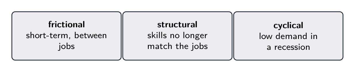
Three types of unemployment:
Frictional 摩擦性失业: between jobs or searching for a first job (normal, short).
Structural 结构性失业: skills or location don't match available jobs (technology, trade).
Cyclical 周期性失业: caused by a recession (a downturn in the business cycle).
Frictional + structural make up the natural rate of unemployment 自然失业率. At the natural rate cyclical unemployment is zero and the economy is at full employment 充分就业. The rate understates joblessness because it omits discouraged workers 灰心工人 and the underemployed.
Português
Uma longa fila de pessoas — desemprego são pessoas dispostas e capazes de trabalhar que não conseguem encontrar emprego
A força de trabalho 劳动力 são os empregados mais os desempregados (aqueles sem trabalho que buscam ativamente). Pessoas que não buscam não estão na força de trabalho.
Três tipos de desemprego: friccional, estrutural e cíclico
Exemplo resolvido. Um país tem $150$ milhões de empregados e $10$ milhão de desempregados (buscando ativamente), com $40$ milhões de adultos em idade working que não buscam. A força de trabalho é $150+10=160$ milhões, então a taxa de desemprego é $\dfrac{10}{160}=6.25\%$ e a taxa de participação é $\dfrac{160}{200}=80\%$.
Três tipos de desemprego:
Friccional 摩擦性失业: entre empregos ou buscando primeiro emprego (normal, curto).
Estrutural 结构性失业: habilidades ou localização não correspondem aos empregos disponíveis (tecnologia, comércio).
Cyclical 周期性失业: causado por uma recessão (uma desaceleração no ciclo econômico).
A friccional + estrutural compõem a taxa natural de desemprego 自然失业率. À taxa natural, o desemprego cíclico é zero e a economia está em pleno emprego 充分就业. A taxa subestima o desemprego porque omite trabalhadores desencorajados 灰心工人 e os subempregados.
natural rate of unemployment/ˈnætʃərəl reɪt ɒv ʌnemˈplɔɪmənt/
自然失业率
zì rán shī yè lǜ
full employment/fʊl emˈplɔɪmənt/
充分就业
chōng fèn jiù yè
discouraged workers/dɪˈskʌrɪdʒd ˈwɜːkəz/
灰心工人
huī xīn gōng rén
2.4
Índices de Preços e Inflação
Syllabus · Programa
English
Enduring Understanding (MEA-1): An economy's performance can be measured by different indicators such as gross domestic product (GDP), the inflation rate, and the unemployment rate.
Learning Objective MEA-1.F:
a. Define the consumer price index (CPI), inflation, deflation, disinflation, the inflation rate, and real variables.
b. Explain how price indices can be used to calculate the inflation rate and to compare nominal variables over time periods.
c. Calculate the CPI, the inflation rate, and changes in real variables.
MEA-1.F.1 The consumer price index (CPI) measures the change in income a consumer would need in order to maintain the same standard of living over time under a new set of prices as under the original set of prices.
MEA-1.F.2 The CPI measures the cost of a fixed basket of goods and services in a given year relative to the base year.
Exclusion statement: Calculating the producer price index (PPI) is beyond the scope of the course and AP Exam.
MEA-1.F.3 The inflation rate is determined by calculating the percentage change in a price index, such as CPI or the GDP deflator.
MEA-1.F.4 Real variables, such as real wages, are the nominal variables deflated by the price level.
Learning Objective MEA-1.G: Define the shortcomings of the CPI as a true measure of inflation.
MEA-1.G.1 The CPI as a measure of inflation has some shortcomings, such as substitution bias, causing it to overstate the true inflation rate.
Português
Compreensão Permanente (MEA-1): O desempenho de uma economia pode ser medido por diferentes indicadores, como Produto Interno Bruto (PIB), taxa de inflação e taxa de desemprego.
Objetivo de Aprendizagem MEA-1.F:
a. Definir o índice de preços ao consumidor (IPC), inflação, deflação, desinflação, a taxa de inflação e as variáveis reais.
b. Explicar como os índices de preços podem ser usados para calcular a taxa de inflação e comparar variáveis nominais entre períodos.
c. Calcular o IPC, a taxa de inflação e as mudanças nas variáveis reais.
MEA-1.F.1 O índice de preços ao consumidor (IPC) mede a mudança na renda que um consumidor precisaria para manter o mesmo padrão de vida ao longo do tempo sob um novo conjunto de preços em relação ao conjunto original de preços.
MEA-1.F.2 O IPC mede o custo de uma cesta fixa de bens e serviços em um ano dado em relação ao ano-base.
Declaração de exclusão: O cálculo do índice de preços ao produtor (IPP) está fora do escopo do curso e do Exame AP.
MEA-1.F.3 A taxa de inflação é determinada pelo cálculo da variação percentual em um índice de preços, como o IPC ou o deflator do PIB.
MEA-1.F.4 Variáveis reais, como salários reais, são as variáveis nominais deflacionadas pelo nível de preços.
Objetivo de Aprendizagem MEA-1.G: Definir as falhas do IPC como verdadeira medida de inflação.
MEA-1.G.1 O IPC como medida de inflação tem algumas falhas, como o viés de substituição, o que causa uma superestimação da taxa real de inflação.
Source: College Board AP Course and Exam Description · Fonte: College Board AP Course and Exam Description
English
Inflation 通货膨胀 is a sustained rise in the average price level. It is measured with a price index 价格指数, most often the consumer price index (CPI) 消费者价格指数, built from a fixed market basket of goods a typical household buys:
$$CPI=\frac{\text{cost of basket this year}}{\text{cost of basket in base year}}\times100.$$
The inflation rate is the percent change in the index between two years. Deflation 通货紧缩 is a falling price level; disinflation is a slowing of inflation.
Worked example. If the CPI is $200$ this year and was $190$ last year, the inflation rate is $\dfrac{200-190}{190}\times100\%=5.3\%$. A basket that cost $\$190$ then costs $\$200$ – the same goods, more dollars.
Português
A aisle de um supermercado: uma cesta fixa de bens mede a inflação através de um índice de preços
Inflação é um aumento sustentado no nível médio de preços. É medida com um índice de preços 价格指数, mais frequentemente o índice de preços ao consumidor (IPC) 消费者价格指数, construído a partir de uma cesta de mercado fixa de bens que uma família típica compra:
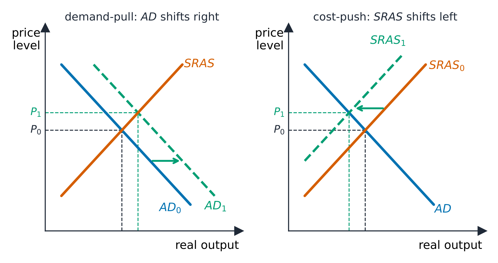
Inflação puxada por demanda e empurrada por custos no diagrama DA-OF
$$CPI=\frac{\text{cost of basket this year}}{\text{cost of basket in base year}}\times100.$$
A taxa de inflação é a variação percentual no índice entre dois anos. Deflação 通货紧缩 é um nível de preços em queda; desinflação é um desacelerar da inflação.
Exemplo resolvido. Se o IPC é $200$ este ano e era $190$ no ano passado, a taxa de inflação é $\dfrac{200-190}{190}\times100\%=5.3\%$. Um cesto que custava $\$190$ then costs $\$200$ – os mesmos bens, mais dólares.
Enduring Understanding (MEA-1): An economy's performance can be measured by different indicators such as gross domestic product (GDP), the inflation rate, and the unemployment rate.
Learning Objective MEA-1.H: Explain the costs that unexpected inflation (deflation) imposes on individuals and the economy.
MEA-1.H.1 Unexpected inflation arbitrarily redistributes wealth from one group of individuals to another group, such as lenders to borrowers.
Português
Compreensão Permanente (MEA-1): O desempenho de uma economia pode ser medido por diferentes indicadores, como Produto Interno Bruto (PIB), taxa de inflação e taxa de desemprego.
Objetivo de Aprendizagem MEA-1.H: Explicar os custos que a inflação inesperada (deflação) impõe aos indivíduos e à economia.
MEA-1.H.1 A inflação inesperada redistribui arbitrariamente a riqueza de um grupo de indivíduos para outro, como de credores para devedores.
Source: College Board AP Course and Exam Description · Fonte: College Board AP Course and Exam Description
English
Inflation redistributes and distorts:
It hurts lenders and savers and helps borrowers when it is unexpected, because loans are repaid in cheaper dollars. It erodes the value of money and fixed incomes.
Menu costs and uncertainty discourage investment.
Anticipated inflation is less harmful because contracts and interest rates adjust for it. This is why we separate nominal and real values.
Português
Inflation redistributes and distorts:
Prejudica credores e poupadores e ajuda devedores quando é inesperada, porque os empréstimos são reembolsados em dólares mais baratos. Erode o valor do dinheiro e dos rendimentos fixos.
Menu costs and uncertainty discourage investment.
A inflação antecipada é menos prejudicial porque contratos e taxas de juros se ajustam a ela. É por isso que separamos valores nominais e reais.
Enduring Understanding (MEA-1): An economy's performance can be measured by different indicators such as gross domestic product (GDP), the inflation rate, and the unemployment rate.
Learning Objective MEA-1.I: Define nominal GDP and real GDP.
MEA-1.I.1 Nominal GDP is a measure of how much is spent on output. Real GDP is a measure of how much is produced.
MEA-1.I.2 Nominal GDP measures aggregate output using current prices. Real GDP measures aggregate output using constant prices, thus removing the effect of changes in the overall price level.
Learning Objective MEA-1.J: Calculate real GDP and the GDP deflator.
MEA-1.J.1 One way of measuring real GDP is to weigh final goods and services by their prices in a base year. Because this can lead to overstatement of real GDP growth, statistical agencies actually use different methods.
MEA-1.J.2 Nominal GDP can be converted to real GDP by using the GDP deflator.
Português
Compreensão Permanente (MEA-1): O desempenho de uma economia pode ser medido por diferentes indicadores, como Produto Interno Bruto (PIB), taxa de inflação e taxa de desemprego.
Objetivo de Aprendizagem MEA-1.I: Definir o PIB nominal e o PIB real.
MEA-1.I.1 O PIB nominal é uma medida do quanto é gasto com a produção. O PIB real é uma medida do quanto é produzido.
MEA-1.I.2 O PIB nominal mede a produção agregada usando preços correntes. O PIB real mede a produção agregada usando preços constantes, eliminando assim o efeito das mudanças no nível geral de preços.
Objetivo de Aprendizagem MEA-1.J: Calcular o PIB real e o deflator do PIB.
MEA-1.J.1 Uma maneira de medir o PIB real é ponderar os bens finais e serviços pelos seus preços em um ano-base. Como isso pode levar a uma superestimação do crescimento do PIB real, as agências estatísticas usam na verdade métodos diferentes.
MEA-1.J.2 O PIB nominal pode ser convertido em PIB real usando o deflator do PIB.
Source: College Board AP Course and Exam Description · Fonte: College Board AP Course and Exam Description
English
Nominal GDP 名义GDP is valued at current prices, so it rises with both output and prices.
Real GDP 实际GDP is valued at constant (base-year) prices, stripping out inflation, so it reflects true output. Real GDP is the honest measure of growth.
Worked example. Nominal GDP is $\$22$ trillion and the GDP deflator is $110$. Real GDP is $\dfrac{22}{110}\times100=\$20$ trillion. The extra $\$2$ trillion of nominal GDP is pure price rise, not real output – which is why growth is always measured with real GDP.
Exam skill: be fluent converting nominal to real using a price index, and computing an inflation rate or a growth rate as a percent change.
Português
PIB nominal é avaliado a preços atuais, pelo que sobe tanto com a produção como com os preços.
PIB real é avaliado a preços constantes (do ano-base), eliminando a inflação, pelo que reflete a produção verdadeira. O PIB real é a medida honesta do crescimento.
Exemplo resolvido. O PIB nominal é $\$22$ trillion and the GDP deflator is $110$. Real GDP is $\dfrac{22}{110}\times100=\$20$ triliões. Os $\$2$ triliões extras de PIB nominal são apenas um aumento de preços, não de produção real – é por isso que o crescimento é sempre medido com o PIB real.
Habilidade de exame: seja fluente na conversão de nominal para real usando um índice de preços, e no cálculo de uma taxa de inflação ou de uma taxa de crescimento como uma variação percentual.
consumer price index (CPI)/kənˈsuːmə praɪs ˈɪndeks/
消费者价格指数
xiāo fèi zhě jià gé zhǐ shù
Deflation/diːˈfleɪʃn/
通货紧缩
tōng huò jǐn suō
Nominal GDP/ˈnɒmɪnl ˌdʒiː diː ˈpiː/
名义
míng yì
Real GDP/rɪəl ˌdʒiː diː ˈpiː/
实际
shí jì
2.7
Ciclos Econômicos
Syllabus · Programa
English
Enduring Understanding (MEA-2): The economy fluctuates between periods of expansion and contraction in the short run, but economic growth can occur in the long run.
Learning Objective MEA-2.A:
a. Define (using graphs and data as appropriate) turning points and phases of the business cycle.
b. Explain (using graphs and data as appropriate) turning points and phases of the business cycle.
MEA-2.A.1 Business cycles are fluctuations in aggregate output and employment because of changes in aggregate supply and/or aggregate demand.
MEA-2.A.2 The phases of a business cycle are recession and expansion.
MEA-2.A.3 The turning points of a business cycle are peak and trough.
MEA-2.A.4 The difference between actual output and potential output is the output gap.
MEA-2.A.5 Potential output is also called full-employment output. It is the level of GDP where unemployment is equal to the natural rate of unemployment. [See EK MEA-1.E.2]
Português
Entendimento Duradouro (MEA-2): A economia flutua entre períodos de expansão e contração no curto prazo, mas o crescimento econômico pode ocorrer no longo prazo.
Objetivo de Aprendizagem MEA-2.A:
a. Definir (usando gráficos e dados, conforme apropriado) pontos de virada e fases do ciclo empresarial.
b. Explicar (usando gráficos e dados, conforme apropriado) pontos de virada e fases do ciclo empresarial.
MEA-2.A.1 Ciclos empresariais são flutuações na produção agregada e no emprego devido a mudanças na oferta agregada e/ou demanda agregada.
MEA-2.A.2 As fases de um ciclo empresarial são recessão e expansão.
MEA-2.A.3 Os pontos de virada de um ciclo empresarial são pico e vale.
MEA-2.A.4 A diferença entre a produção real e a produção potencial é o hiato de produção.
MEA-2.A.5 A produção potencial também é chamada de produção de pleno emprego. É o nível de PIB onde o desemprego é igual à taxa natural de desemprego. [Ver EK MEA-1.E.2]
Source: College Board AP Course and Exam Description · Fonte: College Board AP Course and Exam Description
English
The business cycle
The business cycle 经济周期 is the economy's short-run ups and downs in real GDP around its long-run growth trend: expansion 扩张 (rising output, falling unemployment) up to a peak 顶峰, then contraction/recession 衰退 (falling output, rising cyclical unemployment) down to a trough 谷底, then recovery. A recession is commonly two consecutive quarters of falling real GDP. Unemployment and inflation move roughly opposite over the cycle – the tension the rest of the course tries to manage.
Português
The business cycle
O ciclo económico 经济周期 são as oscilações de curto prazo da economia no PIB real em torno da sua tendência de crescimento de longo prazo: expansão 扩张 (produção crescente, desemprego decrescente) até um pico 顶峰, depois contração/recessão 衰退 (produção decrescente, aumento do desemprego cíclico) até um vale 谷底, depois recuperação. Uma recessão é comumente dois trimestres consecutivos de queda do PIB real. Desemprego e inflação movem-se aproximadamente em direções opostas ao longo do ciclo – a tensão que o resto do curso tenta gerir.
O PIB real oscilando em torno de sua tendência de longo prazo
Compute GDP by the expenditure method $C+I+G+X_n$ and count only final goods (avoid double counting).
Unemployment rate = unemployed ÷ labor force; discouraged workers leave the labor force (so the rate can understate joblessness).
Know the three unemployment types (frictional, structural, cyclical) and that the natural rate excludes cyclical.
Inflation is the % change in the CPI; convert nominal to real with a price index and always use real GDP for growth.
Place events on the business cycle (expansion → peak → contraction → trough).
Português
Calcule o PIB pelo método da despesa $C+I+G+X_n$ e conte apenas os bens finais (evite a dupla contagem).
Taxa de desemprego = desempregados ÷ força de trabalho; os trabalhadores desencorajados saem da força de trabalho (por isso a taxa pode subestimar o desemprego).
Conheça os três tipos de desemprego (friccional, estrutural, cíclico) e que a taxa natural exclui o cíclico.
A inflação é a % de variação no IPC; converta nominal para real com um índice de preços e use sempre o PIB real para o crescimento.
Coloque os eventos no ciclo económico (expansão → pico → contração → vale).
Enduring Understanding (MOD-2): Economists use the aggregate demand–aggregate supply model to represent the relationship between the price level and aggregate output in an economy and to illustrate how output, employment, and the price level respond to macroeconomic shocks.
Learning Objective MOD-2.A:
a. Define (using graphs as appropriate) the aggregate demand (AD) curve.
b. Explain (using graphs as appropriate) the slope of the AD curve and its determinants.
MOD-2.A.1 The aggregate demand (AD) curve describes the relationship between the price level and the quantity of goods and services demanded by households (consumption), firms (investment), government (government spending), and the rest of the world (net exports).
MOD-2.A.2 The negative slope of the AD curve is explained by the real wealth effect, the interest rate effect, and the exchange rate effect. [See EK MKT-3.A.1]
MOD-2.A.3 Any change in the components of aggregate demand (consumption, investment, government spending, or net exports) that is not due to changes in the price level leads to a shift of the AD curve.
Português
Entendimento Duradouro (MOD-2): Os economistas usam o modelo de demanda agregada–oferta agregada para representar a relação entre o nível de preços e a produção agregada em uma economia e para ilustrar como a produção, o emprego e o nível de preços respondem a choques macroeconômicos.
Objetivo de Aprendizagem MOD-2.A:
a. Definir (usando gráficos, conforme apropriado) a curva de demanda agregada (DA).
b. Explicar (usando gráficos, conforme apropriado) a inclinação da curva DA e seus determinantes.
MOD-2.A.1 A curva de demanda agregada (DA) descreve a relação entre o nível de preços e a quantidade de bens e serviços demandados pelas famílias (consumo), empresas (investimento), governo (gastos governamentais) e pelo resto do mundo (exportações líquidas).
MOD-2.A.2 A inclinação negativa da curva DA é explicada pelo efeito da riqueza real, pelo efeito da taxa de juros e pelo efeito cambial. [Ver EK MKT-3.A.1]
MOD-2.A.3 Qualquer mudança nos componentes da demanda agregada (consumo, investimento, gastos governamentais ou exportações líquidas) que não seja devida a mudanças no nível de preços leva a um deslocamento da curva DA.
Source: College Board AP Course and Exam Description · Fonte: College Board AP Course and Exam Description
English
The AD–AS model: a demand shock
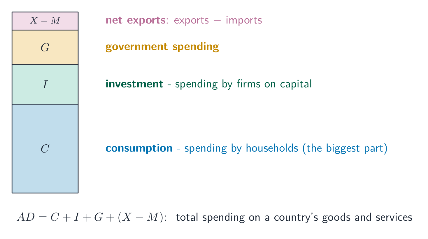
Aggregate demand (AD) 总需求 shows the total quantity of real output ($C+I+G+X_n$) buyers want at each price level 价格水平. It slopes downward for three reasons special to the whole economy:
the wealth effect 财富效应 (a higher price level shrinks the real value of money, so people buy less),
the interest-rate effect 利率效应 (a higher price level raises money demand and interest rates, cutting investment),
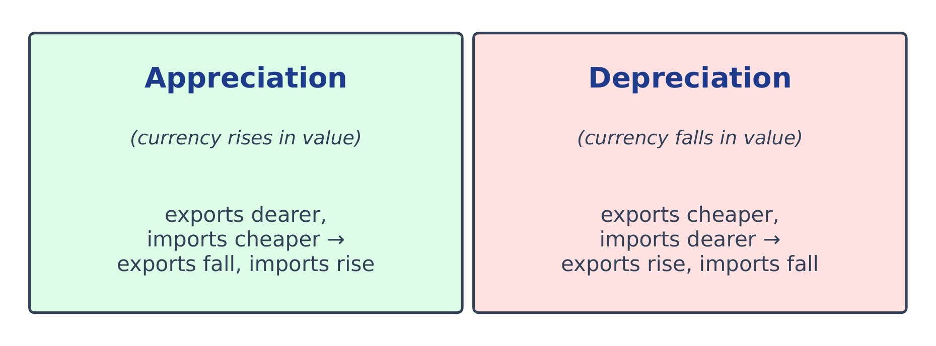
the net-export effect (a higher domestic price level makes exports dearer and imports cheaper).
A change in the price level is a movement along AD. AD shifts when any component of $C+I+G+X_n$ changes for another reason – consumer confidence, business expectations, government spending, taxes, or foreign incomes.
Português
Uma skyline urbana: a produção nacional e a procura agregada refletem a despesa em toda a economiaO modelo DA-AS: um choque de demanda
Procura agregada (PA) mostra a quantidade total de produção real ($C+I+G+X_n$) que os compradores desejam a cada nível de preços. Ela inclina-se para baixo por três razões especiais para toda a economia:
A procura agregada é a despesa total: consumo, investimento, governo e exportações líquidas
o efeito riqueza (um nível de preços mais alto reduz o valor real do dinheiro, por isso as pessoas compram menos),
o efeito taxa de juro (um nível de preços mais alto aumenta a procura de dinheiro e as taxas de juro, cortando o investimento),
o efeito exportações líquidas (um nível de preços doméstico mais alto torna as exportações mais caras e as importações mais baratas).
Uma mudança no nível de preços é um movimento ao longo da PA. A PA desloca-se quando qualquer componente de $C+I+G+X_n$ muda por outra razão – confiança dos consumidores, expectativas empresariais, gastos do governo, impostos ou rendimentos estrangeiros.
3.2
The Spending and Tax Multipliers
Syllabus · Programa
English
Enduring Understanding (MOD-2): Economists use the aggregate demand–aggregate supply model to represent the relationship between the price level and aggregate output in an economy and to illustrate how output, employment, and the price level respond to macroeconomic shocks.
Learning Objective MOD-2.B:
a. Define the expenditure multiplier, the tax multiplier, the marginal propensity to consume, and the marginal propensity to save.
b. Explain how changes in spending and taxes lead to changes in real GDP.
c. Calculate how changes in spending and taxes lead to changes in real GDP.
MOD-2.B.1 A $\$1$ change to autonomous expenditures leads to further changes in total expenditures and total output.
MOD-2.B.2 The expenditure multiplier quantifies the size of the change in aggregate demand as a result of a change in any of the components of aggregate demand.
MOD-2.B.3 The tax multiplier quantifies the size of the change in aggregate demand as a result of a change in taxes.
MOD-2.B.4 The expenditure multiplier and tax multiplier depend on the marginal propensity to consume.
MOD-2.B.5 The marginal propensity to consume is the change in consumer spending divided by the change in disposable income. The sum of the marginal propensity to consume and marginal propensity to save is equal to one.
Português
Entendimento Duradouro (MOD-2): Os economistas usam o modelo de demanda agregada–oferta agregada para representar a relação entre o nível de preços e a produção agregada em uma economia e para ilustrar como a produção, o emprego e o nível de preços respondem a choques macroeconômicos.
Objetivo de Aprendizagem MOD-2.B:
a. Definir o multiplicador de despesas, o multiplicador fiscal, a propensão marginal a consumir e a propensão marginal a poupar.
b. Explicar como mudanças em gastos e impostos levam a mudanças no PIB real.
c. Calcular como mudanças em gastos e impostos levam a mudanças no PIB real.
MOD-2.B.1 Um $\$1$ de mudança nas despesas autônomas leva a outras mudanças nas despesas totais e na produção total.
MOD-2.B.2 O multiplicador de despesas quantifica a magnitude da mudança na demanda agregada como resultado de uma mudança em qualquer um dos componentes da demanda agregada.
MOD-2.B.3 O multiplicador fiscal quantifica a magnitude da mudança na demanda agregada como resultado de uma mudança em impostos.
MOD-2.B.4 O multiplicador de despesas e o multiplicador fiscal dependem da propensão marginal a consumir.
MOD-2.B.5 A propensão marginal a consumir é a mudança no consumo dividida pela mudança na renda disponível. A soma da propensão marginal a consumir e da propensão marginal a poupar é igual a um.
Source: College Board AP Course and Exam Description · Fonte: College Board AP Course and Exam Description
English
The spending multiplier
A change in spending sets off further rounds of spending, so the final change in GDP is larger than the initial change – the multiplier effect 乘数效应. It depends on the marginal propensity to consume 边际消费倾向 (MPC), the fraction of extra income that is spent (the rest is the marginal propensity to save 边际储蓄倾向, MPS, with $MPC+MPS=1$):
The tax multiplier is smaller in size and negative (a tax cut raises GDP; a tax rise lowers it). Total change in GDP $=$ (multiplier) $\times$ (initial change).
Worked example. If $MPC=0.8$, the spending multiplier is $\dfrac{1}{1-0.8}=5$, so a $\$10$ billion rise in government spending lifts real GDP by $5\times\$10=\$50$ billion. The tax multiplier is $-\dfrac{0.8}{0.2}=-4$, so a $\$10$ billion tax cut raises GDP by only $\$40$ billion – weaker, because part of the tax cut is saved.
Exam skill: compute both multipliers from the MPC and find the resulting change in real GDP – an almost-guaranteed calculation.
Português
The spending multiplier
Uma mudança nos gastos desencadeia novas rodadas de gastos, pelo que a mudança final no PIB é maior do que a mudança inicial – o efeito multiplicador 乘数效应. Depende da propensão marginal a consumir 边际消费倾向 (MPC), a fração da renda extra que é gasta (o restante é a propensão marginal a poupar 边际储蓄倾向, MPS, com $MPC+MPS=1$):
Uma injeção multiplica-se num aumento global maior da renda
O multiplicador fiscal é menor em tamanho e negativo (um corte nos impostos aumenta o PIB; um aumento dos impostos diminui-o). Mudança total no PIB $=$ (multiplicador) $\times$ (mudança inicial).
Exemplo resolvido. Se $MPC=0.8$, o multiplicador de gastos é $\dfrac{1}{1-0.8}=5$, logo um corte nos impostos de $\$10$ billion rise in government spending lifts real GDP by $5\times\$10=\$50$ billion. The tax multiplier is $-\dfrac{0.8}{0.2}=-4$, so a $\$10$ bilhões eleva o PIB apenas em $\$40$ bilhões – mais fraco, porque parte do corte nos impostos é poupado.
Habilidade de exame: calcule ambos os multiplicadores a partir da PIM e encontre a mudança resultante no PIB real – um cálculo quase garantido.
Explore · Explorar
Veja o multiplicador de gastos se propagar
Um dólar de novos gastos torna-se a renda de alguém, parte da qual eles gastam novamente — então o efeito total é um multiplicador da primeira injeção, determinado pela propensão marginal a consumir (PMC).
3.3
Short-Run Aggregate Supply
Syllabus · Programa
English
Enduring Understanding (MOD-2): Economists use the aggregate demand–aggregate supply model to represent the relationship between the price level and aggregate output in an economy and to illustrate how output, employment, and the price level respond to macroeconomic shocks.
Learning Objective MOD-2.C:
a. Define (using graphs as appropriate) the short-run aggregate supply (SRAS) curve.
b. Explain (using graphs as appropriate) the slope of the SRAS curve and its determinants.
MOD-2.C.1 The short-run aggregate supply (SRAS) curve describes the relationship between the price level and the quantity of goods and services supplied in an economy.
MOD-2.C.2 The SRAS curve is upward-sloping because of sticky wages and prices. [See EK MOD-2.E.1]
MOD-2.C.3 Any factor that causes production costs to change, such as a change in inflationary expectations, will cause the SRAS curve to shift.
Learning Objective MOD-2.D: Explain (using graphs as appropriate) how movement along the SRAS curve implies a relationship between the price level (and inflation) and unemployment.
MOD-2.D.1 Moving along the SRAS curve, an increase in the price level is associated with an increase in output, which means employment must correspondingly rise. With the labor force held constant, unemployment will fall. So, there is a short-run trade-off between inflation and unemployment. [See EK MOD-3.A.1]
Português
Entendimento Duradouro (MOD-2): Os economistas usam o modelo de demanda agregada–oferta agregada para representar a relação entre o nível de preços e a produção agregada em uma economia e para ilustrar como a produção, o emprego e o nível de preços respondem a choques macroeconômicos.
Objetivo de Aprendizagem MOD-2.C:
a. Definir (usando gráficos, conforme apropriado) a curva de oferta agregada de curto prazo (OACP).
b. Explicar (usando gráficos, conforme apropriado) a inclinação da curva OACP e seus determinantes.
MOD-2.C.1 A curva de oferta agregada de curto prazo (OACP) descreve a relação entre o nível de preços e a quantidade de bens e serviços ofertados em uma economia.
MOD-2.C.2 A curva OACP tem inclinação ascendente devido a salários e preços rígidos. [Ver EK MOD-2.E.1]
MOD-2.C.3 Qualquer fator que cause mudanças nos custos de produção, como uma mudança nas expectativas inflacionárias, fará com que a curva OACP se desloque.
Objetivo de Aprendizagem MOD-2.D: Explicar (usando gráficos, conforme apropriado) como o movimento ao longo da curva OACP implica uma relação entre o nível de preços (e inflação) e o desemprego.
MOD-2.D.1 Ao longo da curva OACP, um aumento no nível de preços está associado a um aumento na produção, o que significa que o emprego deve aumentar correspondentemente. Com a força de trabalho mantida constante, o desemprego cairá. Portanto, há um trade-off de curto prazo entre inflação e desemprego. [Ver EK MOD-3.A.1]
Source: College Board AP Course and Exam Description · Fonte: College Board AP Course and Exam Description
English
Short-run aggregate supply (SRAS) 短期总供给 slopes upward: in the short run some input prices (especially nominal wages 名义工资) are sticky 粘性, so a higher output price level widens profit margins and firms produce more. SRAS shifts with input prices, productivity, taxes/subsidies on producers, and supply shocks (e.g. an oil-price change). A rise in input costs shifts SRAS left.
Português
Uma central elétrica e um site industrial: a oferta agregada de curto prazo depende dos custos de produção
Oferta agregada de curto prazo (OAS) inclina-se para cima: no curto prazo alguns preços de inputs (especialmente salários nominais) são pegajosos, por isso um nível de preços de output mais alto alarga as margens de lucro e as firmas produzem mais. A OAS desloca-se com preços de inputs, produtividade, impostos/subvenções aos produtores e choques de oferta (por exemplo, uma mudança no preço do petróleo). Um aumento nos custos de input desloca a OAS para a esquerda.
3.4
Long-Run Aggregate Supply
Syllabus · Programa
English
Enduring Understanding (MOD-2): Economists use the aggregate demand–aggregate supply model to represent the relationship between the price level and aggregate output in an economy and to illustrate how output, employment, and the price level respond to macroeconomic shocks.
Learning Objective MOD-2.E: Define (using graphs as appropriate) the short run and the long run.
MOD-2.E.1 In the long run all prices and wages are fully flexible, while in the short run some input prices are fixed. A consequence of flexible long-run prices and wages is the lack of a long-run trade-off between inflation and unemployment.
Learning Objective MOD-2.F: Define (using graphs as appropriate) the long-run aggregate supply (LRAS) curve.
MOD-2.F.1 The LRAS curve corresponds to the production possibilities curve (PPC) because they both represent maximum sustainable capacity. Maximum sustainable capacity is the total output an economic system will produce over a set period of time if all resources are fully employed. [See LO MOD-2.I]
MOD-2.F.2 The LRAS curve is vertical at the full-employment level of output because in the long run wages and prices fully adjust.
Português
Entendimento Duradouro (MOD-2): Os economistas usam o modelo de demanda agregada–oferta agregada para representar a relação entre o nível de preços e a produção agregada em uma economia e para ilustrar como a produção, o emprego e o nível de preços respondem a choques macroeconômicos.
Objetivo de Aprendizagem MOD-2.E: Definir (usando gráficos, conforme apropriado) o curto prazo e o longo prazo.
MOD-2.E.1 No longo prazo, todos os preços e salários são totalmente flexíveis, enquanto no curto prazo alguns preços de insumos são fixos. Consequência dos preços e salários flexíveis de longo prazo é a falta de um trade-off de longo prazo entre inflação e desemprego.
Objetivo de Aprendizagem MOD-2.F: Definir (usando gráficos, conforme apropriado) a curva de oferta agregada de longo prazo (OALP).
MOD-2.F.1 A curva OALP corresponde à curva de possibilidades de produção (CPP) porque ambas representam capacidade máxima sustentável. Capacidade máxima sustentável é a produção total que um sistema econômico produzirá durante um período específico se todos os recursos estiverem plenamente empregados. [Ver LO MOD-2.I]
MOD-2.F.2 A curva OALP é vertical no nível de produção de pleno emprego porque, no longo prazo, salários e preços se ajustam completamente.
Source: College Board AP Course and Exam Description · Fonte: College Board AP Course and Exam Description
English
Long-run aggregate supply (LRAS) 长期总供给 is vertical at the economy's full-employment (potential) output 潜在产出$Y_f$. In the long run all prices and wages are fully flexible (only in the short run are some input prices fixed), so output depends only on real factors – resources, technology, institutions – not the price level. LRAS shifts only with economic growth (more or better resources). LRAS corresponds to the production possibilities curve (PPC) 生产可能性曲线: both mark the economy's maximum sustainable capacity, so an outward LRAS shift and an outward PPC shift are the same event drawn two ways. The vertical LRAS is why, in the long run, demand policy changes prices, not output.
Português
A oferta agregada de longo prazo (LRAS) 长期总供给 é vertical na produção de pleno emprego (potencial) 潜在产出 da economia $Y_f$. No longo prazo, todos os preços e salários são totalmente flexíveis (só no curto prazo alguns preços de insumos são fixos), pelo que a produção depende apenas de fatores reais – recursos, tecnologia, instituições –, e não do nível de preços. A LRAS muda apenas com crescimento económico (mais ou melhores recursos). A LRAS corresponde à curva de possibilidades de produção (PPC) 生产可能性曲线: ambas marcam a capacidade sustentável máxima da economia, pelo que um deslocamento externo da LRAS e um deslocamento externo da PPC são o mesmo evento desenhado de duas formas. É a LRAS vertical que explica por que, no longo prazo, as políticas de demanda alteram os preços, não a produção.
Política do lado da oferta desloca a oferta agregada de longo prazo para a direita: mais output, preços mais baixos
3.5
Equilíbrio no Modelo AD-AS
Syllabus · Programa
English
Enduring Understanding (MOD-2): Economists use the aggregate demand–aggregate supply model to represent the relationship between the price level and aggregate output in an economy and to illustrate how output, employment, and the price level respond to macroeconomic shocks.
Learning Objective MOD-2.G: Explain (using graphs as appropriate) the short-run and long-run equilibrium price level and output level.
MOD-2.G.1 Short-run equilibrium occurs when the aggregate quantity of output demanded and the aggregate quantity of output supplied are equal—i.e., at the intersection of the AD and SRAS curves.
MOD-2.G.2 Long-run equilibrium occurs when the AD and SRAS curves intersect on the LRAS—i.e., at the full-employment level of real output.
MOD-2.G.3 The short-run equilibrium output can be at the full-employment level of output, above it, or below it, creating positive (i.e., inflationary) or negative (i.e., recessionary) output gaps.
Português
Entendimento Duradouro (MOD-2): Os economistas usam o modelo de demanda agregada–oferta agregada para representar a relação entre o nível de preços e a produção agregada em uma economia e para ilustrar como a produção, o emprego e o nível de preços respondem a choques macroeconômicos.
Objetivo de Aprendizagem MOD-2.G: Explicar (usando gráficos, conforme apropriado) o nível de preços e de produção de equilíbrio de curto e longo prazo.
MOD-2.G.1 O equilíbrio de curto prazo ocorre quando a quantidade agregada de produção demandada e a quantidade agregada de produção ofertada são iguais—isto é, na interseção das curvas DA e OACP.
MOD-2.G.2 O equilíbrio de longo prazo ocorre quando as curvas DA e OACP se intersectam na OALP—isto é, no nível de produção real de pleno emprego.
MOD-2.G.3 A produção de equilíbrio de curto prazo pode estar no nível de produção de pleno emprego, acima dele ou abaixo dele, criando hiatos positivos (ou seja, inflacionários) ou negativos (ou seja, recessivos).
Source: College Board AP Course and Exam Description · Fonte: College Board AP Course and Exam Description
English
The economy settles where AD meets SRAS, fixing the equilibrium price level and real GDP. Comparing that output to $Y_f$ (the LRAS line) gives the economy's state:
output $: a recessionary gap 衰退缺口 (cyclical unemployment),
output $>Y_f$: an inflationary gap 通胀缺口 (overheating),
output $=Y_f$: long-run equilibrium.
Português
A economia estabiliza onde AD encontra SRAS, fixando o nível de preços de equilíbrio e o PIB real. Comparando essa produção com $Y_f$ (a linha LRAS) dá-nos o estado da economia:
Macroeconomic equilibrium where aggregate demand meets aggregate supply
output $: a recessionary gap 衰退缺口 (cyclical unemployment),
output $>Y_f$: an inflationary gap 通胀缺口 (overheating),
output $=Y_f$: long-run equilibrium.
Explore · Explorar
Encontre o equilíbrio no modelo AD-AS
Demanda agregada e oferta agregada se cruzam no nível de preços e no PIB real da economia. Um choque de demanda ou oferta desloca uma curva e move a produção e os preços de toda a economia.
production possibilities curve (PPC)/prəˈdʌkʃn ˌpɒsəˈbɪlɪtiz kɜːv/
生产可能性曲线
shēng chǎn kě néng xìng qū xiàn
recessionary gap/rɪˈseʃənəri ɡæp/
衰退缺口
shuāi tuì quē kǒu
inflationary gap/ɪnˈfleɪʃənəri ɡæp/
通胀缺口
tōng zhàng quē kǒu
stagflation/stæɡˈfleɪʃn/
滞胀
zhì zhàng
3.6
Short-Run Changes: Demand and Supply Shocks
Syllabus · Programa
English
Enduring Understanding (MOD-2): Economists use the aggregate demand–aggregate supply model to represent the relationship between the price level and aggregate output in an economy and to illustrate how output, employment, and the price level respond to macroeconomic shocks.
Learning Objective MOD-2.H: Explain (using graphs as appropriate) the response of output, employment, and the price level to an aggregate demand or aggregate supply shock in the short run.
MOD-2.H.1 A positive (negative) shock in AD causes output, employment, and the price level to rise (fall) in the short run.
MOD-2.H.2 A positive (negative) shock in SRAS causes output and employment to rise (fall) and the price level to fall (rise) in the short run.
MOD-2.H.3 Inflation can be caused by changes in aggregate demand (demand-pull) or aggregate supply (cost-push).
Português
Entendimento Duradouro (MOD-2): Os economistas usam o modelo de demanda agregada–oferta agregada para representar a relação entre o nível de preços e a produção agregada em uma economia e para ilustrar como a produção, o emprego e o nível de preços respondem a choques macroeconômicos.
Objetivo de Aprendizagem MOD-2.H: Explicar (usando gráficos, quando apropriado) a resposta da produção, do emprego e do nível de preços a um choque na demanda agregada ou na oferta agregada no curto prazo.
MOD-2.H.1 Um choque positivo (negativo) na AD causa aumento (redução) na produção, no emprego e no nível de preços no curto prazo.
MOD-2.H.2 Um choque positivo (negativo) na SRAS causa aumento (redução) na produção e no emprego e redução (aumento) no nível de preços no curto prazo.
MOD-2.H.3 A inflação pode ser causada por mudanças na demanda agregada (puxada pela demanda) ou na oferta agregada (impulsionada pelos custos).
Source: College Board AP Course and Exam Description · Fonte: College Board AP Course and Exam Description
English
A demand shock shifts AD: a positive one (more spending) raises both price level and output (and lowers unemployment); a negative one lowers both.
A supply shock shifts SRAS: a negative one (higher input costs) raises the price level and lowers output at once – stagflation 滞胀 – the hardest case for policymakers, because fixing one worsens the other.
Português
Um choque de demanda desloca a AD: um choque positivo (mais gastos) eleva tanto o nível de preços quanto a produção (e reduz o desemprego); um choque negativo reduz ambos.
Um choque de oferta desloca SRAS: um choque negativo (custos de insumos mais altos) aumenta o nível de preços e baixa a produção simultaneamente – estagflação 滞胀 – o caso mais difícil para os políticos, pois corrigir um piora o outro.
3.7
Autoajustamento de Longo Prazo
Syllabus · Programa
English
Enduring Understanding (MOD-2): Economists use the aggregate demand–aggregate supply model to represent the relationship between the price level and aggregate output in an economy and to illustrate how output, employment, and the price level respond to macroeconomic shocks.
Learning Objective MOD-2.I: Explain (using graphs as appropriate) the response of output, employment, and the price level to an aggregate demand or aggregate supply shock in the long run.
MOD-2.I.1 In the long run, in the absence of government policy actions, flexible wages and prices will adjust to restore full employment and unemployment will revert to its natural rate after a shock to aggregate demand or short-run aggregate supply. [See EK MEA-1.E.2]
MOD-2.I.2 Shifts in the long-run aggregate supply curve indicate changes in the full-employment level of output and economic growth.
Português
Entendimento Duradouro (MOD-2): Os economistas usam o modelo de demanda agregada–oferta agregada para representar a relação entre o nível de preços e a produção agregada em uma economia e para ilustrar como a produção, o emprego e o nível de preços respondem a choques macroeconômicos.
Objetivo de Aprendizagem MOD-2.I: Explicar (usando gráficos, quando apropriado) a resposta da produção, do emprego e do nível de preços a um choque na demanda agregada ou na oferta agregada no longo prazo.
MOD-2.I.1 No longo prazo, na ausência de ações governamentais, salários e preços flexíveis se ajustarão para restaurar o pleno emprego e o desemprego retornará à sua taxa natural após um choque na demanda agregada ou na oferta agregada de curto prazo. [Ver EK MEA-1.E.2]
MOD-2.I.2 Deslocamentos na curva de oferta agregada de longo prazo indicam mudanças no nível de plena ocupação da produção e no crescimento econômico.
Source: College Board AP Course and Exam Description · Fonte: College Board AP Course and Exam Description
English
Left alone, the economy self-corrects through flexible wages:
In a recessionary gap, high unemployment eventually pushes nominal wages down, shifting SRAS right until output returns to $Y_f$ at a lower price level.
In an inflationary gap, labor shortages push wages up, shifting SRAS left back to $Y_f$ at a higher price level.
The debate over how fast this happens is the case for (or against) active policy: self-adjustment is slow and painful, which is the argument for intervening.
Português
Deixado por si só, a economia se autorregula através de salários flexíveis:
Em um gap recessivo, o alto desemprego eventualmente empurra os salários nominais para baixo, deslocando a ASL para a direita até que a produção retorne a $Y_f$ em um nível de preços mais baixo.
Em um gap inflacionário, a escassez de mão de obra empurra os salários para cima, deslocando a ASL para a esquerda de volta para $Y_f$ em um nível de preços mais alto.
O debate sobre quão rápido isso acontece é o argumento a favor (ou contra) da política ativa: o autoajuste é lento e doloroso, o que é o argumento para intervir.
3.8
Política Fiscal
Syllabus · Programa
English
Enduring Understanding (POL-1): Fiscal and monetary policy have short-run effects on macroeconomic outcomes.
Learning Objective POL-1.A:
a. Define fiscal policy and related terms.
b. Explain (using graphs as appropriate) the short-run effects of a fiscal policy action.
c. Calculate the short-run effects of a fiscal policy action.
POL-1.A.1 Governments implement fiscal policies to achieve macroeconomic goals, such as full employment.
POL-1.A.2 The tools of fiscal policy are government spending and taxes/transfers.
POL-1.A.3 Changes in government spending affect aggregate demand directly, and changes in taxes/transfers affect aggregate demand indirectly.
POL-1.A.4 The government spending multiplier is greater than the tax multiplier.
POL-1.A.5 Expansionary or contractionary fiscal policies are used to restore full employment when the economy is in a negative (i.e., recessionary) or positive (i.e., inflationary) output gap.
POL-1.A.6 Fiscal policy can influence aggregate demand, real output, and the price level. [See also EK MKT-5.E.2 for the effect on exchange rates.]
POL-1.A.7 The AD–AS model is used to demonstrate the short-run effects of fiscal policy.
Learning Objective POL-1.B: Define why there are lags to discretionary fiscal policy.
POL-1.B.1 In reality, there are lags to discretionary fiscal policy because of factors such as the time it takes to decide on and implement a policy action.
Português
Compreensão Permanente (POL-1): As políticas fiscal e monetária têm efeitos de curto prazo sobre os resultados macroeconômicos.
Objetivo de Aprendizagem POL-1.A:
a. Definir política fiscal e termos relacionados.
b. Explicar (usando gráficos, quando apropriado) os efeitos de curto prazo de uma ação de política fiscal.
c. Calcular os efeitos de curto prazo de uma ação de política fiscal.
POL-1.A.1 Os governos implementam políticas fiscais para alcançar objetivos macroeconômicos, como o pleno emprego.
POL-1.A.2 As ferramentas da política fiscal são gastos públicos e impostos/transferências.
POL-1.A.3 Alterações nos gastos públicos afetam a demanda agregada diretamente, e alterações em impostos/transferências afetam a demanda agregada indiretamente.
POL-1.A.4 O multiplicador dos gastos públicos é maior que o multiplicador tributário.
POL-1.A.5 Políticas fiscais expansivas ou contrativas são usadas para restaurar o pleno emprego quando a economia está com um hiato negativo (ou seja, recessivo) ou positivo (ou seja, inflacionário).
POL-1.A.6 A política fiscal pode influenciar a demanda agregada, a produção real e o nível de preços. [Ver também EK MKT-5.E.2 para o efeito sobre as taxas de câmbio.]
POL-1.A.7 O modelo AD–AS é usado para demonstrar os efeitos de curto prazo da política fiscal.
Objetivo de Aprendizagem POL-1.B: Definir por que existem defasagens na política fiscal discricionária.
POL-1.B.1 Na realidade, há defasagens na política fiscal discricionária devido a fatores como o tempo necessário para decidir e implementar uma ação de política.
Source: College Board AP Course and Exam Description · Fonte: College Board AP Course and Exam Description
English
Fiscal policy 财政政策 is the government's use of spending and taxes to shift AD:
Expansionary 扩张性 (more spending or lower taxes) shifts AD right to close a recessionary gap.
Contractionary 紧缩性 (less spending or higher taxes) shifts AD left to close an inflationary gap.
Size the policy with the multipliers: to close a gap of a given size, the required change in spending is (gap) $\div$ (spending multiplier). Limits include time lags, crowding out (below), and political difficulty.
Worked example. An economy has a $\$100$ billion recessionary gap and $MPC=0.75$ (spending multiplier $=\dfrac{1}{0.25}=4$). To close it, the government must raise spending by $\dfrac{\$100\text{ billion}}{4}=\$25$ billion. Using a tax cut instead (tax multiplier $-3$) would require a larger $\dfrac{100}{3}\approx\$33$ billion cut.
Exam skill: you must draw the correctly labeled AD-AS graph, identify the gap, prescribe the right fiscal action and its direction, and often calculate the exact spending or tax change needed.
Português
Política fiscal 财政政策 é o uso pelo governo de gastos e impostos para deslocar a AD:
A política fiscal expansionista desloca a AD para a direita, aumentando a produção e os preços
Expansionária 扩张性 (mais gastos ou menores impostos) desloca a AD para a direita para fechar um gap recessivo.
Contracionária 紧缩性 (menos gastos ou maiores impostos) desloca a AD para a esquerda para fechar um gap inflacionário.
Dimensione a política com os multiplicadores: para fechar um gap de tamanho dado, a mudança necessária nos gastos é (gap) $\div$ (multiplicador de gastos). As limitações incluem lags temporais, crowding out (abaixo) e dificuldade política.
Exemplo resolvido. Uma economia tem um $\$100$ billion recessionary gap and $MPC=0.75$ (spending multiplier $=\dfrac{1}{0.25}=4$). To close it, the government must raise spending by $\dfrac{\$100\text{ billion}}{4}=\$25$ billion. Using a tax cut instead (tax multiplier $-3$) would require a larger $\dfrac{100}{3}\approx\$33$ bilhão de corte.
Habilidade para prova: você deve desenhar o gráfico AD-AS corretamente rotulado, identificar a lacuna, prescrever a ação fiscal correta e sua direção, e frequentemente calcular a mudança exata no gasto ou imposto necessária.
Enduring Understanding (POL-1): Fiscal and monetary policy have short-run effects on macroeconomic outcomes.
Learning Objective POL-1.C:
a. Define automatic stabilizers.
b. Explain how automatic stabilizers moderate business cycles.
POL-1.C.1 Automatic stabilizers support the economy during recessions and help prevent the economy from being overheated during expansionary periods.
POL-1.C.2 Tax revenues decrease automatically as GDP falls, preventing consumption and the economy from falling further.
POL-1.C.3 Tax revenues increase automatically as GDP rises, slowing consumption and preventing the economy from overheating.
POL-1.C.4 Government policies, institutions, or agencies may also have social service programs whose transfer payments act as automatic stabilizers.
Português
Compreensão Permanente (POL-1): As políticas fiscal e monetária têm efeitos de curto prazo sobre os resultados macroeconômicos.
Objetivo de Aprendizagem POL-1.C:
a. Definir estabilizadores automáticos.
b. Explicar como os estabilizadores automáticos moderam os ciclos econômicos.
POL-1.C.1 Os estabilizadores automáticos apoiam a economia durante recessões e ajudam a evitar que a economia superaqueça durante períodos de expansão.
POL-1.C.2 As receitas fiscais diminuem automaticamente quando o PIB cai, impedindo que o consumo e a economia caiam ainda mais.
POL-1.C.3 As receitas fiscais aumentam automaticamente quando o PIB sobe, desacelerando o consumo e impedindo que a economia superaqueça.
POL-1.C.4 Políticas governamentais, instituições ou agências podem ter programas de serviços sociais cujos pagamentos por transferência atuam como estabilizadores automáticos.
Source: College Board AP Course and Exam Description · Fonte: College Board AP Course and Exam Description
English
Automatic stabilizers 自动稳定器 are features that dampen the cycle without new legislation. In a downturn, progressive taxes collect less and transfer payments (unemployment benefits, welfare) rise automatically – cushioning incomes and spending; in a boom they do the reverse. They soften the cycle and act instantly, avoiding the lags of discretionary 相机抉择 policy.
Português
Estabilizadores automáticos 自动稳定器 são características que suavizam o ciclo sem nova legislação. Em uma recessão, impostos progressivos arrecadam menos e pagamentos por transferência (benefícios de desemprego, assistência social) aumentam automaticamente – amortecendo rendas e gastos; em um boom, eles fazem o oposto. Eles suavizam o ciclo e atuam instantaneamente, evitando os atrasos da política discricionária 相机抉择.
3.9
Exam tips · Dicas de prova
English
Aggregate demand slopes down for the wealth, interest-rate, and net-export effects; it shifts when $C$, $I$, $G$, or $X_n$ changes.
Compute the spending multiplier$\tfrac{1}{1-MPC}$ and the smaller, negative tax multiplier$-\tfrac{MPC}{1-MPC}$.
Draw a correctly labeled AD–AS graph, identify a recessionary or inflationary gap, and prescribe the right fiscal action.
Short-run AS slopes up (sticky wages); long-run AS is vertical at full-employment output.
Size a policy with the multipliers: required spending = gap ÷ spending multiplier.
Português
A demanda agregada inclina-se para baixo devido aos efeitos da riqueza, da taxa de juros e das exportações líquidas; ela desloca quando $C$, $I$, $G$ ou $X_n$ mudam.
Calcule o multiplicador do gasto$\tfrac{1}{1-MPC}$ e o multiplicador dos impostos menor e negativo $-\tfrac{MPC}{1-MPC}$.
Desenhe um gráfico AD–AS corretamente rotulado, identifique uma lacuna de recessão ou inflacionária e prescreva a ação fiscal correta.
A AS de curto prazo inclina-se para cima (salários rígidos); a AS de longo prazo é vertical na produção de pleno emprego.
Dimensionar uma política com os multiplicadores: gasto necessário = lacuna ÷ multiplicador do gasto.
Enduring Understanding (MEA-3): Money makes it possible to compare the value of goods and services, and interest rates provide a measure of the price of money that is borrowed or saved.
Learning Objective MEA-3.A:
a. Define the principal attributes—liquidity, rate of return, and risk—associated with various classes of financial assets, including money.
b. Explain the relationship between the price of previously issued bonds and interest rates.
MEA-3.A.1 The most liquid forms of money are cash and demand deposits.
MEA-3.A.2 Other financial assets people can hold in place of the most liquid forms of money include bonds (interest-bearing assets) and stocks (equity).
MEA-3.A.3 The price of previously issued bonds and interest rates on bonds are inversely related.
MEA-3.A.4 The opportunity cost of holding money is the interest that could have been earned from holding other financial assets such as bonds.
Português
Compreensão Permanente (MEA-3): O dinheiro torna possível comparar o valor de bens e serviços, e as taxas de juros fornecem uma medida do preço do dinheiro emprestado ou poupado.
Objetivo de Aprendizagem MEA-3.A:
a. Definir os atributos principais—liquidez, taxa de retorno e risco—associados a várias classes de ativos financeiros, incluindo o dinheiro.
b. Explicar a relação entre o preço de títulos emitidos anteriormente e as taxas de juros.
MEA-3.A.1 As formas mais líquidas de dinheiro são dinheiro vivo e depósitos à vista.
MEA-3.A.2 Outros ativos financeiros que as pessoas podem manter no lugar das formas mais líquidas de dinheiro incluem títulos (ativos geradores de juros) e ações (patrimônio líquido).
MEA-3.A.3 O preço de títulos emitidos anteriormente e as taxas de juros sobre títulos são inversamente proporcionais.
MEA-3.A.4 O custo de oportunidade de manter dinheiro é o juros que poderia ter sido ganho ao manter outros ativos financeiros, como títulos.
Source: College Board AP Course and Exam Description · Fonte: College Board AP Course and Exam Description
English
A financial asset 金融资产 is a claim that stores value: money, stocks 股票 (ownership shares), bonds 债券 (loans that pay interest), and bank deposits. Assets trade off liquidity 流动性 (how easily converted to cash), risk, and return. A key inverse relationship: bond prices and interest rates move in opposite directions – when market interest rates rise, existing bonds paying the old, lower rate are worth less, so their price falls.
Português
Um ativo financeiro 金融资产 é um direito que armazena valor: dinheiro, ações 股票 (partes proprietárias), títulos 债券 (empréstimos que pagam juros) e depósitos bancários. Os ativos trocam liquidez 流动性 (facilidade de conversão em dinheiro), risco e retorno. Uma relação inversa chave: preços de títulos e taxas de juros se movem em direções opostas – quando as taxas de juros de mercado sobem, títulos existentes que pagam a antiga taxa mais baixa valem menos, então seu preço cai.
Uma bolsa de valores é onde ativos financeiros são comprados e vendidos, definindo preços a partir da oferta e demanda
4.2
Nominal versus Real Interest Rates · Taxas de Juros Nominais versus Reais
Syllabus · Programa
English
Enduring Understanding (MEA-3): Money makes it possible to compare the value of goods and services, and interest rates provide a measure of the price of money that is borrowed or saved.
Learning Objective MEA-3.B:
a. Define the nominal and real interest rate.
b. Explain the relationship between changes in nominal interest rates, expected inflation, and real interest rates.
c. Calculate the nominal and real interest rate.
MEA-3.B.1 A nominal interest rate is the rate of interest paid for a loan, unadjusted for inflation.
MEA-3.B.2 Lenders and borrowers establish nominal interest rates as the sum of their expected real interest rate and expected inflation.
MEA-3.B.3 A real interest rate can be calculated in hindsight by subtracting the actual inflation rate from the nominal interest rate.
Português
Compreensão Permanente (MEA-3): O dinheiro torna possível comparar o valor de bens e serviços, e as taxas de juros fornecem uma medida do preço do dinheiro emprestado ou poupado.
Objetivo de Aprendizagem MEA-3.B:
a. Definir a taxa de juros nominal e a taxa de juros real.
b. Explicar a relação entre mudanças nas taxas de juros nominais, inflação esperada e taxas de juros reais.
c. Calcular a taxa de juros nominal e a taxa de juros real.
MEA-3.B.1 Uma taxa de juros nominal é a taxa de juros paga por um empréstimo, não ajustada pela inflação.
MEA-3.B.2empréstimos. Empréstimos e mutuários estabelecem taxas de juros nominais como a soma de sua taxa de juros real esperada e inflação esperada.
MEA-3.B.3 Uma taxa de juros real pode ser calculada retrospectivamente subtraindo a taxa de inflação real da taxa de juros nominal.
Source: College Board AP Course and Exam Description · Fonte: College Board AP Course and Exam Description
English
The nominal interest rate 名义利率 is the stated rate, not adjusted for inflation.
The real interest rate 实际利率 is what you actually earn in purchasing power:
Lenders and borrowers care about the real rate. If inflation turns out higher than expected, real rates fall – helping borrowers and hurting lenders.
Worked example. A loan carries a nominal rate of $6\%$ while inflation runs at $2\%$. The real rate is $6\%-2\%=4\%$, so the lender's purchasing power grows by $4\%$. If inflation instead jumped to $7\%$, the real rate would be $-1\%$ – the lender would actually lose purchasing power.
Português
A taxa de juros nominal 名义利率 é a taxa declarada, não ajustada pela inflação.
A taxa de juros real 实际利率 é o que você realmente ganha em poder de compra:
Credores e devedores se importam com a taxa real. Se a inflação se mostrar maior do que o esperado, as taxas reais caem – ajudando devedores e prejudicando credores.
Exemplo resolvido. Um empréstimo possui uma taxa nominal de $6\%$ enquanto a inflação está em $2\%$. A taxa real é $6\%-2\%=4\%$, então o poder de compra do credor cresce em $4\%$. Se a inflação subisse para $7\%$, a taxa real seria $-1\%$ – o credor perderia poder de compra.
4.3
The Definition, Measurement, and Functions of Money · A Definição, Medição e Funções do Dinheiro
Syllabus · Programa
English
Enduring Understanding (MEA-3): Money makes it possible to compare the value of goods and services, and interest rates provide a measure of the price of money that is borrowed or saved.
Learning Objective MEA-3.C:
a. Define money and its functions.
b. Calculate (using data as appropriate) measures of money.
MEA-3.C.1 Money is any asset that is accepted as a means of payment.
MEA-3.C.2 Money serves as a medium of exchange, unit of account, and store of value.
MEA-3.C.3 The money supply is measured using monetary aggregates designated as M1 and M2.
MEA-3.C.4 The monetary base (often labeled as M0 or MB) includes currency in circulation and bank reserves.
Português
Compreensão Permanente (MEA-3): O dinheiro torna possível comparar o valor de bens e serviços, e as taxas de juros fornecem uma medida do preço do dinheiro emprestado ou poupado.
Objetivo de Aprendizagem MEA-3.C:
a. Definir dinheiro e suas funções.
b. Calcular (usando dados, quando apropriado) medidas de dinheiro.
MEA-3.C.1empréstimos. O dinheiro é qualquer ativo aceito como meio de pagamento.
MEA-3.C.2empréstimos. O dinheiro serve como meio de troca, unidade de conta e reserva de valor.
MEA-3.C.3empréstimos. A oferta de dinheiro é mensurada usando agregados monetários designados como M1 e M2.
MEA-3.C.4empréstimos. A base monetária (frequentemente rotulada como M0 ou MB) inclui moeda em circulação e reservas bancárias.
Source: College Board AP Course and Exam Description · Fonte: College Board AP Course and Exam Description
English
Money 货币 is anything widely accepted in exchange. Its three functions: a medium of exchange 交换媒介 (avoids barter), a unit of account 记账单位 (a common measure of value), and a store of value 价值储藏 (holds value over time). Modern money is fiat money 法定货币 – valuable because the government declares it legal tender and people trust it, not because it is backed by gold.
Money is measured in tiers by liquidity: M1 (currency plus checkable deposits – the most liquid) and the broader M2 (M1 plus savings deposits and other near-money). Below M1 is the monetary base 基础货币 (M0, or MB) – currency in circulation plus bank reserves. The money multiplier equals money supply ÷ monetary base, so a central-bank action that raises reserves expands the money supply by a larger amount through the multiplier.
Português
Dinheiro 货币 é qualquer coisa amplamente aceita em troca. Suas três funções: um meio de troca 交换媒介 (evita a troca direta), uma unidade de conta 记账单位 (uma medida comum de valor) e um estoque de valor 价值储藏 (mantém valor ao longo do tempo). O dinheiro moderno é dinheiro-fiat 法定货币 – valioso porque o governo o declara como curso legal e as pessoas confiam nele, não porque é lastreado em ouro.
As funções do dinheiro — a prova AP testa as primeiras três (meio de troca, unidade de conta, estoque de valor); padrão de pagamento diferido está além do CED
O dinheiro é medido em níveis por liquidez: M1 (moeda em circulação mais depósitos à vista – o mais líquido) e o mais amplo M2 (M1 mais depósitos poupança e outros near-money). Abaixo do M1 está a base monetária 基础货币 (M0, ou MB) – moeda em circulação mais reservas bancárias. O multiplicador monetário iguala oferta monetária ÷ base monetária, então uma ação do banco central que eleva reservas expande a oferta monetária em uma quantidade maior através do multiplicador.
O dinheiro funciona porque todos o aceitam: uma unidade de conta compartilhada, meio de troca e estoque de valor
Banking and the Expansion of the Money Supply · Bancos e a Expansão da Oferta Monetária
Syllabus · Programa
English
Enduring Understanding (POL-2): The banking system plays an important role in the expansion of the money supply.
Learning Objective POL-2.A:
a. Define key terms related to the banking system and the expansion of the money supply.
b. Explain how the banking system creates and expands the money supply.
c. Calculate (using data and balance sheets as appropriate) the effects of changes in the banking system.
POL-2.A.1 Depository institutions (such as commercial banks) organize their assets and liabilities on balance sheets.
POL-2.A.2 Depository institutions operate using fractional reserve banking.
POL-2.A.3 Banks' reserves are divided into required reserves and excess reserves.
POL-2.A.4 Excess reserves are the basis of expansion of the money supply by the banking system.
POL-2.A.5 The money multiplier is the ratio of the money supply to the monetary base.
POL-2.A.6 The size of expansion of the money supply depends on the money multiplier.
POL-2.A.7 The maximum value of the money multiplier can be calculated as the reciprocal of the required reserve ratio.
POL-2.A.8 The amount predicted by the simple money multiplier may be overstated because it does not take into account a bank's desire to hold excess reserves or the public holding more currency.
Português
Compreensão Permanente (POL-2): O sistema bancário desempenha um papel importante na expansão da oferta de dinheiro.
Objetivo de Aprendizagem POL-2.A:
a. Definir termos-chave relacionados ao sistema bancário e à expansão da oferta de dinheiro.
b. Explicar como o sistema bancário cria e expande a oferta de dinheiro.
c. Calcular (usando dados e balancetes, quando apropriado) os efeitos das mudanças no sistema bancário.
POL-2.A.1empréstimos. Instituições depositárias (como bancos comerciais) organizam seus ativos e passivos em balancetes.
POL-2.A.2empréstimos. Instituições depositárias operam usando o sistema de reserva fracionária.
POL-2.A.3empréstimos. As reservas dos bancos são divididas em reservas obrigatórias e reservas excedentes.
POL-2.A.4empréstimos. As reservas excedentes são a base da expansão da oferta de dinheiro pelo sistema bancário.
POL-2.A.5empréstimos. O multiplicador monetário é a razão entre a oferta de dinheiro e a base monetária.
POL-2.A.6empréstimos. O tamanho da expansão da oferta de dinheiro depende do multiplicador monetário.
POL-2.A.7empréstimos. O valor máximo do multiplicador monetário pode ser calculado como o recíproco da taxa de reserva obrigatória.
POL-2.A.8empréstimos. O montante previsto pelo multiplicador monetário simples pode ser superestimado porque não leva em consideração o desejo de um banco de manter reservas excedentes ou o público mantendo mais moeda.
Source: College Board AP Course and Exam Description · Fonte: College Board AP Course and Exam Description
English
Banks operate on a fractional reserve 部分准备金 system: they keep a fraction of deposits as reserves 准备金 and lend the rest. The fraction they must keep is the required reserve ratio 法定准备金率 (rr). Lending creates new deposits, which are re-deposited and re-lent, expanding the money supply by the money multiplier:
$$\text{money multiplier}=\frac{1}{rr}.$$
A new $1000 deposit with$rr=0.1$leaves$$900$in excess reserves, so the banking system can expand the money supply by up to$900\times\frac{1}{0.1}=9,000$. Use a bank's T-account (assets = reserves + loans; liabilities = deposits) to track required reserves and excess reserves 超额准备金 (the amount available to lend).
Worked example. A bank receives a $\$1000$ deposit with $rr=0.20$. It must hold $0.20\times1000=\$200$ as required reserves, leaving $\$800$ of excess reserves to lend. With a money multiplier of $\dfrac{1}{0.20}=5$, that $\$800$ of new lending can expand the money supply by up to $800\times5=\$4000$ across the banking system.
Exam skill: given a required reserve ratio and a deposit, compute excess reserves, the money multiplier, and the maximum change in the money supply.
Português
Os bancos operam em um sistema de reserva fracionária 部分准备金: eles mantêm uma fração dos depósitos como reservas 准备金 e emprestam o restante. A fração que devem manter é a alíquota de reserva obrigatória 法定准备金率 (rr). O empréstimo cria novos depósitos, que são re-depositados e re-emprestados, expandindo a oferta monetária pelo multiplicador monetário:
$$\text{money multiplier}=\frac{1}{rr}.$$
Um novo $1000 deposit with$rr=0.1$leaves$$900$em reservas excedentes, então o sistema bancário pode expandir a oferta monetária em até$900\times\frac{1}{0.1}=9,000$. Use a conta T de um banco (ativos = reservas + empréstimos; passivos = depósitos) para rastrear reservas obrigatórias e reservas excedentes 超额准备金 (a quantidade disponível para emprestar).
Exemplo resolvido. Um banco recebe um $\$1000$ deposit with $rr=0.20$. It must hold $0.20\times1000=\$200$ como reservas obrigatórias, deixando $\$800$ of excess reserves to lend. With a money multiplier of $\dfrac{1}{0.20}=5$, that $\$800$ de novo empréstimo pode expandir a oferta monetária em até $800\times5=\$4000$ em todo o sistema bancário.
Habilidade para prova: dada uma alíquota de reserva obrigatória e um depósito, calcule reservas excedentes, o multiplicador monetário e a mudança máxima na oferta monetária.
Explore · Explorar
Veja os bancos multiplicarem depósitos
Os bancos mantêm uma fração dos depósitos como reservas e emprestam o resto, que é redepositado e emprestado novamente — o multiplicador monetário expande a oferta de moeda a partir do depósito inicial.
Enduring Understanding (MKT-3): In the money market, demand for and supply of money determine the equilibrium nominal interest rate and influence the value of other financial assets.
Learning Objective MKT-3.A:
a. Define (using graphs as appropriate) the money market, money demand, and money supply.
b. Explain (using graphs as appropriate) the relationship between the nominal interest rate and the quantity of money demanded (supplied).
MKT-3.A.1 The demand for money shows the inverse relationship between the nominal interest rate and the quantity of money people want to hold.
MKT-3.A.2 Given a monetary base determined by a country's central bank, money supply is independent of the nominal interest rate.
Learning Objective MKT-3.B: Define (using graphs as appropriate) equilibrium in the money market.
MKT-3.B.1 In the money market, equilibrium is achieved when the nominal interest rate is such that the quantities demanded and supplied of money are equal.
Learning Objective MKT-3.C: Explain (using graphs as appropriate) how nominal interest rates adjust to restore equilibrium in the money market.
MKT-3.C.1 Disequilibrium nominal interest rates create surpluses and shortages in the money market. Market forces drive nominal interest rates toward equilibrium.
Learning Objective MKT-3.D:
a. Explain (using graphs as appropriate) the determinants of demand and supply in the money market.
b. Explain (using graphs as appropriate) how changes in demand and supply in the money market affect the equilibrium nominal interest rate.
MKT-3.D.1 Factors that shift the demand for money, such as changes in the price level, and supply of money, such as monetary policy, change the equilibrium nominal interest rate.
Português
Compreensão Permanente (MKT-3): No mercado monetário, a demanda e a oferta de dinheiro determinam a taxa de juros nominal de equilíbrio e influenciam o valor de outros ativos financeiros.
Objetivo de Aprendizagem MKT-3.A:
a. Definir (usando gráficos, quando apropriado) o mercado monetário, a demanda por dinheiro e a oferta de dinheiro.
b. Explicar (usando gráficos, quando apropriado) a relação entre a taxa de juros nominal e a quantidade de dinheiro demandada (oferecida).
MKT-3.A.1empréstimos. A demanda por dinheiro mostra a relação inversa entre a taxa de juros nominal e a quantidade de dinheiro que as pessoas querem manter.
MKT-3.A.2empréstimos. Dada uma base monetária determinada pelo banco central de um país, a oferta de dinheiro é independente da taxa de juros nominal.
Objetivo de Aprendizagem MKT-3.B: Definir (usando gráficos, quando apropriado) o equilíbrio no mercado monetário.
MKT-3.B.1empréstimos. No mercado monetário, o equilíbrio é alcançado quando a taxa de juros nominal é tal que as quantidades demandadas e oferecidas de dinheiro são iguais.
Objetivo de Aprendizagem MKT-3.C: Explicar (usando gráficos, quando apropriado) como as taxas de juros nominais se ajustam para restaurar o equilíbrio no mercado monetário.
MKT-3.C.1empréstimos. Taxas de juros nominais desiguais criam superávits e déficits no mercado monetário. Forças de mercado levam as taxas de juros nominais em direção ao equilíbrio.
Objetivo de Aprendizagem MKT-3.D:
a. Explicar (usando gráficos, quando apropriado) os determinantes da demanda e da oferta no mercado monetário.
b. Explicar (usando gráficos, quando apropriado) como mudanças na demanda e na oferta no mercado monetário afetam a taxa de juros nominal de equilíbrio.
MKT-3.D.1empréstimos. Fatores que deslocam a demanda por dinheiro, como mudanças no nível de preços, e a oferta de dinheiro, como a política monetária, alteram a taxa de juros nominal de equilíbrio.
Source: College Board AP Course and Exam Description · Fonte: College Board AP Course and Exam Description
English
The money market sets the interest rate
The money market 货币市场 determines the nominal interest rate:
Money demand 货币需求 slopes downward against the interest rate – the rate is the opportunity cost of holding money instead of interest-bearing assets. It shifts right with a higher price level or more real GDP.
Money supply 货币供给 is vertical – set by the central bank, independent of the interest rate.
Their intersection sets the equilibrium interest rate. If the central bank increases the money supply, the supply line shifts right and the interest rate falls.
Português
O mercado monetário define a taxa de juros
O mercado monetário 货币市场 determina a taxa de juros nominal:
A taxa de juros é definida pela demanda e oferta de dinheiro
A demanda de dinheiro 货币需求 inclina-se para baixo contra a taxa de juros – a taxa é o custo de oportunidade de manter dinheiro em vez de ativos remunerados. Ela desloca para a direita com um nível de preços maior ou mais PIB real.
A oferta de dinheiro 货币供给 é vertical – definida pelo banco central, independente da taxa de juros.
Sua interseção define a taxa de juros de equilíbrio. Se o banco central aumentar a oferta de dinheiro, a linha de oferta desloca-se para a direita e a taxa de juros cai.
Explore · Explorar
Equilíbrio no mercado monetário
O mercado monetário define a taxa de juros onde a demanda por moeda encontra a oferta de moeda do banco central. Uma mudança na oferta de moeda move a taxa de juros.
Enduring Understanding (POL-1): Fiscal and monetary policy have short-run effects on macroeconomic outcomes.
Learning Objective POL-1.D:
a. Define monetary policy and related terms.
b. Explain (using graphs as appropriate) the short-run effects of a monetary policy action.
c. Calculate (using data and balance sheets as appropriate) the effects of a monetary policy action.
POL-1.D.1 Central banks implement monetary policies to achieve macroeconomic goals, such as price stability.
POL-1.D.2 The tools of monetary policy may include the central bank's discount rate and other administered interest rates (e.g., interest on reserves), open market operations, and the required reserve ratio. The tools used and the way in which they are implemented differ between economies that have limited reserves in their banking system and economies that have ample reserves in their banking system. (The banking system in the United States has ample reserves, and the Federal Reserve's key policy tool is interest on reserves.)
POL-1.D.3 When the central bank conducts an open-market purchase (sale), reserves increase (decrease), thereby increasing (decreasing) the monetary base.
POL-1.D.4 When the central bank conducts an open-market purchase (sale) in an economy with limited reserves, the effect on the money supply is greater than the effect on the monetary base because of the money multiplier.
POL-1.D.5 Many central banks carry out policy to hit a target range for an overnight interbank lending rate, sometimes referred to as the central bank's policy rate. (In the United States, this is the federal funds rate.)
POL-1.D.6 Central banks can influence the nominal interest rate in the short run, which in turn will affect investment and consumption. [See also EK MKT-5.G.2 for the influence on net capital inflows.] In an economy with limited reserves, the central bank can influence the nominal interest rate by changing the money supply. In an economy with ample reserves, changes in the money supply do not effectively change the nominal interest rate; instead, the central bank can influence the nominal interest rate by changing its administered interest rates.
POL-1.D.7 Expansionary or contractionary monetary policies are used to restore full employment when the economy is in a negative (i.e., recessionary) or positive (i.e., inflationary) output gap.
POL-1.D.8 Monetary policy can influence interest rates, aggregate demand, real output, and the price level. [See also EK MKT-5.E.3 for the effect on exchange rates.]
POL-1.D.9 A money market model, a reserve market model, and/or the AD–AS model may be used to demonstrate the short-run effects of monetary policy.
Learning Objective POL-1.E: Define why there are lags to monetary policy.
POL-1.E.1 In reality, there are lags to monetary policy caused by the time it takes to recognize a problem in the economy and the time it takes the economy to adjust to the policy action.
Português
Compreensão Permanente (POL-1): As políticas fiscal e monetária têm efeitos de curto prazo sobre os resultados macroeconômicos.
Objetivo de Aprendizagem POL-1.D:
a. Definir política monetária e termos relacionados.
b. Explicar (usando gráficos, quando apropriado) os efeitos de curto prazo de uma ação de política monetária.
c. Calcular (usando dados e balancetes, quando apropriado) os efeitos de uma ação de política monetária.
POL-1.D.1empréstimos. Os bancos centrais implementam políticas monetárias para alcançar objetivos macroeconômicos, como a estabilidade de preços.
POL-1.D.2 As ferramentas da política monetária podem incluir a taxa de desconto do banco central e outras taxas de juros administradas (ex.: remuneração sobre reservas), operações de mercado aberto e o coeficiente de reserva obrigatória. As ferramentas utilizadas e a forma como são implementadas diferem entre economias que possuem reservas limitadas em seu sistema bancário e economias que possuem reservas abundantes no sistema bancário. (O sistema bancário dos Estados Unidos possui reservas abundantes, e a principal ferramenta de política do Federal Reserve é a remuneração sobre reservas.)
POL-1.D.3 Quando o banco central realiza uma compra (venda) em mercado aberto, as reservas aumentam (diminuem), aumentando (reduzindo) a base monetária.
POL-1.D.4 Quando o banco central realiza uma compra (venda) em mercado aberto em uma economia com reservas limitadas, o efeito sobre a oferta de moeda é maior do que o efeito sobre a base monetária devido ao multiplicador monetário.
POL-1.D.5 Muitos bancos centrais realizam política para atingir uma faixa-alvo para a taxa de empréstimo interbancário noturno, às vezes referida como a taxa de política do banco central. (Nos Estados Unidos, esta é a taxa federal de fundos.)
POL-1.D.6 Os bancos centrais podem influenciar a taxa de juros nominal no curto prazo, o que, por sua vez, afetará os investimentos e o consumo. [Veja também EK MKT-5.G.2 para a influência sobre os fluxos líquidos de capital.] Em uma economia com reservas limitadas, o banco central pode influenciar a taxa de juros nominal alterando a oferta de moeda. Em uma economia com reservas abundantes, alterações na oferta de moeda não alteram efetivamente a taxa de juros nominal; em vez disso, o banco central pode influenciar a taxa de juros nominal alterando suas taxas de juros administradas.
POL-1.D.7 Políticas monetárias expansivas ou contrativas são usadas para restaurar o pleno emprego quando a economia está em um gap de produção negativo (ou seja, recessivo) ou positivo (ou seja, inflacionário).
POL-1.D.8 A política monetária pode influenciar as taxas de juros, a demanda agregada, a produção real e o nível de preços. [Veja também EK MKT-5.E.3 para o efeito sobre as taxas de câmbio.]
POL-1.D.9 Um modelo de mercado monetário, um modelo de mercado de reservas e/ou o modelo DA–DO pode ser usado para demonstrar os efeitos de curto prazo da política monetária.
Objetivo de Aprendizagem POL-1.E: Definir por que existem defasagens na política monetária.
POL-1.E.1 Na realidade, existem defasagens na política monetária causadas pelo tempo necessário para reconhecer um problema na economia e pelo tempo necessário para a economia se ajustar à ação da política.
Source: College Board AP Course and Exam Description · Fonte: College Board AP Course and Exam Description
English
Monetary policy 货币政策 is the central bank's (the Federal Reserve's) use of the money supply to steer the economy, working through the interest rate:
Expansionary (easy) 扩张性: increase the money supply $\to$ interest rate falls $\to$ investment and consumption rise $\to$ AD shifts right (fights recession).
Contractionary (tight) 紧缩性: decrease the money supply $\to$ interest rate rises $\to$ AD shifts left (fights inflation).
Tools: open-market operations 公开市场操作 (buying bonds injects money, selling bonds withdraws it – the main tool), changing the reserve requirement, and changing the discount rate 贴现率 (the rate banks pay to borrow from the central bank). Follow the full chain on the exam: money supply $\to$ interest rate $\to$ investment $\to$ AD $\to$ output, price level, unemployment.
Modern central banks run an ample-reserves system. Rather than nudging the money supply, the Fed sets administered rates – chiefly the interest on reserves (IOR) 准备金利息 it pays banks – and this steers the policy rate 政策利率 (the federal funds rate, the overnight rate banks charge one another). In the reserve market, reserve demand slopes downward while the central bank supplies reserves at its chosen rate; raising IOR lifts the whole policy rate to fight inflation, lowering it eases to fight recession. (In the older limited-reserves system the Fed instead shifted the reserve supply through open-market operations.)
Português
Política monetária 货币政策 é o uso do banco central (o Federal Reserve) da oferta monetária para conduzir a economia, agindo através da taxa de juros:
Como uma taxa de juros mais alta atua através da economia para frear a inflação
Expansiva (fácil) 扩张性: aumenta a oferta monetária $\to$ taxa de juros cai $\to$ investimento e consumo aumentam $\to$ AD desloca-se para a direita (combate recessão).
Contrativa (rígida) 紧缩性: diminui a oferta monetária $\to$ taxa de juros sobe $\to$ AD desloca-se para a esquerda (combate inflação).
Ferramentas: operações de mercado aberto 公开市场操作 (compra de títulos injeta dinheiro, venda retira-o – principal ferramenta), alteração da exigência de reserva e alteração da taxa de desconto 贴现率 (a taxa que os bancos pagam para emprestar do banco central). Siga a cadeia completa na prova: oferta monetária $\to$ taxa de juros $\to$ investimento $\to$ AD $\to$ produto, nível de preços, desemprego.
Bancos centrais modernos operam com um sistema de reservas abundantes. Em vez de ajustar a oferta monetária, o Fed define taxas administradas – principalmente a juros sobre reservas (IOR) 准备金利息 que paga aos bancos – e isso guia a taxa de política 政策利率 (a taxa federal funds, a taxa noturna que os bancos cobram uns dos outros). No mercado de reservas, a demanda de reservas inclina-se para baixo enquanto o banco central oferece reservas em sua taxa escolhida; elevar a IOR eleva toda a taxa de política para combater a inflação, baixá-la alivia para combater a recessão. (No antigo sistema de reservas limitadas o Fed deslocava a oferta de reservas através de operações de mercado aberto.)
Um edifício de banco central: política monetária define taxas de juros e oferta monetária
4.7
The Loanable Funds Market · Mercado de Fundos Emprestáveis
Syllabus · Programa
English
Enduring Understanding (MKT-4): The interaction of borrowers, who demand loanable funds, and savers, who supply loanable funds, determines the equilibrium real interest rate.
Learning Objective MKT-4.A:
a. Define (using graphs as appropriate) the loanable funds market, demand for loanable funds, and supply of loanable funds.
b. Explain (using graphs as appropriate) the relationship between the real interest rate and the quantity of loanable funds demanded (supplied).
MKT-4.A.1 The loanable funds market describes the behavior of savers and borrowers.
MKT-4.A.2 The demand for loanable funds shows the inverse relationship between real interest rates and the quantity demanded of loanable funds.
MKT-4.A.3 The supply of loanable funds shows the positive relationship between real interest rates and the quantity supplied of loanable funds.
Learning Objective MKT-4.B: Define national savings in both a closed and an open economy.
MKT-4.B.1 In the absence of international borrowing and lending, national savings is the sum of public savings and private savings.
MKT-4.B.2 For an open economy, investment equals national savings plus net capital inflow.
Learning Objective MKT-4.C: Define (using graphs as appropriate) equilibrium in the loanable funds market.
MKT-4.C.1 In the loanable funds market, equilibrium is achieved when the real interest rate is such that the quantities demanded and supplied of loanable funds are equal.
Learning Objective MKT-4.D: Explain (using graphs as appropriate) how real interest rates adjust to restore equilibrium in the loanable funds market.
MKT-4.D.1 Disequilibrium real interest rates create surpluses and shortages in the loanable funds market. Market forces drive real interest rates toward equilibrium.
Learning Objective MKT-4.E:
a. Explain (using graphs as appropriate) the determinants of demand and supply in the loanable funds market.
b. Explain (using graphs as appropriate) how changes in demand and supply in the loanable funds market affect the equilibrium real interest rate and equilibrium quantity of loanable funds.
MKT-4.E.1 The loanable funds market can be used to show the effects of government spending, taxes, and borrowing on interest rates.
MKT-4.E.2 Factors that shift the demand (such as an investment tax credit) and supply (such as changes in saving behavior) of loanable funds change the equilibrium interest rate and the equilibrium quantity of funds.
Português
Compreensão Essencial (MKT-4): A interação entre endividados, que demandam fundos emprestáveis, e poupadores, que fornecem fundos emprestáveis, determina a taxa de juros real de equilíbrio.
Objetivo de Aprendizagem MKT-4.A:
a. Definir (usando gráficos, quando apropriado) o mercado de fundos emprestáveis, a demanda por fundos emprestáveis e a oferta de fundos emprestáveis.
b. Explicar (usando gráficos, quando apropriado) a relação entre a taxa de juros real e a quantidade demandada (oferecida) de fundos emprestáveis.
MKT-4.A.1 O mercado de fundos emprestáveis descreve o comportamento de poupadores e endividados.
MKT-4.A.2 A demanda por fundos emprestáveis mostra a relação inversa entre as taxas de juros reais e a quantidade demandada de fundos emprestáveis.
MKT-4.A.3 A oferta de fundos emprestáveis mostra a relação positiva entre as taxas de juros reais e a quantidade oferecida de fundos emprestáveis.
Objetivo de Aprendizagem MKT-4.B: Definir poupança nacional em uma economia fechada e em uma economia aberta.
MKT-4.B.1 Na ausência de empréstimos e empréstimos internacionais, a poupança nacional é a soma da poupança pública e da poupança privada.
MKT-4.B.2 Para uma economia aberta, o investimento é igual à poupança nacional mais o fluxo líquido de capital.
Objetivo de Aprendizagem MKT-4.C: Definir (usando gráficos, quando apropriado) o equilíbrio no mercado de fundos emprestáveis.
MKT-4.C.1 No mercado de fundos emprestáveis, o equilíbrio é alcançado quando a taxa de juros real é tal que as quantidades demandadas e oferecidas de fundos emprestáveis são iguais.
Objetivo de Aprendizagem MKT-4.D: Explicar (usando gráficos, quando apropriado) como as taxas de juros reais se ajustam para restaurar o equilíbrio no mercado de fundos emprestáveis.
MKT-4.D.1 Taxas de juros reais de desequilíbrio criam excedentes e escassezes no mercado de fundos emprestáveis. Forças de mercado levam as taxas de juros reais em direção ao equilíbrio.
Objetivo de Aprendizagem MKT-4.E:
a. Explicar (usando gráficos, quando apropriado) os determinantes da demanda e da oferta no mercado de fundos emprestáveis.
b. Explicar (usando gráficos, quando apropriado) como mudanças na demanda e na oferta no mercado de fundos emprestáveis afetam a taxa de juros real de equilíbrio e a quantidade de equilíbrio de fundos emprestáveis.
MKT-4.E.1 O mercado de fundos emprestáveis pode ser usado para mostrar os efeitos do gasto público, impostos e empréstimos sobre as taxas de juros.
MKT-4.E.2 Fatores que deslocam a demanda (como um crédito fiscal para investimentos) e a oferta (como mudanças no comportamento de poupança) de fundos emprestáveis alteram a taxa de juros de equilíbrio e a quantidade de equilíbrio de fundos.
Source: College Board AP Course and Exam Description · Fonte: College Board AP Course and Exam Description
English
The loanable funds market
The loanable funds market 可贷资金市场 determines the real interest rate and connects saving to investment:
Supply of loanable funds comes from saving and slopes upward.
Demand for loanable funds comes from borrowers (firms investing, government borrowing) and slopes downward.
That saving is the economy's national savings 国民储蓄 = private savings (households and firms) + public savings (the government's budget balance – a surplus adds to saving, a deficit subtracts from it). For an open economy, investment = national savings + net capital inflow from abroad. So a bigger budget deficit is negative public saving that shrinks the supply of loanable funds and crowds out investment.
More saving shifts supply right and lowers the real rate; more government borrowing shifts demand right and raises the real rate – the mechanism behind crowding out. Distinguish the two graphs: the money market sets the nominal rate (vertical money supply), while loanable funds sets the real rate (upward-sloping saving supply).
Exam skill: know which graph to draw – money market for monetary policy, loanable funds for saving, deficits, and crowding out – and trace how a shift in one feeds into AD-AS.
Português
O mercado de fundos emprestáveis
O mercado de fundos emprestáveis 可贷资金市场 determina a taxa de juros real e conecta poupança a investimento:
A oferta de fundos emprestáveis vem da poupança e inclina-se para cima.
A demanda de fundos emprestáveis vem de devedores (empresas investindo, governo tomador) e inclina-se para baixo.
Essa poupança é a poupança nacional 国民储蓄 da economia = poupança privada (famílias e empresas) + poupança pública (saldo orçamentário do governo – superávit adiciona à poupança, déficit subtrai dela). Para uma economia aberta, investimento = poupança nacional + fluxo líquido de capital vindos do exterior. Portanto, um maior déficit orçamentário é poupança pública negativa que reduz a oferta de fundos emprestáveis e desloca investimento.
Mais poupança desloca a oferta para a direita e abaixa a taxa real; mais endividamento público desloca a demanda para a direita e eleva a taxa real – o mecanismo por trás do crowding out. Distinga os dois gráficos: o mercado monetário define a taxa nominal (oferta vertical de dinheiro), enquanto fundos emprestáveis definem a taxa real (oferta ascendente de poupança).
Habilidade para prova: saiba qual gráfico desenhar – mercado monetário para política monetária, fundos emprestáveis para poupança, déficits e crowding out – e rastreie como um desvio em um alimenta o AD-AS.
4.7
Exam tips · Dicas de prova
English
Know money's three functions and the M1/M2 measures.
The money market sets the nominal interest rate (vertical money supply); more money supply lowers the rate.
Compute the money multiplier$\tfrac{1}{rr}$ and the maximum change in the money supply from a new deposit.
Fiscal and Monetary Policy in the Short Run · Política Fiscal e Monetária no Curto Prazo
Syllabus · Programa
English
Enduring Understanding (POL-1): Fiscal and monetary policy have short-run effects on macroeconomic outcomes.
Learning Objective POL-1.F: Explain (using graphs as appropriate) the effects of combined fiscal and monetary policy actions.
POL-1.F.1 A combination of expansionary or contractionary fiscal and monetary policies may be used to restore full employment when the economy is in a negative (i.e., recessionary) or positive (i.e., inflationary) output gap.
POL-1.F.2 A combination of fiscal and monetary policies can influence aggregate demand, real output, the price level, and interest rates. [For additional details on fiscal and monetary policy actions and how to demonstrate their effects graphically, see LO POL-1.A and LO POL-1.D.]
Português
Compreensão Permanente (POL-1): As políticas fiscal e monetária têm efeitos de curto prazo sobre os resultados macroeconômicos.
Objetivo de Aprendizagem POL-1.F: Explicar (usando gráficos, quando apropriado) os efeitos de ações combinadas de política fiscal e monetária.
POL-1.F.1 Uma combinação de políticas fiscais e monetárias expansivas ou contrativas pode ser usada para restaurar o pleno emprego quando a economia está em um gap de produção negativo (ou seja, recessivo) ou positivo (ou seja, inflacionário).
POL-1.F.2 Uma combinação de políticas fiscal e monetária pode influenciar a demanda agregada, a produção real, o nível de preços e as taxas de juros. [Para detalhes adicionais sobre ações de política fiscal e monetária e como demonstrar seus efeitos graficamente, veja LO POL-1.A e LO POL-1.D.]
Source: College Board AP Course and Exam Description · Fonte: College Board AP Course and Exam Description
English
Both policies work by shifting AD in the short run. Fiscal policy 财政政策 changes government spending or taxes; monetary policy 货币政策 changes the money supply and thus the interest rate. They can work together (both expansionary to fight a deep recession) or be mixed (e.g. loose fiscal + tight monetary). In the short run, expansionary policy raises output and the price level and lowers unemployment; contractionary policy does the reverse.
Português
Um edifício de parlamento: governos usam gastos e impostos como ferramentas de política fiscal
Ambas as políticas atuam deslocando a DA no curto prazo. A política fiscal 财政政策 altera os gastos públicos ou impostos; a política monetária 货币政策 altera a oferta de moeda e, consequentemente, a taxa de juros. Elas podem atuar juntas (ambas expansionistas para combater uma recessão profunda) ou ser mistas (ex.: política fiscal frouxa + política monetária apertada). No curto prazo, uma política expansionista aumenta a produção e o nível de preços e reduz o desemprego; uma política contracionista faz o oposto.
Explore · Explorar
Use políticas para deslocar a demanda agregada
No curto prazo, políticas fiscais (gastos/impostos) e monetárias (taxa de juros) deslocam a demanda agregada, movendo o PIB real e o nível de preços ao longo da oferta agregada de curto prazo.
5.2
The Phillips Curve · A Curva de Phillips
Syllabus · Programa
English
Enduring Understanding (MOD-3): The Phillips curve model is used to represent the relationship between inflation and unemployment and to illustrate how macroeconomic shocks affect inflation and unemployment.
Learning Objective MOD-3.A:
a. Define (using graphs as appropriate) the short-run Phillips curve and the long-run Phillips curve.
b. Explain (using graphs as appropriate) short-run and long-run equilibrium in the Phillips curve model.
MOD-3.A.1 The short-run trade-off between inflation and unemployment can be illustrated by the downward-sloping short-run Phillips curve (SRPC).
MOD-3.A.2 An economy is always operating somewhere along the SRPC.
MOD-3.A.3 The long-run relationship between inflation and unemployment can be illustrated by the long-run Phillips curve (LRPC), which is vertical at the natural rate of unemployment.
MOD-3.A.4 Long-run equilibrium corresponds to the intersection of the SRPC and the LRPC.
MOD-3.A.5 Points to the left of long-run equilibrium represent inflationary gaps, while points to the right of long-run equilibrium represent recessionary gaps.
Learning Objective MOD-3.B: Explain (using graphs as appropriate) the response of unemployment and inflation in the short run and in the long run.
MOD-3.B.1 Demand shocks correspond to movement along the SRPC.
MOD-3.B.2 Supply shocks correspond to shifts of the SRPC.
MOD-3.B.3 Factors that cause the natural rate of unemployment to change will cause the LRPC to shift.
Português
Compreensão Essencial (MOD-3): O modelo da curva de Phillips é usado para representar a relação entre inflação e desemprego e para ilustrar como choques macroeconômicos afetam a inflação e o desemprego.
Objetivo de Aprendizagem MOD-3.A:
a. Definir (usando gráficos, quando apropriado) a curva de Phillips de curto prazo e a curva de Phillips de longo prazo.
b. Explicar (usando gráficos, quando apropriado) o equilíbrio de curto prazo e de longo prazo no modelo da curva de Phillips.
MOD-3.A.1 O trade-off de curto prazo entre inflação e desemprego pode ser ilustrado pela curva de Phillips de curto prazo decrescente (SRPC).
MOD-3.A.2 Uma economia sempre opera em algum ponto ao longo da SRPC.
MOD-3.A.3 A relação de longo prazo entre inflação e desemprego pode ser ilustrada pela curva de Phillips de longo prazo (LRPC), que é vertical na taxa natural de desemprego.
MOD-3.A.4 O equilíbrio de longo prazo corresponde à interseção da SRPC e da LRPC.
MOD-3.A.5 Pontos à esquerda do equilíbrio de longo prazo representam gaps inflacionários, enquanto pontos à direita do equilíbrio de longo prazo representam gaps recessivos.
Objetivo de Aprendizagem MOD-3.B: Explicar (usando gráficos, quando apropriado) a resposta do desemprego e da inflação no curto prazo e no longo prazo.
MOD-3.B.1 Choques de demanda correspondem a movimentos ao longo da SRPC.
MOD-3.B.2 Choques de oferta correspondem a deslocamentos da SRPC.
MOD-3.B.3 Fatores que causam mudança na taxa natural de desemprego farão com que a LRPC se desloque.
Source: College Board AP Course and Exam Description · Fonte: College Board AP Course and Exam Description
English
The short-run Phillips curve
The Phillips curve 菲利普斯曲线 shows the short-run trade-off between inflation and unemployment:
The short-run Phillips curve (SRPC) 短期菲利普斯曲线 slopes downward – lower unemployment comes with higher inflation. It is the mirror image of AD-AS: a rightward AD shift moves the economy up-left along the SRPC (less unemployment, more inflation).
The long-run Phillips curve (LRPC) 长期菲利普斯曲线 is vertical at the natural rate of unemployment 自然失业率 – the counterpart of vertical LRAS. In the long run there is no trade-off: policy changes inflation, not unemployment.
A supply shock shifts the SRPC (a negative shock moves it right – worse inflation and unemployment, i.e. stagflation). A change in expected inflation also shifts the SRPC.
Exam skill: link the AD-AS and Phillips graphs – a recessionary gap in AD-AS corresponds to a point on the SRPC to the right of the natural rate; know what shifts SRPC versus moves along it.
Português
A curva de Phillips de curto prazo
A curva de Phillips 菲利普斯曲线 mostra o trade-off de curto prazo entre inflação e desemprego:
As curvas de Phillips de curto prazo e longo prazo
A curva de Phillips de curto prazo (SRPC) 短期菲利普斯曲线 tem inclinação decrescente – menor desemprego vem com maior inflação. Ela é a imagem espelhada da DA-DAS: um deslocamento da DA para a direita move a economia para cima e à esquerda ao longo da SRPC (menos desemprego, mais inflação).
A curva de Phillips de longo prazo (LRPC) 长期菲利普斯曲线 é vertical na taxa natural de desemprego 自然失业率 – o equivalente à LRAS vertical. No longo prazo não há trade-off: as políticas alteram a inflação, não o desemprego.
Um choque de oferta desloca a SRPC (um choque negativo move-a para a direita – pior inflação e desemprego, ou seja, estagflação). Uma mudança na inflação esperada também desloca a SRPC.
Habilidade de prova: relacionar os gráficos DA-DAS e de Phillips – um hiato recessivo em DA-DAS corresponde a um ponto na SRPC à direita da taxa natural; saber o que desloca a SRPC versus o que causa movimento ao longo dela.
natural rate of unemployment/ˈnætʃərəl reɪt ɒv ʌnemˈplɔɪmənt/
自然失业率
zì rán shī yè lǜ
quantity theory of money/ˈkwɒntɪti ˈθɪəri ɒv ˈmʌni/
货币数量论
huò bì shù liàng lùn
hyperinflation/ˌhaɪpərɪnˈfleɪʃn/
恶性通货膨胀
è xìng tōng huò péng zhàng
budget deficit/ˈbʌdʒɪt ˈdefɪsɪt/
预算赤字
yù suàn chì zì
surplus/ˈsɜːpləs/
盈余
yíng yú
national debt/ˈnæʃənl det/
国债
guó zhài
5.3
Money Growth and Inflation · Crescimento Monetário e Inflação
Syllabus · Programa
English
Enduring Understanding (POL-3): There are long-run implications of monetary and fiscal policy.
Learning Objective POL-3.A:
a. Explain (using graphs as appropriate) how inflation is a monetary phenomenon.
b. Define the quantity theory of money.
c. Calculate the money supply, velocity, the price level, and real output using the quantity theory of money.
POL-3.A.1 Inflation (deflation) results from increasing (decreasing) the money supply at too rapid of a rate for a sustained period of time.
POL-3.A.2 When the economy is at full employment, changes in the money supply have no effect on real output in the long run.
POL-3.A.3 In the long run, the growth rate of the money supply determines the growth rate of the price level (inflation rate) according to the quantity theory of money.
Português
Compreensão Essencial (POL-3): Existem implicações de longo prazo para a política monetária e fiscal.
Objetivo de Aprendizagem POL-3.A:
a. Explicar (usando gráficos, quando apropriado) como a inflação é um fenômeno monetário.
b. Definir a teoria quantitativa da moeda.
c. Calcular a oferta de moeda, a velocidade, o nível de preços e a produção real usando a teoria quantitativa da moeda.
POL-3.A.1 A inflação (deflação) resulta do aumento (redução) da oferta de moeda em uma taxa muito rápida por um período prolongado.
POL-3.A.2 Quando a economia está no pleno emprego, mudanças na oferta de moeda não têm efeito sobre a produção real no longo prazo.
POL-3.A.3 No longo prazo, a taxa de crescimento da oferta de moeda determina a taxa de crescimento do nível de preços (taxa de inflação) de acordo com a teoria quantitativa da moeda.
Source: College Board AP Course and Exam Description · Fonte: College Board AP Course and Exam Description
English
In the long run, inflation is a monetary phenomenon. The quantity theory of money 货币数量论 states $M\times V = P\times Y$ (money supply $\times$ velocity $=$ price level $\times$ real output). With velocity $V$ and real output $Y$ roughly stable in the long run, growth in the money supply translates almost one-for-one into inflation. Printing money faster than the economy grows raises the price level, not real output – the root of high inflation and, in the extreme, hyperinflation 恶性通货膨胀.
Worked example. Suppose the money supply grows $8\%$ per year while real output $Y$ grows $3\%$ and velocity $V$ is stable. Rearranging $M\times V=P\times Y$ into growth rates, inflation $\approx 8\%-3\%=5\%$. The $5\%$ of money growth not matched by extra output simply becomes higher prices.
Português
No longo prazo, a inflação é um fenômeno monetário. A teoria quantitativa da moeda 货币数量论 afirma $M\times V = P\times Y$ (oferta de moeda $\times$ velocidade $=$ nível de preços $\times$ produto real). Com velocidade $V$ e produto real $Y$ aproximadamente estáveis no longo prazo, o crescimento na oferta de moeda se traduz quase proporcionalmente em inflação. Impresso dinheiro mais rápido do que a economia cresce eleva o nível de preços, não o produto real – a raiz da alta inflação e, em casos extremos, hiperinflação 恶性通货膨胀.
Exemplo resolvido. Suponha que a oferta de moeda cresça $8\%$ por ano enquanto o produto real $Y$ cresça $3\%$ e a velocidade $V$ seja estável. Reorganizando $M\times V=P\times Y$ em taxas de crescimento, a inflação $\approx 8\%-3\%=5\%$. A $5\%$ do crescimento monetário não acompanhada por aumento adicional da produção torna-se simplesmente preços mais altos.
Mais dinheiro perseguindo bens: o crescimento sustentado da oferta de moeda tende a elevar o nível de preços ao longo do tempo
Explore · Explorar
Ligue o crescimento monetário à inflação
A teoria quantitativa$MV=PY$: com a produção e a velocidade aproximadamente fixas, o nível de preços move-se proporcionalmente à oferta monetária — muito dinheiro perseguindo os mesmos bens é inflação.
5.4
Government Deficits and the National Debt · Déficits Públicos e Dívida Pública
Syllabus · Programa
English
Enduring Understanding (POL-3): There are long-run implications of monetary and fiscal policy.
Learning Objective POL-3.B:
a. Define the government budget surplus (deficit) and national debt.
b. Explain the issues involved with the burden of the national debt.
POL-3.B.1 The government budget surplus (deficit) is the difference between tax revenues and government purchases plus transfer payments in a given year.
POL-3.B.2 A government adds to the national debt when it runs a budget deficit.
POL-3.B.3 A government must pay interest on its accumulated debt, thus increasing the national debt and increasingly forgoing using those funds for alternative uses. [See also LO POL-3.C on crowding out.]
Português
Compreensão Essencial (POL-3): Existem implicações de longo prazo para a política monetária e fiscal.
Objetivo de Aprendizagem POL-3.B:
a. Definir o superávit (déficit) orçamentário governamental e a dívida pública.
b. Explicar as questões envolvidas no encargos da dívida pública.
POL-3.B.1 O superávit (déficit) orçamentário governamental é a diferença entre receitas tributárias e compras governamentais mais transferências em um determinado ano.
POL-3.B.2 Um governo aumenta a dívida pública quando tem déficit orçamentário.
POL-3.B.3 Um governo deve pagar juros sobre sua dívida acumulada, aumentando assim a dívida pública e, cada vez mais, abrindo mão do uso desses fundos para fins alternativos. [Veja também LO POL-3.C sobre crowding out.]
Source: College Board AP Course and Exam Description · Fonte: College Board AP Course and Exam Description
English
A budget deficit 预算赤字 occurs when government spending exceeds tax revenue in a year (a surplus 盈余 is the reverse). The accumulated total of past deficits is the national debt 国债. Deficits are financed by borrowing – selling government bonds – which adds to the debt and to future interest payments. Persistent deficits raise concerns about crowding out and the burden of servicing the debt.
Português
Um déficit orçamentário 预算赤字 ocorre quando os gastos governamentais excedem a receita tributária em um ano (um superávit 盈余 é o oposto). O total acumulado de déficits passados é a dívida pública 国债. Os déficits são financiados por empréstimos – venda de títulos do governo –, o que aumenta a dívida e os futuros pagamentos de juros. Déficits persistentes levantam preocupações sobre efeito de挤出效应 e o ônus do serviço da dívida.
Mercados de títulos e ações: o empréstimo governamental compete por fundos emprestáveis e pode causar挤出效应 no investimento privado
5.5
Crowding Out · Efeito de挤出效应
Syllabus · Programa
English
Enduring Understanding (POL-3): There are long-run implications of monetary and fiscal policy.
Learning Objective POL-3.C:
a. Define crowding out.
b. Explain (using graphs as appropriate) how fiscal policy may cause crowding out.
POL-3.C.1 When a government is in budget deficit, it typically borrows to finance its spending.
POL-3.C.2 A loanable funds market model can be used to show the effect of government borrowing on the equilibrium real interest rate and the resulting crowding out of private investment. [See MKT-4]
POL-3.C.3 Crowding out refers to the adverse effect of increased government borrowing, which leads to decreased levels of interest-sensitive private sector spending in the short run.
POL-3.C.4 A potential long-run impact of crowding out is a lower rate of physical capital accumulation and less economic growth as a result.
Português
Compreensão Essencial (POL-3): Existem implicações de longo prazo para a política monetária e fiscal.
Objetivo de Aprendizagem POL-3.C:
a. Definir o efeito crowding out.
b. Explicar (usando gráficos, quando apropriado) como a política fiscal pode causar o efeito crowding out.
POL-3.C.1 Quando um governo está em déficit orçamentário, ele geralmente recorre a empréstimos para financiar seus gastos.
POL-3.C.2 Um modelo de mercado de fundos emprestáveis pode ser usado para mostrar o efeito do empréstimo governamental sobre a taxa de juros real de equilíbrio e o consequente crowding out dos investimentos privados. [Veja MKT-4]
POL-3.C.3 Crowding out refere-se ao efeito adverso do aumento do empréstimo governamental, que leva a níveis reduzidos de gastos sensíveis à taxa de juros do setor privado no curto prazo.
POL-3.C.4 Um possível impacto de longo prazo do crowding out é uma menor acumulação de capital físico e menor crescimento econômico como resultado.
Source: College Board AP Course and Exam Description · Fonte: College Board AP Course and Exam Description
English
Crowding out 挤出效应 is the main long-run cost of deficit-financed fiscal policy. When the government borrows heavily, it increases the demand for loanable funds, raising the real interest rate. Higher rates reduce private investment (and interest-sensitive consumption). So expansionary fiscal policy partly cancels itself: the AD boost is offset by weaker investment. Worse, less investment today means a smaller capital stock and slower long-run growth.
Exam skill: show crowding out on the loanable funds graph – government borrowing shifts demand right, the real interest rate rises, and private investment falls.
Worked example. A government borrows $\$500$ billion to finance a deficit. On the loanable funds market this shifts the demand for funds right, pushing the real interest rate up (say from $3\%$ to $4\%$). At the higher rate firms scale back investment – perhaps by $\$150$ billion – so the net boost to AD is smaller than the $\$500$ billion, and the lost investment slows long-run growth.
Português
Efeito de挤出效应 挤出效应 é o principal custo de longo prazo da política fiscal financiada por déficit. Quando o governo empresta muito, aumenta a demanda por fundos emprestáveis, elevando a taxa de juros real. Taxas mais altas reduzem o investimento privado (e o consumo sensível aos juros). Assim, a política fiscal expansionista se anula parcialmente: o estímulo à DA é compensado por menor investimento. Pior ainda, menos investimento hoje significa um estoque de capital menor e crescimento de longo prazo mais lento.
Endividamento público eleva taxas de juros e desloca investimento privado
Habilidade de prova: mostrar o efeito de挤出效应 no gráfico de fundos emprestáveis – o empréstimo governamental desloca a demanda para a direita, a taxa de juros real sobe e o investimento privado cai.
Exemplo resolvido. Um governo toma emprestado $\$500$ billion to finance a deficit. On the loanable funds market this shifts the demand for funds right, pushing the real interest rate up (say from $3\%$ to $4\%$). At the higher rate firms scale back investment – perhaps by $\$150$ bilhões – então o impulso líquido na DA é menor do que $\$500$ bilhões, e o investimento perdido retarda o crescimento de longo prazo.
Enduring Understanding (MEA-2): The economy fluctuates between periods of expansion and contraction in the short run, but economic growth can occur in the long run.
Learning Objective MEA-2.B:
a. Define measures and determinants of economic growth.
b. Explain (using graphs and data as appropriate) the determinants of economic growth.
c. Calculate (using graphs and data as appropriate) per capita GDP and economic growth.
MEA-2.B.1 Economic growth can be measured as the growth rate in real GDP per capita over time.
MEA-2.B.2 Aggregate employment and aggregate output are directly related because firms need to employ more workers in order to produce more output, holding other factors constant. This is captured by the aggregate production function.
MEA-2.B.3 Output per employed worker is a measure of average labor productivity.
MEA-2.B.4 Productivity is determined by the level of technology and physical and human capital per worker.
MEA-2.B.5 The aggregate production function shows that output per capita is positively related to both physical and human capital per capita.
Português
Entendimento Duradouro (MEA-2): A economia flutua entre períodos de expansão e contração no curto prazo, mas o crescimento econômico pode ocorrer no longo prazo.
Objetivo de Aprendizagem MEA-2.B:
a. Definir medidas e determinantes do crescimento econômico.
b. Explicar (usando gráficos e dados, quando apropriado) os determinantes do crescimento econômico.
c. Calcular (usando gráficos e dados, quando apropriado) o PIB per capita e o crescimento econômico.
MEA-2.B.1 O crescimento econômico pode ser medido como a taxa de crescimento do PIB real per capita ao longo do tempo.
MEA-2.B.2 O emprego agregado e a produção agregada estão diretamente relacionados, pois as empresas precisam empregar mais trabalhadores para produzir mais produtos, mantendo outros fatores constantes. Isso é capturado pela função de produção agregada.
MEA-2.B.3 A produção por trabalhador empregado é uma medida da produtividade média do trabalho.
MEA-2.B.4 A produtividade é determinada pelo nível de tecnologia e pelo capital físico e humano por trabalhador.
MEA-2.B.5 A função de produção agregada mostra que a produção per capita está positivamente relacionada tanto ao capital físico quanto ao capital humano per capita.
Source: College Board AP Course and Exam Description · Fonte: College Board AP Course and Exam Description
English
Economic growth 经济增长 is a sustained rise in real GDP per capita – the true source of higher living standards. It comes from more or better resources and is shown as a rightward shift of LRAS (and an outward shift of the PPC). Its main drivers:
physical capital 实物资本 (more tools and machines per worker),
human capital 人力资本 (education, skills, health),
technology 技术 and innovation,
productivity 生产率 (output per worker) growth, the deepest driver.
Português
Crescimento econômico 经济增长 é um aumento sustentado no PIB real per capita – a verdadeira fonte de maiores padrões de vida. Ele vem de recursos mais abundantes ou melhores e é representado por um deslocamento da LRAS para a direita (e um deslocamento externo da CDP). Seus principais impulsionadores:
O crescimento econômico desloca a fronteira de possibilidades de produção para fora
capital físico 实物资本 (mais ferramentas e máquinas por trabalhador),
capital humano 人力资本 (educação, habilidades, saúde),
tecnologia 技术 e inovação,
produtividade 生产率 (produção por trabalhador) crescimento, o motor mais profundo.
Explore · Explorar
O crescimento econômico empurra a fronteira para fora
Crescimento econômico — mais recursos, melhor tecnologia — desloca toda a fronteira de possibilidades de produção para fora, permitindo que a economia produza mais de tudo.
5.7
Public Policy and Economic Growth · Política Pública e Crescimento Econômico
Syllabus · Programa
English
Enduring Understanding (POL-4): Authorities and organizations institute policies that affect economic growth.
Learning Objective POL-4.A:
a. Explain (using graphs as appropriate) public policies aimed at influencing long-run economic growth.
b. Define supply-side fiscal policies.
[For a description of economic growth and information about how to show it graphically, see LO MEA-2.B, LO MOD-1.B, and LO MOD-2.I]
POL-4.A.1 Public policies that impact productivity and labor force participation affect real GDP per capita and economic growth.
POL-4.A.2 Government policies that invest in infrastructure and technology affect growth.
POL-4.A.3 Supply-side fiscal policies affect aggregate demand, aggregate supply, and potential output in the short run and long run by influencing incentives that affect household and business economic behavior.
Português
Compreensão Duradoura (POL-4): Autoridades e organizações instituem políticas que afetam o crescimento econômico.
Objetivo de Aprendizagem POL-4.A:
a. Explicar (usando gráficos, quando apropriado) as políticas públicas voltadas para influenciar o crescimento econômico de longo prazo.
b. Definir políticas fiscais do lado da oferta.
[Para uma descrição do crescimento econômico e informações sobre como representá-lo graficamente, consulte LO MEA-2.B, LO MOD-1.B e LO MOD-2.I]
POL-4.A.1 Políticas públicas que impactam a produtividade e a participação na força de trabalho afetam o PIB real per capita e o crescimento econômico.
POL-4.A.2 Políticas governamentais que investem em infraestrutura e tecnologia afetam o crescimento.
POL-4.A.3 As políticas fiscais do lado da oferta afetam a demanda agregada, a oferta agregada e a produção potencial no curto e no longo prazo, influenciando incentivos que afetam o comportamento econômico das famílias e das empresas.
Source: College Board AP Course and Exam Description · Fonte: College Board AP Course and Exam Description
English
Governments can raise long-run growth by policies that build capital and productivity: investment in infrastructure and education, research and development incentives, protecting property rights 产权 and the rule of law, encouraging saving and investment (which finances capital), and keeping inflation low and stable. The recurring long-run theme: policies that crowd out or discourage investment slow growth, while those that encourage capital formation speed it up.
Português
Uma usina eólica: investimentos públicos em capital podem aumentar o crescimento econômico de longo prazo
Os governos podem aumentar o crescimento de longo prazo através de políticas que constroem capital e produtividade: investimento em infraestrutura e educação, incentivos à pesquisa e desenvolvimento, proteção de direitos de propriedade 产权 e Estado de Direito, incentivo ao poupança e investimento (que financia capital) e manutenção da inflação baixa e estável. O tema recorrente de longo prazo: políticas que causam挤出效应 ou desencorajam o investimento desaceleram o crescimento, enquanto aquelas que encorajam a formação de capital o aceleram.
5.7
Exam tips · Dicas de prova
English
The short-run Phillips curve shows the inflation–unemployment trade-off; the long-run curve is vertical at the natural rate.
In the long run inflation is a monetary phenomenon (money growth beyond output growth → inflation).
Show crowding out on the loanable-funds graph: government borrowing raises the real rate and cuts private investment.
Growth comes from more/better resources — physical capital, human capital, technology — shifting LRAS right.
A supply shock moves inflation and unemployment the same way (stagflation), unlike a demand shock.
Português
A curva de Phillips de curto prazo mostra o trade-off inflação-desemprego; a curva de longo prazo é vertical na taxa natural.
No longo prazo a inflação é um fenômeno monetário (crescimento monetário além do crescimento da produção → inflação).
Mostrar efeito de挤出效应 no gráfico de fundos emprestáveis: o empréstimo governamental eleva a taxa real e reduz o investimento privado.
O crescimento vem de mais/melhores recursos — capital físico, capital humano, tecnologia — deslocando a LRAS para a direita.
Um choque de oferta move inflação e desemprego na mesma direção (estagflação), diferentemente de um choque de demanda.
Balance of Payments Accounts · Contas de Pagamentos Externos
Syllabus · Programa
English
Enduring Understanding (MEA-4): Foreign trade accounting measures the flow of goods, services, and financial capital between countries.
Learning Objective MEA-4.A:
a. Define the current account (CA), the capital and financial account (CFA), and the balance of payments (BOP).
b. Explain how changes in the components of the CA and CFA affect a country's BOP.
c. Calculate the CA, the CFA, and the BOP.
MEA-4.A.1 The current account (CA) records net exports, net income from abroad, and net unilateral transfers.
MEA-4.A.2 The CA is not always balanced; it may show a surplus or a deficit. A nation's balance of trade (i.e., net exports) is part of the current account and may also show a surplus or a deficit.
MEA-4.A.3 The capital and financial account (CFA) records financial capital transfers and purchases and sales of assets between countries.
MEA-4.A.4 The CFA is not always balanced; it may show a surplus (financial capital inflow) or a deficit (financial capital outflow).
MEA-4.A.5 The balance of payments (BOP) is an accounting system that records a country's international transactions for a particular time period. It consists of the CA and the CFA.
MEA-4.A.6 Any transaction that causes money to flow into a country is a credit to its BOP account, and any transaction that causes money to flow out is a debit. The sum of all credit entries should match the sum of all debit entries ($CA + CFA = 0$).
Português
Compreensão Duradoura (MEA-4): A contabilidade do comércio exterior mede o fluxo de bens, serviços e capital financeiro entre países.
Objetivo de Aprendizagem MEA-4.A:
a. Definir a conta corrente (CC), a conta de capital e financeira (CF) e a balança de pagamentos (BP).
b. Explicar como mudanças nos componentes da CC e CF afetam a BP de um país.
c. Calcular a CC, a CF e a BP.
MEA-4.A.1 A conta corrente (CC) registra exportações líquidas, renda líquida do exterior e transferências líquidas unilaterais.
MEA-4.A.2 A CC nem sempre está equilibrada; pode apresentar superávit ou déficit. A balança comercial de uma nação (ou seja, exportações líquidas) faz parte da conta corrente e também pode mostrar superávit ou déficit.
MEA-4.A.3 A conta de capital e financeira (CF) registra transferências de capital financeiro e compras e vendas de ativos entre países.
MEA-4.A.4 A CF nem sempre está equilibrada; pode apresentar superávit (entrada de capital financeiro) ou déficit (saída de capital financeiro).
MEA-4.A.5 A balança de pagamentos (BP) é um sistema contábil que registra as transações internacionais de um país em um determinado período. Ela consiste na CC e na CF.
MEA-4.A.6 Qualquer transação que cause entrada de dinheiro em um país é um crédito em sua conta BP, e qualquer transação que cause saída de dinheiro é um débito. A soma de todas as entradas de crédito deve igualar a soma de todas as entradas de débito ($CA + CFA = 0$).
Source: College Board AP Course and Exam Description · Fonte: College Board AP Course and Exam Description
English
The balance of payments 国际收支 records all transactions between a country and the rest of the world, in two main accounts:
The current account 经常账户 tracks trade in goods and services (exports minus imports), plus income and transfers. A trade deficit makes it negative.
The capital (financial) account 资本账户 tracks flows of financial assets – foreigners buying domestic assets, and residents buying foreign assets.
The two are mirror images: a current-account deficit is matched by a capital-account surplus (a country that imports more than it exports pays with assets, so foreign investment flows in). They sum to zero.
Português
Um terminal de contêineres: exportações e importações aparecem nos pagamentos externos
O balança de pagamentos 国际收支 registra todas as transações entre um país e o resto do mundo, em duas contas principais:
As quatro partes da conta corrente
A conta corrente 经常账户 acompanha o comércio de bens e serviços (exportações menos importações), além de rendimentos e transferências. Um déficit comercial a torna negativa.
A conta de capital (financeira) 资本账户 acompanha fluxos de ativos financeiros – estrangeiros comprando ativos domésticos e residentes comprando ativos estrangeiros.
As duas são imagens espelhadas: um déficit na conta corrente é compensado por superávit na conta de capital (um país que importa mais do que exporta paga com ativos, assim o investimento estrangeiro flui para dentro). Somam zero.
Enduring Understanding (MKT-5): The interaction of buyers and sellers exchanging the currency of one country for the currency of another determines the equilibrium exchange rate in a flexible exchange market and influences the flow of goods, services, and financial capital between countries.
Learning Objective MKT-5.A:
a. Define the exchange rate, currency appreciation, and currency depreciation.
b. Explain how currencies are valued relative to one another.
c. Calculate the value of one currency relative to another.
MKT-5.A.1 In the foreign exchange market, one currency is exchanged for another; the price of one currency in terms of the other is the exchange rate.
MKT-5.A.2 If one currency becomes more valuable in terms of the other, it is said to appreciate. If one currency becomes less valuable in terms of the other, it is said to depreciate.
Português
Compreensão Duradoura (MKT-5): A interação entre compradores e vendedores trocando a moeda de um país pela moeda de outro determina a taxa de câmbio de equilíbrio em um mercado flexível e influencia o fluxo de bens, serviços e capital financeiro entre países.
Objetivo de Aprendizagem MKT-5.A:
a. Definir a taxa de câmbio, a valorização cambial e a desvalorização cambial.
b. Explicar como as moedas são avaliadas em relação umas às outras.
c. Calcular o valor de uma moeda em relação a outra.
MKT-5.A.1 No mercado cambial, uma moeda é trocada por outra; o preço de uma moeda em termos da outra é a taxa de câmbio.
MKT-5.A.2 Se uma moeda se torna mais valiosa em termos da outra, diz-se que ela se valorizou. Se uma moeda se torna menos valiosa em termos da outra, diz-se que ela se desvalorizou.
Source: College Board AP Course and Exam Description · Fonte: College Board AP Course and Exam Description
English
An exchange rate 汇率 is the price of one currency in terms of another. A currency appreciates 升值 when it gains value (buys more foreign currency) and depreciates 贬值 when it loses value. Always track which currency: if the US dollar appreciates against the euro, the euro depreciates against the dollar – the same event from two sides.
Worked example. Suppose $\$1=\text{€}0.90$, so $\text{€}1=\dfrac{1}{0.90}\approx\$1.11$. If the dollar then appreciates to $\$1=\text{€}1.00$, each dollar now buys more euros, while the euro has depreciated – it now buys only $\$1.00$ instead of $\$1.11$. The single event is an appreciation of the dollar and a depreciation of the euro.
Most currencies today are floating 浮动, set by supply and demand in the foreign-exchange market.
Português
Um quadro de câmbio: as taxas de câmbio são o preço de uma moeda em termos de outra
Uma taxa de câmbio 汇率 é o preço de uma moeda em termos de outra. Uma moeda aprecia 升值 quando ganha valor (compra mais moeda estrangeira) e desvaloriza 贬值 quando perde valor. Sempre observe qual moeda: se o dólar americano aprecia frente ao euro, o euro desvaloriza frente ao dólar – o mesmo evento visto de dois lados.
Exemplo resolvido. Suponha $\$1=\text{€}0.90$, so $\text{€}1=\dfrac{1}{0.90}\approx\$1.11$. Se o dólar então se valorizar para $\$1=\text{€}1.00$, each dollar now buys more euros, while the euro has depreciated – it now buys only $\$1.00$ em vez de $\$1.11$. O único evento é uma valorização do dólar e uma desvalorização do euro.
Uma taxa de câmbio flutuante determinada pela demanda e oferta de uma moeda
A maioria das moedas atuais é flutuante 浮动, determinada pela oferta e demanda no mercado cambial.
Enduring Understanding (MKT-5): The interaction of buyers and sellers exchanging the currency of one country for the currency of another determines the equilibrium exchange rate in a flexible exchange market and influences the flow of goods, services, and financial capital between countries.
Learning Objective MKT-5.B:
a. Define the foreign exchange market, demand for currency, and supply of currency.
b. Explain (using graphs as appropriate) the relationship between the exchange rate and the quantity of currency demanded (supplied).
MKT-5.B.1 The demand for a currency in a foreign exchange market arises from the demand for the country's goods, services, and financial assets and shows the inverse relationship between the exchange rate and the quantity demanded of a currency.
MKT-5.B.2 The supply of a currency in a foreign exchange market arises from making payments in other currencies and shows the positive relationship between the exchange rate and the quantity supplied of a currency.
Learning Objective MKT-5.C: Define (using graphs as appropriate) the equilibrium exchange rate.
MKT-5.C.1 In the foreign exchange market, equilibrium is achieved when the exchange rate is such that the quantities demanded and supplied of the currency are equal.
Learning Objective MKT-5.D: Explain (using graphs as appropriate) how exchange rates adjust to restore equilibrium in the foreign exchange market.
MKT-5.D.1 Disequilibrium exchange rates create surpluses and shortages in the foreign exchange market. Market forces drive exchange rates toward equilibrium.
Português
Compreensão Duradoura (MKT-5): A interação entre compradores e vendedores trocando a moeda de um país pela moeda de outro determina a taxa de câmbio de equilíbrio em um mercado flexível e influencia o fluxo de bens, serviços e capital financeiro entre países.
Objetivo de Aprendizagem MKT-5.B:
a. Definir o mercado cambial, a demanda por moeda e a oferta de moeda.
b. Explicar (usando gráficos, quando apropriado) a relação entre a taxa de câmbio e a quantidade de moeda demandada (oferecida).
MKT-5.B.1 A demanda por uma moeda em um mercado cambial surge da demanda pelos bens, serviços e ativos financeiros do país e mostra a relação inversa entre a taxa de câmbio e a quantidade demandada de uma moeda.
MKT-5.B.2 A oferta de uma moeda em um mercado cambial surge do pagamento em outras moedas e mostra a relação positiva entre a taxa de câmbio e a quantidade oferecida de uma moeda.
Objetivo de Aprendizagem MKT-5.C: Definir (usando gráficos, quando apropriado) a taxa de câmbio de equilíbrio.
MKT-5.C.1 No mercado cambial, o equilíbrio é alcançado quando a taxa de câmbio é tal que as quantidades demandadas e oferecidas da moeda são iguais.
Objetivo de Aprendizagem MKT-5.D: Explicar (usando gráficos, quando apropriado) como as taxas de câmbio se ajustam para restaurar o equilíbrio no mercado cambial.
MKT-5.D.1 Taxas de câmbio de desequilíbrio criam excedentes e escassez no mercado cambial. Forças de mercado levam as taxas de câmbio ao equilíbrio.
Source: College Board AP Course and Exam Description · Fonte: College Board AP Course and Exam Description
English
The foreign exchange market
Each currency has its own supply-and-demand graph (price $=$ the exchange rate, quantity $=$ amount of that currency).
Demand for a currency comes from foreigners wanting its goods, services, or assets.
Supply of a currency comes from its own residents wanting foreign goods, services, or assets.
The equilibrium exchange rate is where they cross. A rightward shift in demand for a currency causes it to appreciate; a rightward shift in supply causes it to depreciate.
Exam skill: always draw the graph for the currency named in the question, label the axis with that currency's price, and shift the correct curve – mixing up the two currencies' graphs is the most common error.
Português
O mercado cambial
Cada moeda tem seu próprio gráfico de oferta e demanda (preço $=$ a taxa de câmbio, quantidade $=$ a quantidade daquela moeda).
A demanda por uma moeda vem de estrangeiros querendo seus bens, serviços ou ativos.
A oferta de uma moeda vem de seus próprios residents querendo bens, serviços ou ativos estrangeiros.
A taxa de câmbio de equilíbrio é onde elas se cruzam. Um deslocamento para a direita na demanda por uma moeda causa sua apreciação; um deslocamento para a direita na oferta causa sua desvalorização.
Habilidade de prova: sempre desenhe o gráfico para a moeda citada na questão, rotule o eixo com o preço dessa moeda e desloque a curva correta – confundir os gráficos das duas moedas é o erro mais comum.
Explore · Explorar
O mercado cambial
A taxa de câmbio de uma moeda é definida onde a demanda por ela encontra a oferta. Maior demanda por exportações ou taxas de juros mais altas apreciam a moeda.
6.4
Changes in Policies and Economic Conditions · Mudanças em Políticas e Condições Econômicas
Syllabus · Programa
English
Enduring Understanding (MKT-5): The interaction of buyers and sellers exchanging the currency of one country for the currency of another determines the equilibrium exchange rate in a flexible exchange market and influences the flow of goods, services, and financial capital between countries.
Learning Objective MKT-5.E:
a. Explain (using graphs as appropriate) the determinants of currency demand and supply.
b. Explain (using graphs as appropriate) how changes in demand and supply in the foreign exchange market affect the equilibrium exchange rate.
MKT-5.E.1 Factors that shift the demand for a currency (such as the demand for that country's goods, services, or assets) and the supply of a currency (such as tariffs or quotas on the other country's goods and services) change the equilibrium exchange rate.
MKT-5.E.2 Fiscal policy can influence aggregate demand, real output, the price level, and exchange rates.
MKT-5.E.3 Monetary policy can influence aggregate demand, real output, the price level, and interest rates, and thereby affect exchange rates.
Português
Compreensão Duradoura (MKT-5): A interação entre compradores e vendedores trocando a moeda de um país pela moeda de outro determina a taxa de câmbio de equilíbrio em um mercado flexível e influencia o fluxo de bens, serviços e capital financeiro entre países.
Objetivo de Aprendizagem MKT-5.E:
a. Explicar (usando gráficos, quando apropriado) os determinantes da demanda e oferta de moeda.
b. Explicar (usando gráficos, quando apropriado) como mudanças na demanda e oferta no mercado cambial afetam a taxa de câmbio de equilíbrio.
MKT-5.E.1 Fatores que deslocam a demanda por uma moeda (como a demanda por bens, serviços ou ativos daquele país) e a oferta de uma moeda (como tarifas ou quotas sobre os bens e serviços do outro país) alteram a taxa de câmbio de equilíbrio.
MKT-5.E.2 A política fiscal pode influenciar a demanda agregada, a produção real, o nível de preços e as taxas de câmbio.
MKT-5.E.3 A política monetária pode influenciar a demanda agregada, a produção real, o nível de preços e as taxas de juros, e assim afetar as taxas de câmbio.
Source: College Board AP Course and Exam Description · Fonte: College Board AP Course and Exam Description
English
Exchange rates respond to:
Relative interest rates: a higher domestic real interest rate attracts foreign financial investment, raising demand for the currency and causing appreciation.
Relative price levels/inflation: higher domestic inflation makes goods less competitive, lowering demand for the currency (depreciation).
Relative incomes: higher domestic income raises imports, increasing the supply of domestic currency (depreciation).
Tastes and expectations about future value.
Monetary policy has a strong link: expansionary monetary policy lowers interest rates, reduces demand for the currency, and causes depreciation (which then boosts net exports).
Português
As taxas de câmbio respondem a:
Taxas de juros relativas: uma taxa de juros real doméstica mais alta atrai investimento financeiro estrangeiro, aumentando a demanda pela moeda e causando apreciação.
Níveis de preços/inflação relativos: inflação doméstica mais alta torna os bens menos competitivos, reduzindo a demanda pela moeda (desvalorização).
Rendas relativas: renda doméstica mais alta aumenta as importações, aumentando a oferta da moeda doméstica (desvalorização).
Gostos e expectativas sobre valor futuro.
A política monetária tem forte vínculo: política monetária expansionista reduz as taxas de juros, reduz a demanda pela moeda e causa desvalorização (o que depois estimula as exportações líquidas).
6.5
Exchange Rates and Net Exports · Taxas de Câmbio e Exportações Líquidas
Syllabus · Programa
English
Enduring Understanding (MKT-5): The interaction of buyers and sellers exchanging the currency of one country for the currency of another determines the equilibrium exchange rate in a flexible exchange market and influences the flow of goods, services, and financial capital between countries.
Learning Objective MKT-5.F: Explain (using graphs as appropriate) how changes in the value of a currency can lead to changes in a country's net exports and aggregate demand.
MKT-5.F.1 Factors that cause a currency to appreciate cause that country's exports to decrease and its imports to increase. As a result, net exports will decrease.
MKT-5.F.2 Factors that cause a currency to depreciate cause that country's exports to increase and its imports to decrease. As a result, net exports will increase. [See EK MOD-2.A.3 and EK MOD-2.H.1 for explanations of the effect of changes in net exports on aggregate demand and the resulting effects on output, employment, and the price level.]
Português
Compreensão Duradoura (MKT-5): A interação entre compradores e vendedores trocando a moeda de um país pela moeda de outro determina a taxa de câmbio de equilíbrio em um mercado flexível e influencia o fluxo de bens, serviços e capital financeiro entre países.
Objetivo de Aprendizagem MKT-5.F: Explicar (usando gráficos, quando apropriado) como mudanças no valor de uma moeda podem levar a mudanças nas exportações líquidas de um país e na demanda agregada.
MKT-5.F.1 Fatores que causam a valorização de uma moeda fazem com que as exportações desse país diminuam e suas importações aumentem. Como resultado, as exportações líquidas diminuirão.
MKT-5.F.2 Fatores que causam a desvalorização de uma moeda fazem com que as exportações desse país aumentem e suas importações diminuam. Como resultado, as exportações líquidas aumentarão. [Consulte EK MOD-2.A.3 e EK MOD-2.H.1 para explicações sobre o efeito de mudanças nas exportações líquidas sobre a demanda agregada e os efeitos resultantes sobre a produção, o emprego e o nível de preços.]
Source: College Board AP Course and Exam Description · Fonte: College Board AP Course and Exam Description
English
Exchange rates feed back into AD through net exports:
A depreciation makes exports cheaper for foreigners and imports dearer, so net exports rise and AD shifts right.
An appreciation makes exports dearer and imports cheaper, so net exports fall and AD shifts left.
Worked example. A US car priced at $\$30{,}000$ costs a European buyer $\text{€}27{,}000$ when $\$1=\text{€}0.90$. If the dollar depreciates to $\$1=\text{€}0.80$, the same car now costs only $\text{€}24{,}000$ – cheaper for foreigners, so US exports rise while imports (now dearer in dollars) fall, lifting net exports and shifting AD right.
This is how the foreign-exchange market and the AD-AS model connect – a currency change is a channel through which policy reaches output.
Português
As taxas de câmbio retroalimentam a DA através das exportações líquidas:
Apreciação torna as exportações mais caras e as importações mais baratas; a desvalorização faz o inverso
Uma desvalorização torna as exportações mais baratas para os estrangeiros e as importações mais caras, então as exportações líquidas aumentam e a DA se desloca para a direita.
Uma apreciação torna as exportações mais caras e as importações mais baratas, então as exportações líquidas diminuem e a DA se desloca para a esquerda.
Exemplo resolvido. Um carro dos EUA com preço de $\$30{,}000$ costs a European buyer $\text{€}27{,}000$ when $\$1=\text{€}0.90$. Se o dólar desvalorizar para $\$1=\text{€}0.80$, the same car now costs only $\text{€}24{,}000$ – mais barato para estrangeiros, então as exportações dos EUA aumentam enquanto as importações (agora mais caras em dólares) diminuem, elevando as exportações líquidas e deslocando a DA para a direita.
É assim que o mercado cambial e o modelo DA-OF se conectam – uma mudança na moeda é um canal pelo qual a política alcança a produção.
6.6
Real Interest Rates and International Capital Flows · Taxas de Juro Reais e Fluxos Internacionais de Capital
Syllabus · Programa
English
Enduring Understanding (MKT-5): The interaction of buyers and sellers exchanging the currency of one country for the currency of another determines the equilibrium exchange rate in a flexible exchange market and influences the flow of goods, services, and financial capital between countries.
Learning Objective MKT-5.G: Explain (using graphs as appropriate) how differences in real interest rates across countries affect financial capital flows, foreign exchange markets, and loanable funds markets.
MKT-5.G.1 In an open economy, differences in real interest rates across countries change the relative values of domestic and foreign assets. Financial capital will flow toward the country with the relatively higher interest rate. [See EK MKT-4.E.2 and EK MEA-4.A.6 for explanations of the impact on the loanable funds market and on net exports.]
MKT-5.G.2 Central banks can influence the domestic interest rate in the short run, which in turn will affect net capital inflows.
Português
Compreensão Duradoura (MKT-5): A interação entre compradores e vendedores trocando a moeda de um país pela moeda de outro determina a taxa de câmbio de equilíbrio em um mercado flexível e influencia o fluxo de bens, serviços e capital financeiro entre países.
Objetivo de Aprendizagem MKT-5.G: Explicar (usando gráficos, quando apropriado) como diferenças nas taxas de juros reais entre países afetam os fluxos de capital financeiro, os mercados cambiais e os mercados de fundos emprestáveis.
MKT-5.G.1 Em uma economia aberta, diferenças nas taxas de juros reais entre países alteram os valores relativos dos ativos domésticos e estrangeiros. O capital financeiro fluirá para o país com a taxa de juros relativamente mais alta. [Consulte EK MKT-4.E.2 e EK MEA-4.A.6 para explicações sobre o impacto no mercado de fundos emprestáveis e nas exportações líquidas.]
MKT-5.G.2 Os bancos centrais podem influenciar a taxa de juros doméstica no curto prazo, o que, por sua vez, afetará os fluxos líquidos de capital.
Source: College Board AP Course and Exam Description · Fonte: College Board AP Course and Exam Description
English
Money chases the highest real return, so capital flows 资本流动 respond to real interest rates:
A higher domestic real interest rate attracts inflows of foreign financial capital – foreigners buy domestic bonds, raising currency demand and causing appreciation.
A lower real rate causes outflows and depreciation.
This ties the whole course together: government borrowing raises the real interest rate (loanable funds), which attracts foreign capital, appreciates the currency, and reduces net exports – so a budget deficit can widen a trade deficit (the "twin deficits"). Tracing these linked effects across the loanable-funds, forex, and AD-AS graphs is the capstone skill of AP Macroeconomics.
Português
O dinheiro persegue o maior retorno real, então os fluxos de capital 资本流动 respondem às taxas de juro reais:
Uma taxa de juro real doméstica mais alta atrai entradas de capital financeiro estrangeiro – estrangeiros compram títulos domésticos, aumentando a procura pela moeda e causando apreciação.
Uma taxa de juro mais baixa causa saídas e desvalorização.
Isso conecta todo o curso: o endividamento público eleva a taxa de juro real (fundos emprestáveis), o que atrai capital estrangeiro, aprecia a moeda e reduz as exportações líquidas – então um défice orçamental pode alargar o défice comercial (os "défices gêmeos"). Rastrear esses efeitos ligados nos gráficos de fundos emprestáveis, câmbio e DA-OF é a habilidade culminante da AP Macroeconomics.
6.6
Exam tips · Dicas de prova
English
The current account and financial account are mirror images and sum to zero.
Always draw the forex graph for the currency named, and label its price with that currency; one currency appreciating is the other depreciating.
A depreciation raises net exports (exports cheaper); an appreciation lowers them.
Higher domestic real interest rates attract capital inflows → currency appreciates → net exports fall.
Link it all: a budget deficit raises the real rate, appreciates the currency, and can widen the trade deficit (twin deficits).
Português
A conta corrente e a conta financeira são imagens espelhadas e somam zero.
Sempre desenhe o gráfico do câmbio para a moeda nomeada, e rotule seu preço com essa moeda; uma moeda apreciando é a outra desvalorizando.
Uma desvalorização aumenta as exportações líquidas (exportações mais baratas); uma apreciação as diminui.
Taxas de juro real domésticas mais altas atraem entradas de capital → moeda aprecia → exportações líquidas diminuem.
Conecte tudo: um défice orçamental eleva a taxa de juro, aprecia a moeda e pode alargar o défice comercial (défices gêmeos).
Pick one and the site follows you — notes, papers, videos and practice all open on it. · Escolha uma e o site te seguirá — notas, provas, vídeos e prática abrirão nela.
Type to search notes, lessons, code, vocabulary and past-paper questions across every subject. · Digite para pesquisar notas, aulas, código, vocabulário e questões de provas anteriores em todas as disciplinas.