Continuous random variables (Further)
Introduced| English | Meaning |
|---|---|
| continuous variable/kənˈtɪnjuːəs ˈveərɪəbl/ | A variable that can take any value within a specified interval, rather than only separate values. |
| continuous random variable/kənˈtɪnjuːəs ˈrændəm ˈveərɪəbl/ | A random variable modelled over a continuous range, with probabilities represented by areas under a density function. |
| probability density function/ˌprɒbəˈbɪlɪti ˈdensɪti ˈfʌŋkʃn/ | A function whose area over an interval gives the probability that a continuous random variable falls within that interval. |
| support/səˈpɔːt/ | support |
| piecewise | piecewise |
| normalisation/ˌnɔːməlaɪˈzeɪʃn/ | normalisation |
| conditional probability/kənˈdɪʃənl ˌprɒbəˈbɪlɪti/ | The probability of an event given that another event has occurred. |
| expectation/ekspɪkˈteɪʃn/ | The probability-weighted average value of a random variable. |
| variance/ˈveərɪəns/ | A measure of spread based on the squared deviations of values from their mean. |
| cumulative distribution function/ˈkjuːmjʊlətɪv ˌdɪstrɪˈbjuːʃn ˈfʌŋkʃn/ | A function giving the probability that a random variable is less than or equal to a specified value. |
| median/ˈmiːdiːən/ | For a continuous distribution, a value with half the probability on each side; in ordered data, the middle value or mean of the middle pair. |
| percentile/pəˈsentaɪl/ | A value marking a specified percentage of observations at or below it in an ordered distribution. |
| quartile/ˈkwɔːtaɪl/ | One of the three boundary values that divide ordered data into four parts of approximately equal size. |
| transformation/trænsfɔːˈmeɪʃn/ | A rule or operation that maps an object, set of values or distribution to another form. |
A waiting time is measured over an interval
- A continuous variable 连续变量 can take values throughout an interval, such as a waiting time. A continuous random variable 连续随机变量 described by a density has $P(X=x)=0$ at each exact value.
- This does not make an interval impossible: $P(1<X<2)$ can be positive. Probability comes from area over a range, not the height of the curve at one point.
Check whether a density is valid
- A probability density function 概率密度函数 $f(x)$ must be nonnegative and have total area $1$. State its support 支撑集, the range where values can occur, and use density $0$ outside it.
- A density can exceed $1$: a uniform distribution on $[0,1/4]$ has height $4$ and area $4(1/4)=1$. A candidate with a negative region is invalid even if its signed integral equals $1$.
A density is not itself a probability. For a continuous distribution, changing one endpoint's included/excluded status does not change an interval probability.
What must the total area under a probability density function equal?
Difficulty 2/5 · 140 coins + a small bonus on first completion today
A pdf integrates to 1 over its whole range.
A probability density f(x) can never be greater than 1.
Difficulty 1/5 · 100 coins + a small bonus on first completion today
False. Only the total area must equal 1; over a narrow interval the density itself can exceed 1, e.g. the uniform density on [0, 0.5] is 2.
A candidate density is f(x) = 3x²/2 on [−1,1] and zero otherwise. Check that it is valid and find P(X < 0).
Compare the probability event, support, piecewise constants and calculation with the model. Revise the reasoning as well as the result.
Keep the original triangular-density model
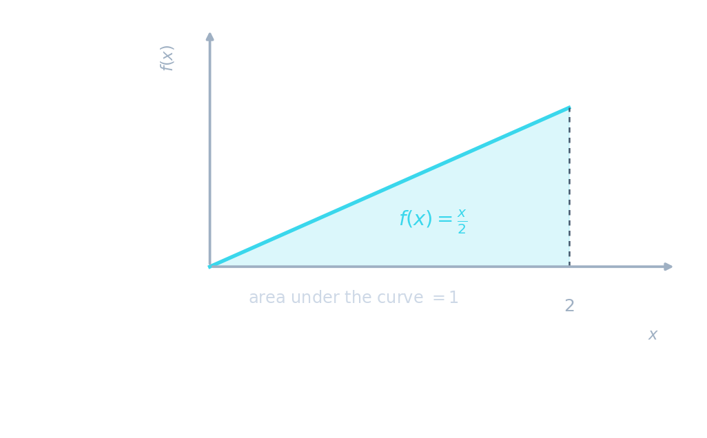
- For $f(x)=x/2$ on $0\leq x\leq2$, the total area is $\int_0^2x/2\,dx=1$. For example, $P(1<X<2)=\int_1^2x/2\,dx=3/4$.
- The probability $P(X=1)$ is $0$, although $f(1)=1/2$. A density height and a point probability are different quantities.
A variable has density f(x) = kx on [0,3], zero otherwise. Find k and P(1 < X < 2).
Compare the probability event, support, piecewise constants and calculation with the model. Revise the reasoning as well as the result.
Normalise a piecewise density
- A piecewise 分段 density can use different rules on different intervals. Suppose a graph is flat at height $a$ from $0$ to $2$, then falls linearly to zero at $4$. Its area is $2a+\tfrac12(2)a=1$, so $a=1/3$.
- The falling line has equation $(4-x)/6$. Thus our worked density is $f(x)=1/3$ for $0\leq x<2$, $f(x)=(4-x)/6$ for $2\leq x\leq4$, and $0$ otherwise. Normalisation 归一化 uses every piece, not a separate area of $1$ for each one.
Density area becomes cumulative height
$f(x)=2x/b^2,\quad F(x)=x^2/b^2\ (0\le x\le b)$
Match the rising density on [0, 2] to its cumulative probability. A bound selects an area; a percentile finds the bound for a given area.
A density is kx for 0 ≤ x < 1 and 2k for 1 ≤ x ≤ 2, zero otherwise. Find k. Must its two pieces meet at x = 1?
Compare the probability event, support, piecewise constants and calculation with the model. Revise the reasoning as well as the result.
Split an event at every density breakpoint
- For that worked density, $P(1<X<3)$ crosses $x=2$. Split the integral:
- The part from $2$ to $3$ has area $1/4$. Using the flat rule over the whole event would give the wrong probability.
A density is 2x/5 on [0,1) and 4/5 on [1,2], zero otherwise. Find P(1/2 < X < 3/2).
Compare the probability event, support, piecewise constants and calculation with the model. Revise the reasoning as well as the result.
A condition restricts and rescales the area
- Conditional probability 条件概率 uses $P(A\mid B)=P(A\cap B)/P(B)$ when $P(B)>0$. Translate the condition into a region before integrating.
- In the worked density, $P(X>3)=1/12$ and $P(X>1)=2/3$. Hence $P(X>3\mid X>1)=(1/12)/(2/3)=1/8$; the denominator is the allowed area after conditioning.
A density is 2x/5 on [0,1) and 4/5 on [1,2], zero otherwise. Find P(X > 3/2 given X > 1/2).
Compare the probability event, support, piecewise constants and calculation with the model. Revise the reasoning as well as the result.
Find expectation using density weights
- The expectation 期望, or mean, is $E(X)=\int x f(x)\,dx$ over the full support. The variable $x$ weights each small probability contribution.
- For the worked density,
A variable has density 3x² on [0,1], zero otherwise. Find its mean, showing the integrand.
Compare the probability event, support, piecewise constants and calculation with the model. Revise the reasoning as well as the result.
Calculate a second moment before variance
- The second moment is $E(X^2)=\int x^2 f(x)\,dx$. The variance 方差 is $\operatorname{Var}(X)=E(X^2)-[E(X)]^2$, not the integral of $x^2$ alone.
- The worked density gives $E(X^2)=10/3$, so $\operatorname{Var}(X)=10/3-(14/9)^2=74/81$. The mean lies inside the support and variance is nonnegative.
A variable has density 3x² on [0,1] and mean 3/4. Find its variance.
Compare the probability event, support, piecewise constants and calculation with the model. Revise the reasoning as well as the result.
Apply the general expectation rule
- For a function $g$, the syllabus rule is
provided the expectation exists. Substitute the requested function into the integrand; do not find a new density unless it is useful or requested.
- For $g(X)=3X+2$, $E(g(X))=3E(X)+2$. This linear shortcut does not extend to arbitrary functions: $E(X^2)$ is generally different from $[E(X)]^2$.
A variable has density 2x on [0,1], zero otherwise. Find E(3X² + 2) without deriving a transformed density.
Compare the probability event, support, piecewise constants and calculation with the model. Revise the reasoning as well as the result.
A reciprocal expectation needs its own integral
- For the original triangular density $f(x)=x/2$ on $[0,2]$,
- Here $E(X)=4/3$, so $1/E(X)=3/4$, a different answer. When an integrand has a singular endpoint, check that the improper integral is finite before reporting a mean; do not cancel an integration limit.
A variable has density 2x on (0,1). Find E(1/X) and compare it with 1/E(X).
Compare the probability event, support, piecewise constants and calculation with the model. Revise the reasoning as well as the result.
Define the cumulative function on the whole line
- The cumulative distribution function 累积分布函数 is $F(x)=P(X\leq x)=\int_{-\infty}^x f(t)\,dt$. It is nondecreasing, lies between $0$ and $1$, and is continuous for a distribution described by a density.
- Below the lowest possible value, $F=0$; above the highest possible value, $F=1$. The outside values belong to the CDF, even though the density is zero there.
The cumulative distribution function F(x) gives:
Difficulty 1/5 · 100 coins + a small bonus on first completion today
F(x) = P(X ≤ x), the accumulated area up to x.
A proposed CDF is 0 for x < −1, x² for −1 ≤ x ≤ 1, and 1 for x > 1. Explain why it cannot describe a variable with a density.
Compare the probability event, support, piecewise constants and calculation with the model. Revise the reasoning as well as the result.
Carry earlier probability into the next CDF piece
- In the worked density, $F(x)=x/3$ for $0\leq x<2$. For $2\leq x\leq4$, start with $F(2)=2/3$ and add only the new area:
- Complete the definition with $F=0$ for $x<0$ and $F=1$ for $x>4$. The two interior rules meet at $F(2)=2/3$; integrating the second density piece from zero would lose the accumulated constant.
A density is 2x/5 on [0,1) and 4/5 on [1,2], zero otherwise. Find its complete CDF.
Compare the probability event, support, piecewise constants and calculation with the model. Revise the reasoning as well as the result.
A density may jump while its CDF stays continuous
- Consider $f(x)=2x/7$ on $0\leq x<1$ and $f(x)=6/7$ on $1\leq x\leq2$, zero otherwise. Its total area is $1/7+6/7=1$; the density jumps at $1$.
- Its CDF is $x^2/7$ on $[0,1)$ and $(6x-5)/7$ on $[1,2]$. Both give $F(1)=1/7$. Their slopes differ: $F'=f$ inside each smooth piece, while the derivative at the join need not exist.
Inside a smooth piece, the probability density f(x) is the ______ of the cumulative function F(x).
Difficulty 1/5 · 100 coins + a small bonus on first completion today
Inside each smooth piece, f(x) = F′(x). At a density jump, the CDF stays continuous but its derivative may fail to exist.
For a density 2x/5 on [0,1) and 4/5 on [1,2], compare the one-sided density limits and CDF limits at x = 1. Does the CDF have a derivative there?
Compare the probability event, support, piecewise constants and calculation with the model. Revise the reasoning as well as the result.
Recover constants from a given CDF
- Suppose a continuous variable has $F=0$ below $1$, $F(x)=ax^2+b$ for $1\leq x\leq3$, and $F=1$ above $3$. Continuity gives $a+b=0$ and $9a+b=1$.
- Thus $a=1/8$, $b=-1/8$. Differentiating gives $f(x)=x/4$ on $1<x<3$, zero elsewhere. Check both endpoint values and nonnegative slope; two constants are not determined by the final endpoint alone.
A continuous variable has CDF 0 below 2, ax² + b on [2,4], and 1 above 4. Find a, b and its density.
Compare the probability event, support, piecewise constants and calculation with the model. Revise the reasoning as well as the result.
Use CDF differences for interval probabilities
- For a continuous distribution, $P(a<X\leq b)=F(b)-F(a)$; strict versus non-strict endpoints give the same result because point probabilities are zero.
- For the worked density, $F(3)-F(1)=11/12-1/3=7/12$, agreeing with the split integral. Either method must use the right CDF branch at each endpoint.
A variable has CDF (x² − 4)/12 on [2,4], with the usual outside values. Find P(5/2 ≤ X < 7/2), and explain whether changing either inequality to strict changes the result.
Compare the probability event, support, piecewise constants and calculation with the model. Revise the reasoning as well as the result.
Locate the median before solving
- The median 中位数 $m$ satisfies $F(m)=1/2$. In the worked density $F(2)=2/3$, so $m$ lies in the first piece: $m/3=1/2$, giving $m=3/2$.
- In the original triangular example, $F(x)=x^2/4$ on $[0,2]$, so $m=\sqrt2$. A density height $f(m)=1/2$ is not the median equation.
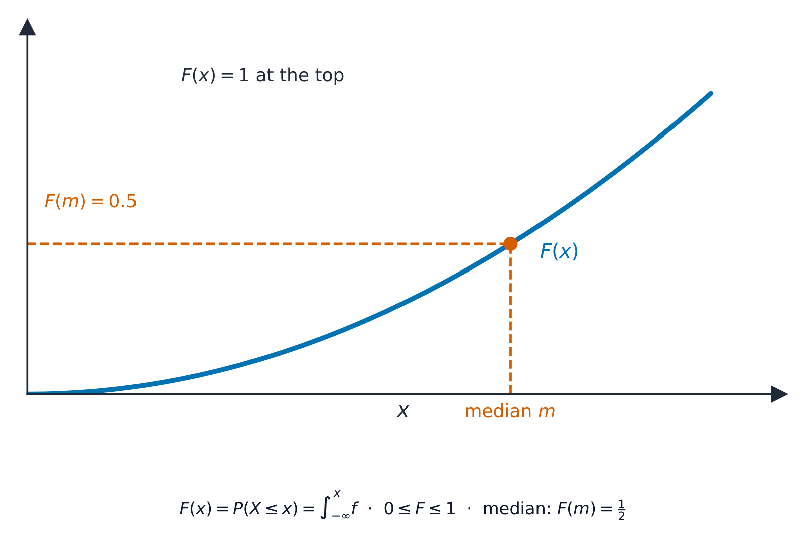
For f(x) = ½x on [0,2], F(x) = ¼x². The median solves ¼m² = 0.5. What is m? (2 dp)
Difficulty 2/5 · 140 coins + a small bonus on first completion today
¼m² = 0.5 → m² = 2 → m = √2 ≈ 1.41.
The median m of a continuous distribution satisfies:
Difficulty 1/5 · 100 coins + a small bonus on first completion today
The median splits the area in half: F(m) = 0.5.
A variable has density 3x² on [0,1], zero otherwise. Find its exact median and check its range.
Compare the probability event, support, piecewise constants and calculation with the model. Revise the reasoning as well as the result.
Choose the correct percentile branch
- A percentile 百分位数 at proportion $p$ solves $F(q)=p$. A lower quartile 四分位数 uses $p=1/4$. For the worked density, the lower quartile is $3/4$ because it lies below $2$.
- The 90th percentile lies above $2$: solve $1-(4-q)^2/12=0.9$. The valid root is $q=4-\sqrt{6/5}$; the other algebraic root lies outside the support. Check the branch after solving.
A continuous distribution is uniform from 2 to 6. What is the median, and why can a probability density be greater than 1?
For a uniform distribution the median and the mean are the centre of the interval. Probability is the area under the density.
A CDF is x²/5 for 0 ≤ x < 1, (4x − 3)/5 for 1 ≤ x ≤ 2, and 0 or 1 outside. Find the 10th and 90th percentiles.
Compare the probability event, support, piecewise constants and calculation with the model. Revise the reasoning as well as the result.
Start a transformation with an event and a range
- A transformation 变换 $Y=g(X)$ changes the range of possible values. First find the support of $Y$ and where each old breakpoint moves; then write $F_Y(y)=P(g(X)\leq y)$.
- Solve that event for $X$, use its CDF, and differentiate if a new density is required. Write $F_Y=0$ and $1$ outside its support, and $f_Y=0$ outside the density's support.
X can range over [−2,1] and Y = 2 − X². Find the full range of Y and explain why using only the endpoint images misses part of it.
Compare the probability event, support, piecewise constants and calculation with the model. Revise the reasoning as well as the result.
An increasing affine transformation preserves the event order
- For $Y=2X+1$ using the worked density, the support changes from $[0,4]$ to $[1,9]$ and the breakpoint $2$ becomes $5$. Since $2X+1\leq y$ means $X\leq(y-1)/2$,
- Differentiation gives $f_Y(y)=\tfrac12 f_X((y-1)/2)$: it is $1/6$ on $1<y<5$ and $(9-y)/24$ on $5<y<9$, zero otherwise. The inverse derivative supplies the factor $1/2$.
X has density 2x on [0,1], zero otherwise. Let Y = 3X + 2. Find the full CDF and density of Y.
Compare the probability event, support, piecewise constants and calculation with the model. Revise the reasoning as well as the result.
A decreasing transformation reverses the inequality
- Use the original triangular $X$ on $[0,2]$ and let $Y=4-X$, whose support is $[2,4]$. The event $4-X\leq y$ means $X\geq4-y$.
- Thus $F_Y(y)=1-F_X(4-y)=1-(4-y)^2/4$ for $2\leq y\leq4$, and $f_Y(y)=(4-y)/2$ inside that interval. Complete the outside pieces. Substituting into $F_X$ without the complement would produce a decreasing, invalid CDF.
X has density 2x on [0,1], zero otherwise. Let Y = 3 − 2X. Find the full CDF and density of Y.
Compare the probability event, support, piecewise constants and calculation with the model. Revise the reasoning as well as the result.
Keep the original positive-square transformation
- If the original triangular $X$ lies in $[0,2]$ and $Y=X^2$, the map is increasing on that support. For $0\leq y\leq4$,
- Hence $f_Y(y)=1/4$ on $(0,4)$ and zero otherwise: $Y$ is uniform on $[0,4]$. State the transformed support; the expression $y/4$ is not a CDF for every real $y$.
X is uniform on [1,2] and Y = X². Find the full CDF and density of Y.
Compare the probability event, support, piecewise constants and calculation with the model. Revise the reasoning as well as the result.
A cubic transformation can produce a tall density
- With the same triangular $X$, let $Y=X^3$. Its support is $[0,8]$, and $F_Y(y)=F_X(\sqrt[3]y)=y^{2/3}/4$ for $0\leq y\leq8$.
- For $0<y<8$, $f_Y(y)=1/(6y^{1/3})$. It becomes large near zero but has total area $1$. A density need not be bounded; values assigned at single endpoints do not change probabilities.
X is uniform on [0,2] and Y = X³. Find the full CDF and density of Y and check normalisation.
Compare the probability event, support, piecewise constants and calculation with the model. Revise the reasoning as well as the result.
Transform every branch for a cube root
- For $Y=\sqrt[3]X$ using the worked piecewise density, $X=y^3$. The support is $[0,\sqrt[3]4]$ and the old breakpoint $2$ becomes $\sqrt[3]2$.
- On the interior, $F_Y(y)=F_X(y^3)$ and $f_Y(y)=3y^2f_X(y^3)$. Thus the density is $y^2$ below $\sqrt[3]2$ and $y^2(4-y^3)/2$ above it, zero outside the new support. Keep the inverse's derivative factor.
X has density 3x² on [0,1], zero otherwise. For Y = cube root of X, find the full CDF and density.
Compare the probability event, support, piecewise constants and calculation with the model. Revise the reasoning as well as the result.
Use the same method for a square root
- For $Y=\sqrt X$ using the worked piecewise density, $X=y^2$, support is $[0,2]$ and the breakpoint is $\sqrt2$. For $y$ inside the support, $F_Y(y)=F_X(y^2)$.
- Differentiate: $f_Y(y)=2yf_X(y^2)$. This gives $2y/3$ for $0<y<\sqrt2$ and $y(4-y^2)/3$ for $\sqrt2<y<2$, zero otherwise. A formula with only the substitution misses the chain-rule multiplier.
X has density 3x² on [0,1], zero otherwise. Let Y = square root of X. Find the full CDF and density.
Compare the probability event, support, piecewise constants and calculation with the model. Revise the reasoning as well as the result.
A reciprocal needs a positive bounded support
- Let $X$ be uniform on $[1,3]$ and $Y=1/X$. The map is decreasing and the new support is $[1/3,1]$. Inside it, $Y\leq y$ means $X\geq1/y$.
- Hence $F_Y(y)=(3-1/y)/2$ and $f_Y(y)=1/(2y^2)$. The CDF is $0$ below $1/3$ and $1$ above $1$; the density is $0$ outside. The positive support makes the inequality reversal unambiguous.
X is uniform on [2,5] and Y = 1/X. Find the full CDF and density of Y.
Compare the probability event, support, piecewise constants and calculation with the model. Revise the reasoning as well as the result.
A square across zero can have two preimages
- Now let $X$ be uniform on $[-1,2]$ and $Y=X^2$. Then $Y\in[0,4]$, and $X^2\leq y$ means $-\sqrt y\leq X\leq\sqrt y$, intersected with $[-1,2]$.
- Thus $F_Y(y)=2\sqrt y/3$ for $0\leq y<1$, and $F_Y(y)=(1+\sqrt y)/3$ for $1\leq y\leq4$. Differentiate within each piece: the densities are $1/(3\sqrt y)$ and $1/(6\sqrt y)$. The negative preimage stops contributing once $\sqrt y>1$.
X is uniform on [−2,3] and Y = X². Find the complete piecewise CDF and density of Y.
Compare the probability event, support, piecewise constants and calculation with the model. Revise the reasoning as well as the result.
Absolute value also folds a range
- With $X$ uniform on $[-1,2]$ and $Y=|X|$, the support is $[0,2]$. The event is $-y\leq X\leq y$, clipped to the original support.
- Its CDF is $2y/3$ for $0\leq y<1$ and $(1+y)/3$ for $1\leq y\leq2$. The density is $2/3$ then $1/3$, zero outside. Two input values contribute before the shorter side ends; one contributes afterwards.
X is uniform on [−2,3] and Y = |X|. Find the full CDF and density of Y.
Compare the probability event, support, piecewise constants and calculation with the model. Revise the reasoning as well as the result.
Check a transformed probability two ways
- For $X$ uniform on $[-1,2]$ and $Y=X^2$, use the derived CDF:
- Directly, $1/2<|X|<3/2$ gives two intervals, $(-1,-1/2)$ and $(1/2,3/2)$, after clipping to the support. Their total length is $3/2$, divided by the original length $3$, again giving $1/2$.
X is uniform on [−2,3] and Y = X². Find P(1/4 < Y < 4) using both a transformed CDF and intervals for X.
Compare the probability event, support, piecewise constants and calculation with the model. Revise the reasoning as well as the result.
Find transformed moments without finding a new density
- For that same $X$ and $Y=X^2$, the general expectation rule gives $E(Y)=E(X^2)=1$ and $E(Y^2)=E(X^4)=11/5$.
- Therefore $\operatorname{Var}(Y)=11/5-1=6/5$. In contrast $[E(X)]^2=(1/2)^2=1/4$. Transforming the mean is generally different from taking the mean of a transformed variable.
X is uniform on [−2,3] and Y = X². Find E(Y) and Var(Y) without deriving the density of Y.
Compare the probability event, support, piecewise constants and calculation with the model. Revise the reasoning as well as the result.
Audit the distribution before accepting an answer
- A density must be nonnegative and integrate to $1$ across all its pieces. Its CDF must be continuous, nondecreasing, have correct outside values, and differentiate to the density inside each smooth piece.
- For a transformed variable, check support, moved breakpoints, all valid inverse branches and the derivative multiplier. Use an independent event probability or moment as a second check; reject a root outside its branch even if its algebra is correct.
X is uniform on [1,2] and Y = 1/X. A proposed interior CDF is F_X(1/y) = 1/y − 1 on [1/2,1]. Diagnose the error and give the correct full CDF and density.
Compare the probability event, support, piecewise constants and calculation with the model. Revise the reasoning as well as the result.
Retrieve the area and event methods
- Probability is density area; expectation is a weighted integral; a percentile solves a CDF equation on a checked branch. A piecewise CDF must include earlier accumulated area.
- For $Y=g(X)$, start with $P(g(X)\leq y)$ and the new support. Increasing, decreasing and folded transformations lead to different events; differentiate only after getting that event right.
A continuous distribution is uniform from 2 to 6. What is its median?
Difficulty 1/5 · 100 coins + a small bonus on first completion today
The midpoint of 2 and 6 is 4. Other options — 1 (the total area under a density); 1.41 (the lesson median).