What this course is, and how to use it
This is the fifth course in University Mechanical Engineering: thermodynamics 热力学 — energy, entropy and the machinery that turns one into work: how to account for it, how far it can go, and how to know a claim about a machine is impossible before building it.
Scope limit, stated once: a study course, not a degree; the teaching fluids are water, air and R-134a, every cycle is checked by both laws in the course suite, and every table value used here is recomputed there from the quoted source constants.
- Units 5.1–5.3 build the accounting: state, closed systems, open systems.
- Unit 5.4 sets the limits: the second law and entropy.
- Units 5.5–5.6 spend the limits: power cycles and refrigeration.
The thermo habit: every cycle is checked by both laws — the suite runs the checks; the habit is looking before believing.
Properties and state
Why it matters. Before any law can be applied, the working fluid must be pinned down: what its state 状态 is, and which numbers move together.
The idea, with a picture. A state is a point on a property diagram 状态图; two independent intensive properties fix it. On the saturation dome 饱和线 the two-phase region sits under the dome; quality 干度 $x$ = vapour mass fraction walks across it.
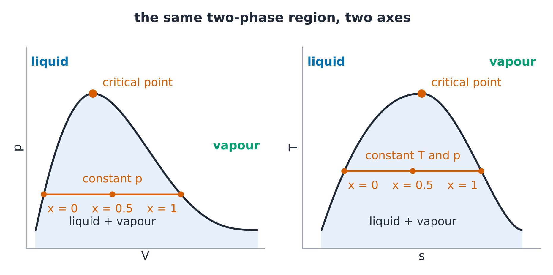
The derivation (why two properties fix the rest). A simple compressible substance obeys a two-variable equation of state, $p = p(v, T)$, so any other equilibrium property is a function of the same pair — pick two independent ones (inside the dome, $x$ is the walker) and everything else is determined.
Worked example 1 — reading a table row. Saturated water at $T = 100\,{}^\circ\mathrm{C}$: $p_{sat} = 101.35\ \mathrm{kPa}$, $v_f = 0.001044\ \mathrm{m^3/kg}$, $v_g = 1.6729\ \mathrm{m^3/kg}$, $h_f = 419.04\ \mathrm{kJ/kg}$, $h_{fg} = 2257.0\ \mathrm{kJ/kg}$. At $x = 0.5$: $v = v_f + x(v_g - v_f) = 0.837\ \mathrm{m^3/kg}$, $h = h_f + x\,h_{fg} = 1547.5\ \mathrm{kJ/kg}$ — the linear-in-$x$ rule holds for $v$, $u$, $h$, $s$ because dome properties differ only by the latent term.
Worked example 2 — ideal-gas territory. Air at $300\ \mathrm{K}$, $101.325\ \mathrm{kPa}$: $pv = RT$ with $R = 0.287\ \mathrm{kJ/(kg \, K)}$ gives $v = RT/p = 0.8497\ \mathrm{m^3/kg}$. At $2\times$ that pressure, same $T$: $v = 0.4248\ \mathrm{m^3/kg}$ — exactly half: the isotherm is a hyperbola (suite-checked both ways).
Common mistakes. Using $v$ averaged by volume instead of mass (quality is a mass fraction). Reading a superheated row from a saturation column. Treating $pv = RT$ inside the dome (ideal gas ends where condensation begins).
Summary. Two independent properties fix the state; the dome needs $x$ as the walker; linear-in-$x$ between $f$ and $g$; $pv = RT$ only outside the dome.
First law for closed systems
Why it matters. The first law is the accountant: energy changes by work and heat crossing the boundary, nothing else, and a closed system is the simplest ledger to keep.
The idea, with a picture. $\Delta E = Q - W$ (work by the system positive). On a p–V diagram the boundary work 边界功 $W = \int p\, dV$ is the area under the path — so the work depends on the path, not just the endpoints.
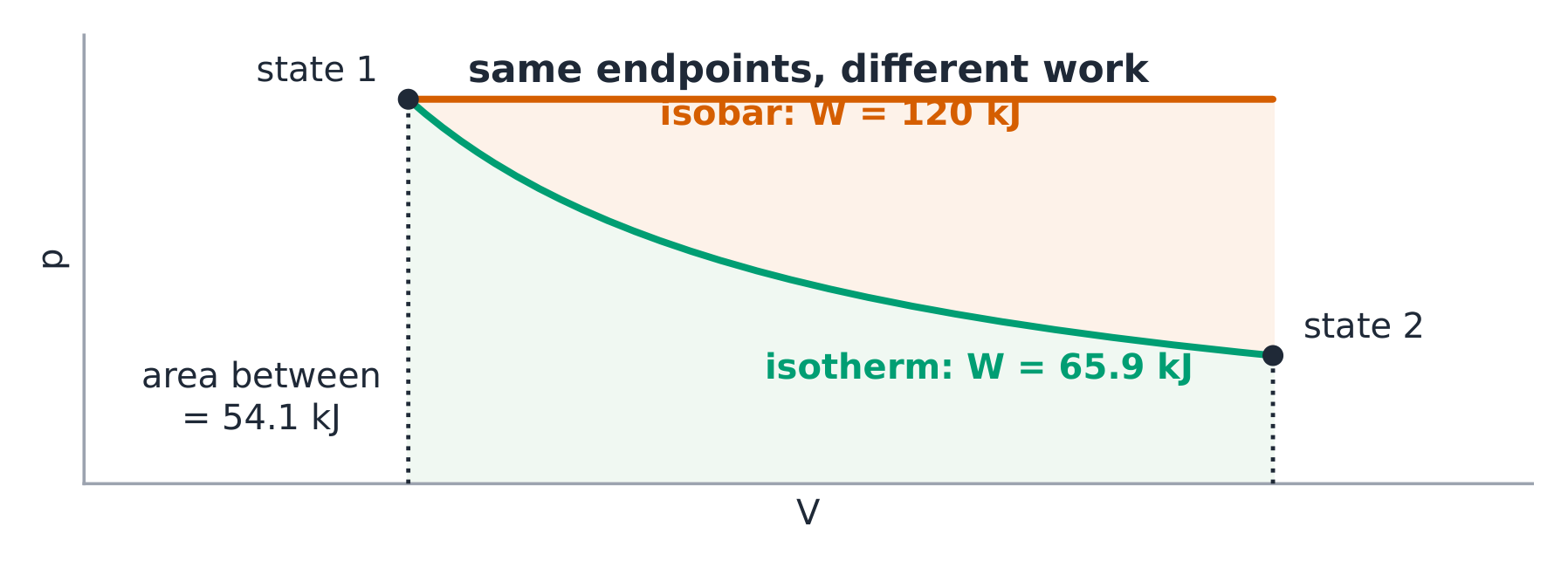
The derivation (why work is path-dependent). $W = \int_1^2 p\,dV$ integrates the path $p(V)$ itself, and different connective paths trace different curves between the same endpoints — only $U$ (and $H$, $S$) are state functions, the whole reason a cycle's net $\oint \delta W = \oint \delta Q$ closes.
Worked example 1 — three paths, one pair of states. Air from $(200\ \mathrm{kPa}, 0.3\ \mathrm{m^3})$ to $(200\ \mathrm{kPa}, 0.9\ \mathrm{m^3})$ versus via an isotherm through the same ends. At constant $p$: $W = p \Delta V = 200 \times 0.6 = 120\ \mathrm{kJ}$. Isothermal from $v_1 = v$ to $3v$: $W = mRT\ln(v_2/v_1) = p_1 V_1 \ln 3 = 200 \times 0.3 \times 1.0986 = 65.9\ \mathrm{kJ}$ — same endpoints, $54\ \mathrm{kJ}$ apart, the area between the curves is exactly the difference (suite-asserted).
Worked example 2 — the adiabatic check. Same start, compressed adiabatically ($Q = 0$) to $0.15\ \mathrm{m^3}$: $pV^\gamma = \mathrm{const}$ with $\gamma = 1.4$ gives $p_2 = 200 \times (0.3/0.15)^{1.4} = 527.8\ \mathrm{kPa}$; $W = (p_2 V_2 - p_1 V_1)/ (1 - \gamma) = (79.2 - 60)/(1 - 1.4) = 48\ \mathrm{kJ}$ of work on the gas; $\Delta U = -W = +48\ \mathrm{kJ}$ — the ledger closes.
Common mistakes. Sign errors on $W$ (by vs on). Using $p_1 V_1 \approx mRT$ with $V$ in litres and $R$ in $\mathrm{kJ}$. Forgetting that $\Delta U = m c_v \Delta T$ holds for ideal gas even when the process is not constant-volume — it is a property relation.
Summary. $\Delta U = Q - W$; boundary work is area under the path; state functions versus path functions; the ideal-gas toolkit ($pv = RT$, $c_v$, $c_p$, $pV^\gamma$ for reversible adiabatic).
First law for open systems
Why it matters. Real machines are pipes, not pistons: mass flows through a control volume 控制体积 and carries energy with it, and steady-state analysis is where turbines, pumps and nozzles live.
The idea, with a picture. The steady-flow energy equation per inlet/outlet port: $q - w = \Delta h + \Delta ke + \Delta pe$. The flow work $pv$ hides inside $h = u + pv$.
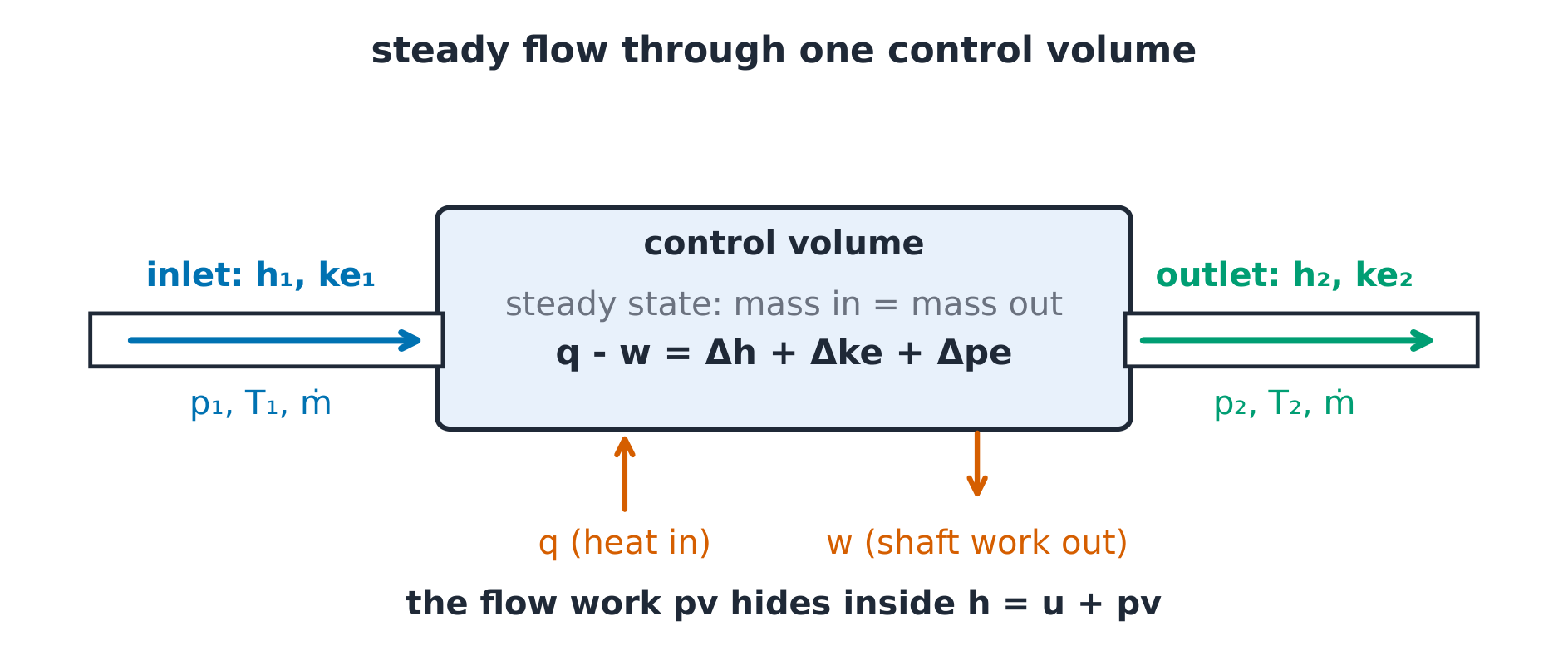
The derivation (where $pv$ goes). Pushing 1 kg of fluid into the control volume costs $p v$ (pressure times volume) of flow work; the same term reappears pushing it out. Combining that transport term with internal energy gives enthalpy — which is why the open-system ledger runs on $h$, not $u$: the bookkeeping absorbed the flow work.
Worked example 1 — a turbine stage. Steam enters at $3\ \mathrm{MPa}$, $400\,{}^\circ\mathrm{C}$ ($h_1 = 3230.9\ \mathrm{kJ/kg}$, $s_1 = 6.9212\ \mathrm{kJ/(kg\,K)}$) and expands adiabatically to $50\ \mathrm{kPa}$. Ideal (isentropic 等熵): $s_2 = s_1$ gives $x_2 = (6.9212 - 1.0910)/6.5029 = 0.89655$, so $h_{2s} = h_f + x\,h_{fg} = 340.49 + 0.89655 \times 2305.4 = 2407.4\ \mathrm{kJ/kg}$; $w_s = h_1 - h_{2s} = 823.5\ \mathrm{kJ/kg}$. With $\eta_t = 0.85$: $w = 0.85 \times 823.5 = 700.0\ \mathrm{kJ/kg}$, $h_2 = 3230.9 - 700.0 = 2530.9$ — the suite recomputes both legs.
Worked example 2 — a pump and a nozzle. Pump lifts liquid water $0.5\ \mathrm{MPa} \to 3\ \mathrm{MPa}$: $w_p \approx v\,\Delta p = 0.001005 \times 2500 = 2.5\ \mathrm{kJ/kg}$. Nozzle accelerates air $10 \to 300\ \mathrm{m/s}$ adiabatically, no work: $\Delta h = -\Delta ke = -(300^2 - 10^2)/2 = -44.95\ \mathrm{kJ/kg}$, $h_2 = h_1 - 44.95$. Three devices, one equation, the ports carry the ledger.
Common mistakes. Dropping $ke$ for a nozzle (it is the point of the device) or keeping it for a pump (negligible there). Using $c_p \Delta T$ for the exit of a two-phase expansion (inside the dome $h$ is not $c_p \Delta T$ from a superheated start). Forgetting $\dot W = \dot m\, w$ for the power answer.
Summary. $q - w = \Delta h + \Delta ke + \Delta pe$; enthalpy absorbs the flow work; $ke$ matters where velocity is the product; isentropic then efficiency is the two-step turbine method.
Second law and entropy
Why it matters. The first law only balances; the second law forbids. Entropy is the accounting quantity of the forbidden, and the Carnot bound stops bad machine claims on paper.
The idea, with a picture. $ds = \delta q_{rev}/T$ — entropy 熵; $\sigma \ge 0$ for every process, $= 0$ only for reversible ones. On a T–s diagram T–s 图 the reversible heat is area under the curve, and the $\eta_C = 1 - T_L/T_H$ appears as the rectangle ratio.
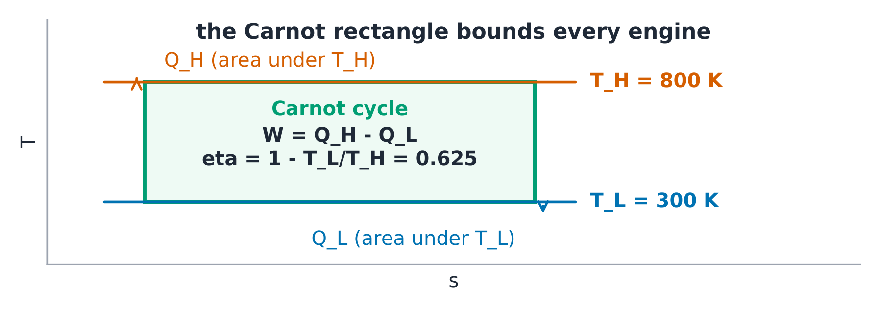
The derivation (Kelvin–Planck to Carnot). No cycle converts heat from one reservoir fully into work; so for a reservoir pair the best cycle must reject the least, and a reversible one must be the best (otherwise running it backwards would break the law). The reversible pair of isotherms and adiabats — Carnot — then has $Q_H/T_H = Q_L/T_L$ exactly, giving $\eta_C = 1 - T_L/T_H$. Between $800\ \mathrm{K}$ and $300\ \mathrm{K}$: $\eta_C = 0.625$; a claimed 0.70 engine between them is impossible, no prototype needed.
Worked example 1 — entropy balance on an irreversible adiabatic valve. Steam at $1000\ \mathrm{kPa}$, $h = 3059\ \mathrm{kJ/kg}$, $s = 7.155\ \mathrm{kJ/(kg\,K)}$ throttled to $200\ \mathrm{kPa}$ ($h_2 = h_1$): at $200\ \mathrm{kPa}$, $h = 3059$ is superheated, $s_2 = 7.289\ \mathrm{kJ/(kg\,K)}$; $\sigma = s_2 - s_1 = 0.134\ \mathrm{kJ/(kg\,K)} > 0$ — irreversible with no heat transfer at all.
Worked example 2 — the Carnot ledger. A Carnot engine takes $1000\ \mathrm{kJ}$ from $800\ \mathrm{K}$, rejects to $300\ \mathrm{K}$: $W = 625\ \mathrm{kJ}$, $Q_L = 375\ \mathrm{kJ}$, $\Delta S_{hot} = -1.250$, $\Delta S_{cold} = +1.250$: universe unchanged — reversible. Burn the same fuel irreversibly at $2000\ \mathrm{K}$ before transferring: $\sigma = Q(1/800 - 1/2000) = 0.75\ \mathrm{kJ/K}$ — the lost work $T_0 \sigma = 300 \times 0.75 = 225\ \mathrm{kJ}$, exactly the exergy destroyed.
Common mistakes. $ds = \delta q/T$ applied to an irreversible path (it needs $q_{rev}$, or use the entropy balance with $\sigma$). Reading efficiency claims without the reservoir temperatures. Taking $s$ constant across a throttling (throttle keeps $h$, not $s$).
Summary. $ds = \delta q_{rev}/T$; $\sigma \ge 0$; Carnot bounds by reservoir ratio; lost work $= T_0 \sigma$; T–s area = reversible heat.
Power cycles
Why it matters. The power plant is where the two laws pay rent: the Rankine cycle converts fuel to shaft work through phase change, and its efficiency is a battlefield of boiling pressure, superheat and reheat.
The idea, with a picture. The basic Rankine cycle 朗肯循环: pump $\to$ boiler $\to$ turbine $\to$ condenser, drawn on both p–V and T–s. Heat in at the high-pressure isobar, work out at the isentropic expansion, heat out at the condenser, work in at the pump.
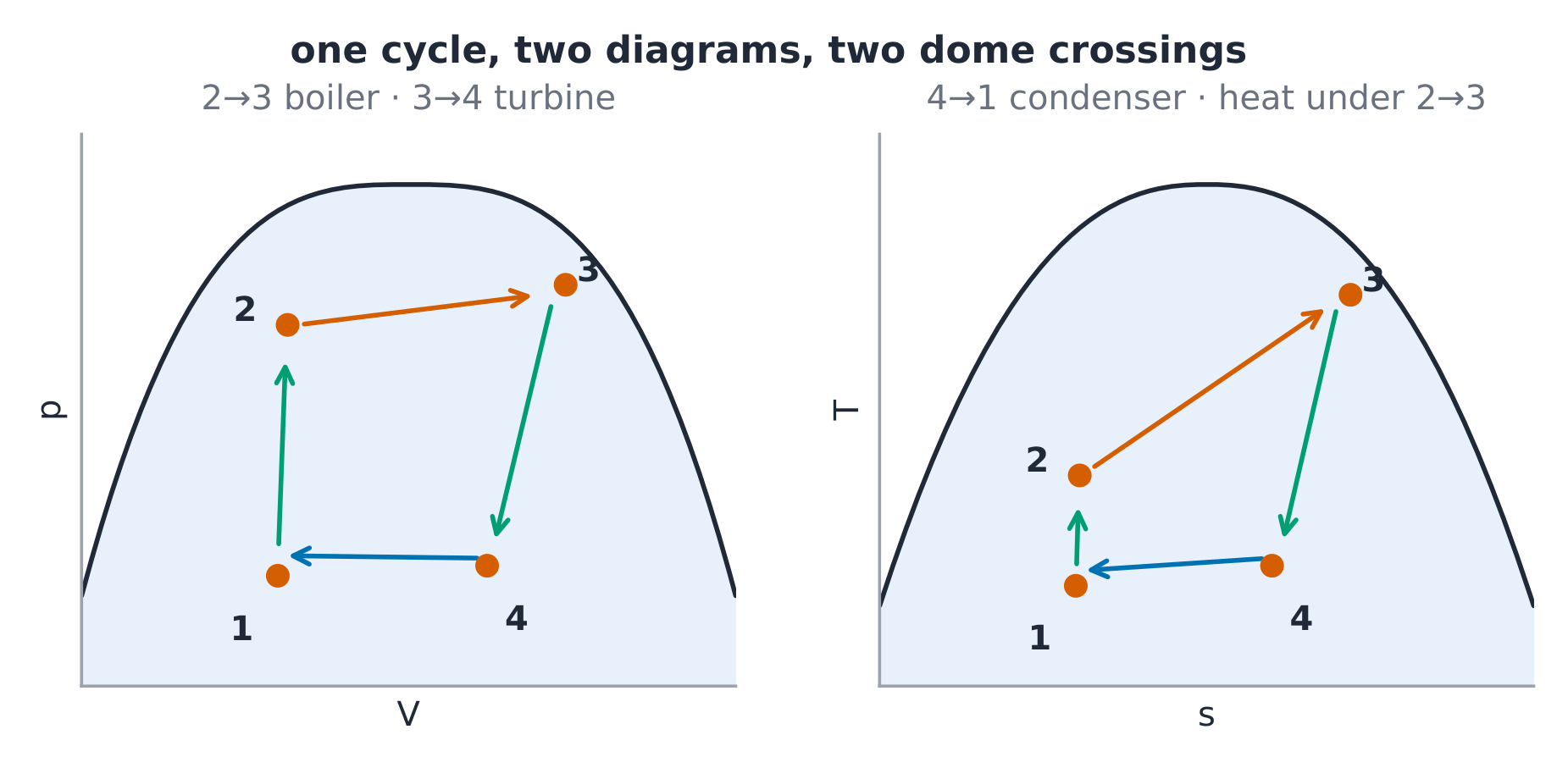
The derivation (why the boiler pressure raises efficiency). The cycle heat-in average temperature rises with boiler pressure, and the second-law ceiling $\eta \le 1 - T_{out}/T_{in,avg}$ rises with it. Meanwhile the pump work grows only as $v \Delta p$ (liquid $v$ is tiny), so the gain outruns the cost until metallurgy stops it. The suite demonstrates: the same cycle at $1\ \mathrm{MPa}$ versus $4\ \mathrm{MPa}$ moves $\eta$ from $25.3\%$ to $32.3\%$ with the same $T_{max}$.
Worked example 1 — the ideal Rankine baseline. Boiler at $4\ \mathrm{MPa}$, saturated vapour ($h_3 = 2801.4\ \mathrm{kJ/kg}$, $s_3 = 6.0700$); condenser at $10\ \mathrm{kPa}$. Turbine: $s_4 = s_3$ gives $x_4 = (6.0700 - 0.6492)/7.5009 = 0.7227$, $h_4 = 191.81 + 0.7227 \times 2392.8 = 1921.1$. Pump: $h_2 = h_1 + v_f (p_2 - p_1) = 191.81 + 0.001010 \times 3990 = 195.8$. Work out $2801.4 - 1921.1 = 880.3$, work in $4.0$; heat in $2801.4 - 195.8 = 2605.6$; $\eta = 876.3/2605.6 = 33.6\%$ — every step suite-verified.
Worked example 2 — two upgrades, priced. Superheat to $4\ \mathrm{MPa}$, $480\,{}^\circ\mathrm{C}$ ($h_3 = 3398.3$, $s_3 = 6.7677$): $x_4 = 0.8157$, $h_4 = 2143.6$; $\eta$ rises to $39.1\%$, and the exhaust quality climbs from 0.72 toward 0.82 — better, though still wet: real plant runs superheat and reheat to stay dry. Reheat from an intermediate $800\ \mathrm{kPa}$ back to $480\,{}^\circ\mathrm{C}$ pushes the exhaust above 0.9, clearing the 0.88 blade-erosion line.
Common mistakes. Subtracting $h_1$ instead of $h_2$ in the heat-in term (the pump outlet is where heat starts). Setting $s_2 = s_1$ across the pump (it nearly is, but use $h_2 = h_1 + v\Delta p$). Ignoring exhaust quality — a fine cycle can still ruin blades.
Summary. Four components, two dome crossings; isentropic turbine, liquid pump; superheat and reheat buy efficiency and dry exhaust; boiler pressure raises $T_{avg}$ in.
Refrigeration and heat pumps
Why it matters. Running the cycle backwards moves heat uphill — one skeleton serves the refrigerator and the heat pump alike.
The idea, with a picture. The vapor-compression cycle 蒸气压缩循环: compressor $\to$ condenser $\to$ throttle $\to$ evaporator. Performance is $\mathrm{COP}_R = q_L/w_{in}$ or $\mathrm{COP}_{HP} = q_H/w_{in}$. The reversed-Carnot 卡诺 bounds are $\mathrm{COP}_R \le T_{cold}/(T_{hot}-T_{cold})$ for cooling and $\mathrm{COP}_{HP} \le T_{hot}/(T_{hot}-T_{cold})$ for heating. Use absolute temperatures in kelvin.
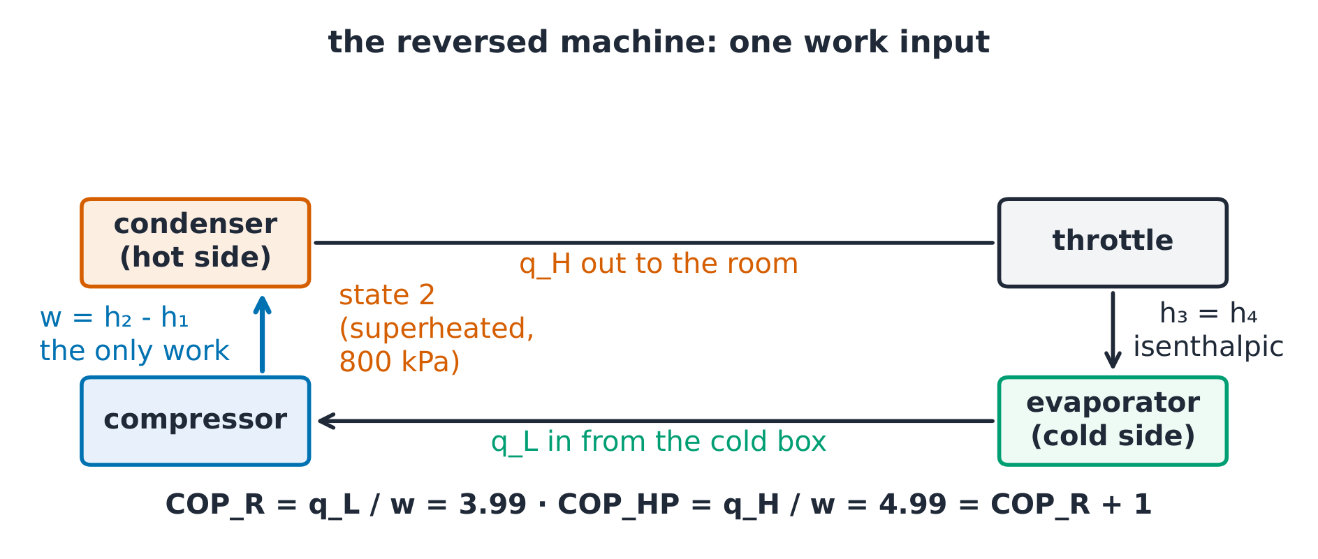
The derivation (why the throttle, not a turbine). The expansion could recover work — but the flow is wet and two-phase turbines are not worth it; a throttle is cheap, isenthalpic, destroys only a few kJ/kg, and the compressor simply re-pays them.
Worked example 1 — an R-134a refrigerator. Evaporator $-10\,{}^\circ\mathrm{C}$ ($h_1 = 394.6\ \mathrm{kJ/kg}$, $s_1 = 1.729\ \mathrm{kJ/(kg\,K)}$); compressor to $800\ \mathrm{kPa}$ isentropically: $h_2 = 432.9$ (superheated). Condenser exit saturated liquid $h_3 = 241.8$; throttle keeps $h_4 = 241.8$. Then $q_L = h_1 - h_4 = 152.8$, $w_{in} = 38.3$, $\mathrm{COP}_R = 152.8/38.3 = 3.99$. Reversed-Carnot between $-10$ and $31.3\,{}^\circ\mathrm{C}$: bound = $263.2/(304.5 - 263.2) = 6.37$ — real COP sits below, as it must.
Worked example 2 — the same machine heating. As a heat pump, $q_H = h_2 - h_3 = 432.9 - 241.8 = 191.1$ and $\mathrm{COP}_{HP} = 191.1/38.3 = 4.99 = \mathrm{COP}_R + 1$ ✓ — the same numbers read at different ports (suite-asserted).
Common mistakes. $\mathrm{COP} = w/q$ (inverted — COP is benefit over cost). Applying the reversed-Carnot bound with temperature differences instead of absolute temperatures. Reading $h_2$ from the saturated-vapour row (the exit is superheated).
Summary. Reverse the skeleton, swap turbine for throttle; the compressor is the only work; COP is benefit over cost under the reversed-Carnot ceiling, with $\mathrm{COP}_{HP} = \mathrm{COP}_R + 1$.