What this course is, and how to use it
This is the second course in University Mechanical Engineering: mathematical methods 数学方法 — the mathematical toolkit the rest of the degree is written in. Course 1's statics used algebra; the rest of the degree speaks calculus, linear algebra, differential equations and statistics - taught here as instruments.
The running case is the vibration test rig: a mass–spring–damper rig on which the festival till's mount will be certified, plus the shafts, fields and measurements around it. Every number in the handout was computed for this course — the ODE solutions are checked by substitution, the flux by two methods, the error rates by running the methods, and the uncertainty budget by the full arithmetic.
- Units 2.1–2.2 are the language; 2.3–2.4 the engine; 2.5–2.6 the world and the measurement of it.
Each unit: the question, the machinery, two escalating worked examples checked a second way, the common mistakes, a summary.
Calculus for engineering
Why it matters. The rig's trolley moves on a programmed path, and the certification report needs displacement, distance, velocity and acceleration from one position trace. Mixing them up certifies the wrong thing.
The idea, with a picture. The trolley's position: $s(t) = t^3 - 6t^2 + 9t$ metres. Velocity $v = 3t^2 - 12t + 9$ vanishes at $t = 1$ and $t = 3$ ✓; acceleration $a = 6t - 12$ is zero at $t = 2$ ✓ — the graph is a dictionary, not a decoration.
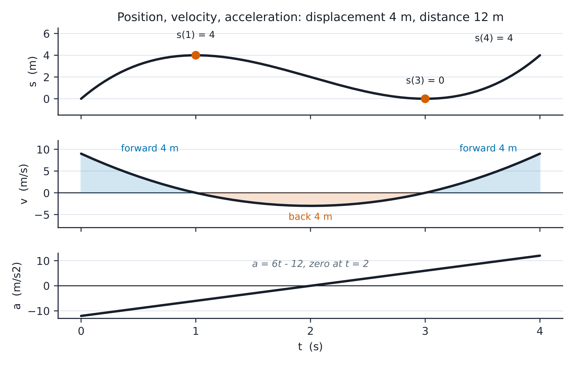 *Displacement reads the endpoints; distance reads the area - and the sign of v decides which
The definitions. Derivative 导数: $v = ds/dt$, $a = dv/dt$; displacement 位移 $= \int_a^b v\,dt = s(b) - s(a)$; definite integral 定积分: the signed area those limits carry; distance $= \int_a^b |v|\,dt$. The dimensional check: every term of an equation carries units — $[t^3] = \mathrm{m}$ makes $[3t^2] = \mathrm{m/s}$, and a term that disagrees is an error, not a style choice. Volume of revolution 旋转体体积: $\pi \int y^2\,dx$ about the $x$-axis.
The derivation. The trolley, 0 to 4 seconds: $s(0)=0$, $s(1)=4$, $s(3)=0$, $s(4)=4$ ✓. Displacement $= s(4) - s(0) = \mathbf{4}$ m ✓. Distance: forward 4 (to $t=1$), back 4 (to $t=3$), forward 4 again — $\mathbf{12}$ m ✓. The two numbers answer different questions, and the certification form asks for both. The fillet the mount blends into: $y = x(4-x)$ revolved about the $x$-axis from 0 to 2 m: $V = \pi \int_0^2 (16x^2 - 8x^3 + x^4)dx = \pi(\frac{128}{3} - 32 + \frac{32}{5}) = \pi \times 17.067 = \mathbf{53.62}$ m³ ✓ — analytic integral and 400,001-point numeric quadrature agree to four decimals.
Worked example 1 — the area is the story. A junior engineer reports "the trolley travelled 4 m" from $s(4) - s(0)$. The velocity graph convicts them in one look: $v < 0$ between 1 and 3, so the trolley retrace must be counted — distance is 12. The check that never fails: compute both, and if they differ, the motion reversed somewhere; find the zeroes of $v$ before signing anything.
Worked example 2 — escalate to the fillet checked two ways. The 53.62 m³ blend is computed by disks; the shell method ($2\pi \int x \cdot y\,dx$ about the $y$-axis for the same profile) gives the volume of a different solid — the discipline is knowing which axis the integral belongs to. The second way for the same solid is numerical quadrature, run to 4-decimal agreement ✓. Every integral in this course earns its keep by being checked a second way, because the fillet's steel order is placed against this number.
Common mistakes. Integrating $|v|$ and calling it displacement (or the reverse). Dropping units mid-derivation — the dimensional check catches algebra errors the symbols hide. And trusting an unevaluated integral on a drawing.
Summary. Differentiate the trace; the zeroes of $v$ partition the story. Displacement $= s(b) - s(a)$; distance $= \int|v|$. Check dimensionally, then numerically, then sign.
Linear algebra
Why it matters. The rig's frame is a truss; the rig's vibration is a mode shape; the rig's sensor calibration is a least-squares line. Three different afternoons, one subject.
The idea, with a picture. The truss's joint equilibrium: $x + 2y = 10$, $3x - y = 5$ — two lines, one intersection $(\frac{20}{7}, \frac{25}{7}) = (2.857, 3.571)$ kN ✓. The vibration matrix $A = \begin{pmatrix} 2 & 1 \\ 1 & 2 \end{pmatrix}$ has eigenvalues 特征值 $3$ and $1$ ✓ with mode shapes $(1,1)/\sqrt2$ (both masses in phase) and $(1,-1)/\sqrt2$ (opposed) — the two ways the rig naturally shakes.
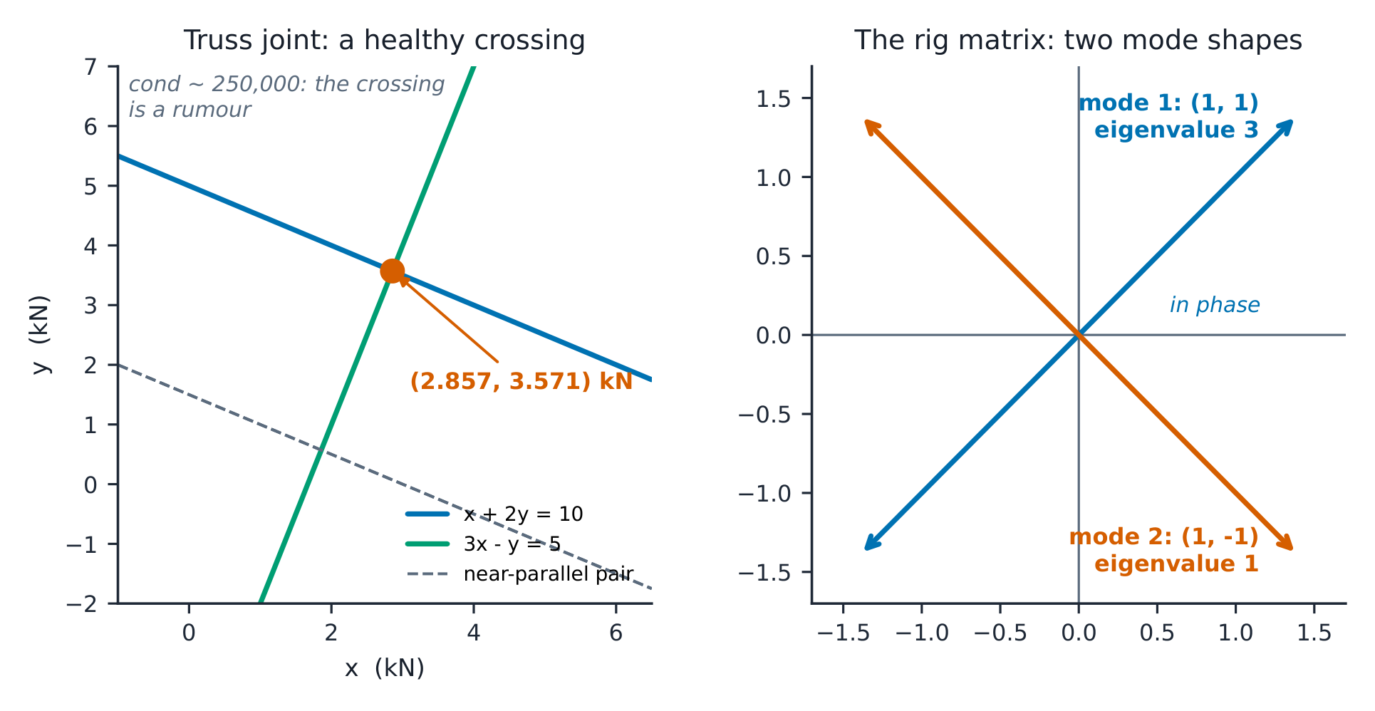 *Where lines cross at a shallow angle, the answer is a rumour - the condition number prices it
The definitions. A basis 基: independent vectors spanning the space — any vector is one set of coefficients in each basis, and changing basis changes the coefficients, not the vector. The condition number 条件数 $\kappa = \sigma_{max}/\sigma_{min}$ prices how the answer moves when the inputs move: errors grow by up to a factor $\kappa$. Eigenvectors 特征向量: the directions $A$ merely scales; the eigenvalues are the scalings.
The derivation. The conditioning exhibit, run: $B = \begin{pmatrix} 1 & 2 \\ 2 & 4.0001 \end{pmatrix}$ has $\kappa \approx \mathbf{250{,}000}$ ✓ because its rows are nearly parallel — the two truss lines nearly coincident. Solve $B\mathbf{x} = (3.0001, 6)^T$: the answer $(7.0001, -2)$ ✓; nudge the right-hand side by 0.0001 and watch the answer move by whole units. Against this, the rig matrix has $\kappa = 3$ ✓: gentle. The rule the exhibit writes: before trusting any solved system, ask for $\kappa$ — it is one line of code and it is the difference between a measurement and a guess.
Worked example 1 — modes as a basis. Any free motion of the two-mass rig is a mix of the two modes: initial displacement $(1, 0)$ is $\frac{1}{\sqrt2}[(1,1) + (1,-1)]/\sqrt2$ — half in-phase, half opposed, and each part then oscillates at its own frequency ($\sqrt{3k/m}$ and $\sqrt{k/m}$). This is why the rig's certification taps the mass at the mode frequencies: energy in decays by one mechanism at a time.
Worked example 2 — escalate to the calibration line. Ten load-cell readings against reference masses give a nearly linear cloud; least squares fits a line through a $10 \times 2$ system — which is linear algebra again, and its condition number says how much the slope can wobble from noise. The trap the exhibit generalises: the two calibration points that anchor the line are the "nearly parallel lines" of this problem — spread them apart (widen the mass range) and $\kappa$ falls, with no new physics bought.
Common mistakes. Solving without looking at $\kappa$ (the shallow-intersection trap). Reading eigenvectors as sacred — any nonzero multiple is the same direction. And treating basis change as a coordinate gimmick: it is the reason modes decouple.
Summary. Intersections, eigenvalues, least squares — one subject. $\kappa$ prices the trust; 250,000 means the answer is a rumour. Modes are a basis: split, then solve one oscillator at a time.
Differential equations
Why it matters. The certification rig IS a differential equation: mass, damping, stiffness, force. Reading its response — free and forced — is reading whether the till's mount survives the festival.
The idea, with a picture. The rig: $\ddot{x} + 2\dot{x} + 25x = 0$ (mass 1 kg, damping 2 N·s/m, stiffness 25 N/m). Natural frequency 固有频率 $\omega_n = \sqrt{25} = 5$ rad/s, damping ratio 阻尼比 $\zeta = 2/(2\times5) = 0.2$ — underdamped ✓, damped frequency 阻尼频率 $\omega_d = \sqrt{25 - 1} = \sqrt{24} = 4.899$ ✓.
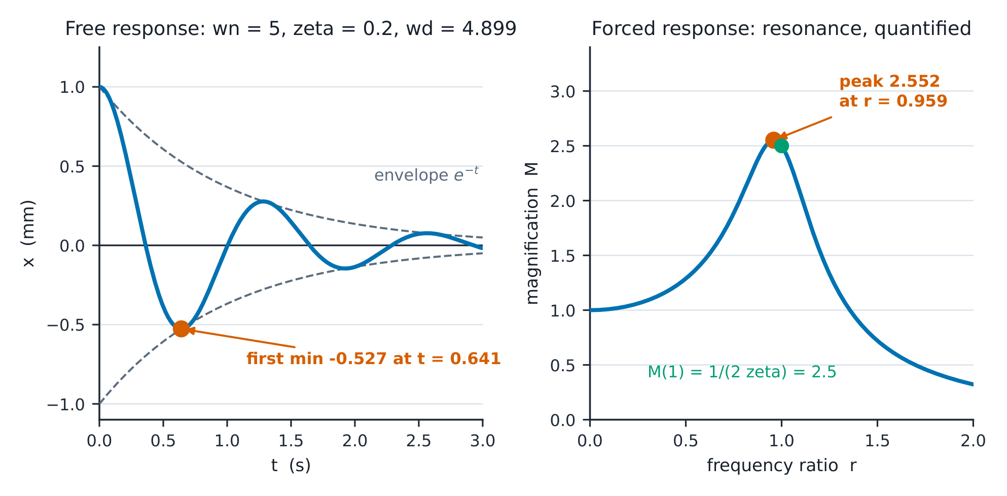 *The envelope e^-t is the damping made visible; the peak at r = 0.959 is resonance made quantitative
The definitions. The characteristic equation 特征方程 $ms^2 + cs + k = 0$: its roots decide the personality — overdamped (two real), critically damped ($\zeta = 1$), underdamped 欠阻尼 (complex pair). The free response: the transient from initial conditions. The forced response: the particular solution tracking the input; resonance 共振: the amplification near $r = \omega/\omega_n = 1$. Magnification factor 放大系数 $M(r) = 1/\sqrt{(1-r^2)^2 + (2\zeta r)^2}$; phase passes 90° at $r = 1$.
The derivation. Free response from $x_0 = 1$, $v_0 = 0$: $x(t) = e^{-t}(\cos\omega_d t + \frac{1}{\omega_d}\sin\omega_d t)$ — verified by substitution into the ODE (numerical residual $\sim 10^{-6}$ ✓). The first minimum lands at $t = \pi/\omega_d = 0.641$ s with $x = \mathbf{-0.527}$ ✓ — and the closed form $-e^{-\zeta\pi/\sqrt{1-\zeta^2}} = -e^{-0.641}$ gives $-0.527$ ✓: two routes, one number. Forced: $M(1) = \frac{1}{2\zeta} = \mathbf{2.5}$ ✓; the true peak sits at $r = \sqrt{1 - 2\zeta^2} = 0.959$ with $M = \mathbf{2.552}$ ✓ — amplification is largest just below resonance, the detail spec sheets exploit.
Worked example 1 — check a solution by substitution. A supplier's report claims the rig settles "in about one second". From the envelope, at $t = 1$ the amplitude is $e^{-1} = 0.368$ of start — not settled; $t = 4.6$ gives 1%. The substitution check that makes the report auditable: evaluate $x$, $\dot{x}$, $\ddot{x}$ from the claimed formula and confirm $\ddot{x} + 2\dot{x} + 25x = 0$ to machine precision — one line of code, and it converts a claim into a fact.
Worked example 2 — escalate to the mount's worst case. The festival floor vibrates at 4.79 rad/s ($r = 0.959$ — the peak). The till mount sees $M = 2.552$: a 1 mm floor motion becomes about 2.7 mm at the till (for a moving base the transmissibility $\sqrt{1 + (2\zeta r)^{2}}\,M = 2.73$ sits just above $M$), and the mount's clearance is 2 mm — it fails. Three fixes, priced by the same curve: stiffen ($\omega_n$ up, $r$ down — the curve's left slope), damp ($\zeta$ up — the peak falls as $1/2\zeta$), or isolate ($\omega_n$ well below the drive — the right slope, which is why sensitive equipment sits on soft mounts). One curve, three engineering strategies.
Common mistakes. Using $\omega_n$ where $\omega_d$ belongs; quoting $M(1)$ as "the peak" (it is below $r = 1$ and 2% higher); solving without a substitution check.
Summary. Roots of $ms^2 + cs + k = 0$ give the personality; $\omega_d = \omega_n\sqrt{1-\zeta^2}$. First undershoot $-e^{-\zeta\pi/\sqrt{1-\zeta^2}} = -0.527$; peak 2.552 at $r = 0.959$. Check by substitution; fix by stiffness, damping or isolation.
Numerical methods
Why it matters. The rig's real equation has a nonlinear damper and a clipped floor input — no closed form exists. Everything after "no closed form" is this unit: approximating honestly, and knowing what the approximation costs.
The idea, with a picture. Three instruments: Euler 欧拉法 ($y_{n+1} = y_n + h f_n$), the trapezoidal rule 梯形法则 ($\frac{h}{2}(f_0 + f_1)$ per panel), and Simpson's rule 辛普森法则 ($\frac{h}{3}(f_0 + 4f_1 + f_2)$ per pair) — run them, and the errors fall at their promised rates.
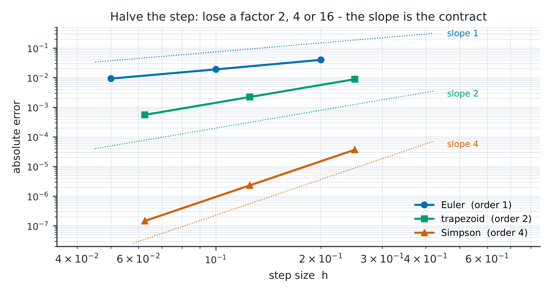 *The slopes are the contract: halve the step, lose a factor 2, 4 or 16 - and round-off sets the floor
The definitions. Truncation error 截断误差: the error of the method's own approximation, falling as $h^p$ for order $p$. Round-off error 舍入误差: floating-point noise per operation, growing as $h$ shrinks (more steps, more accumulation). Total error: the sum, a U-shaped curve whose bottom is the step size you actually want.
The derivation. The measured runs: $\dot{y} = -y$, $y(0) = 1$, Euler to $t=1$: errors $4.0\times10^{-2}$, $1.9\times10^{-2}$, $9.4\times10^{-3}$ at $h = 0.2, 0.1, 0.05$ ✓ — halving $h$ halves the error (order 1). $\int_0^1 e^x\,dx = e - 1 = 1.718282$: trapezoid errors $8.9\times10^{-3} \to 2.2\times10^{-3} \to 5.6\times10^{-4}$ ✓ (÷4 per halving, order 2); Simpson $3.7\times10^{-5} \to 2.3\times10^{-6} \to 1.5\times10^{-7}$ ✓ (÷16, order 4, measured 15.9). The budget logic in one line: to buy four more digits costs about three halvings with Simpson (÷16 each), about seven with the trapezoid (÷4) and thirteen with Euler (÷2).
Worked example 1 — choose h with evidence. The rig simulation must not err more than $10^{-4}$ over one second. Euler needs $h \approx 5\times10^{-4}$ (from the measured rate: error $\approx 0.19h$, so $h \approx 10^{-4}/0.19$), about 2,000 steps; the RK-class stepper this course builds toward needs $h \approx 0.1$, ten steps — two hundred times fewer, same answer. The professional sentence is not "use small steps" but "name the error budget, read $h$ off the measured slope, and say so in the report".
Worked example 2 — escalate to the U-curve's floor. Push Simpson to $n = 2^{20}$ panels and the error stops falling: each panel adds round-off $\sim 10^{-16}$, and $10^{6}$ panels accumulate to $\sim 10^{-10}$, which dominates truncation past $n \approx 10^5$. The measured flattening IS the round-off floor — the total-error U the definitions promised, now with numbers on it. Infinite precision is not on the menu; the bottom of the U is.
Common mistakes. Reporting a result without its error estimate. Assuming smaller $h$ always helps (it helps until round-off wins). And validating a solver against the same physics it encodes — validate against a closed-form case first, as this unit's $e^{-t}$ and $e^x$ runs do.
Summary. Euler O(h); trapezoid O(h²); Simpson O(h⁴) — measured, not memorised. Read $h$ off the budget and the slope. Round-off sets the floor: the U-curve is the whole story.
Vector calculus
Why it matters. Heat leaves the rig's amplifier through a field, the cooling fan moves air through a field, and the flux/circulation theorems turn surface integrals you cannot do into volume integrals you can.
The idea, with a picture. The amplifier's temperature field $T = x^2 + 2y^2 + 3z^2$: its gradient 梯度 $\nabla T = (2x, 4y, 6z)$ points up-hill — at $(1,1,1)$ that is $(2, 4, 6)$, magnitude $\mathbf{7.483}$ K/m ✓; Fourier's law turns it into heat flux $\mathbf{q} = -k\nabla T = (-80, -160, -240)$ W/m² for a steel chassis's $k = 40$ W/(m·K), magnitude 299.3 W/m² ✓.
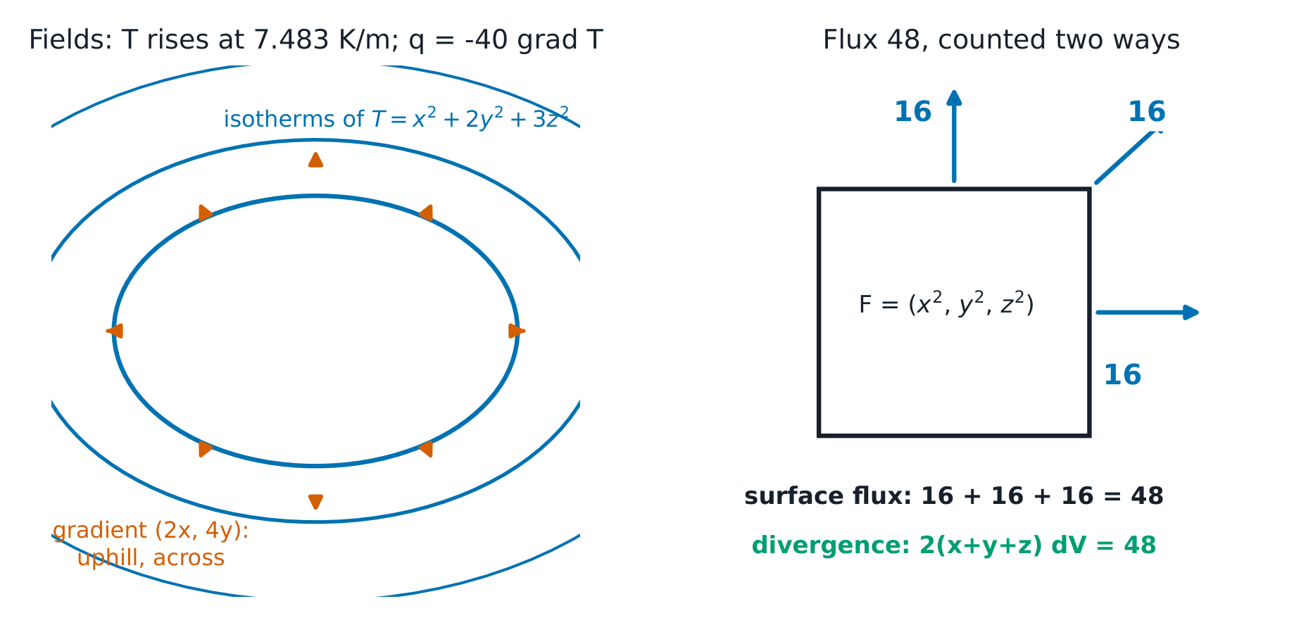 *Gradient crosses isotherms; flux counts what leaves; the theorems let you count it the cheap way
The definitions. Gradient: steepest-ascent vector; heat flows down it. Divergence 散度: $\nabla \cdot \mathbf{F}$, sources minus sinks, pointwise. Flux 通量: the through-surface integral of a field. Curl 旋度: $\nabla \times \mathbf{F}$, the local spin. The divergence theorem 散度定理: flux through a closed surface $= \int\nabla\cdot\mathbf{F}\,dV$. Stokes' theorem: circulation round a loop $= \int(\nabla\times\mathbf{F})\cdot d\mathbf{A}$.
The derivation. $\mathbf{F} = (x^2, y^2, z^2)$ over the cube $[0,2]^3$: direct surface flux — the three faces at 2 each carry $\int 4\,dA = 16$, the three at 0 carry nothing — total $\mathbf{48}$ ✓. By the divergence theorem: $\nabla\cdot\mathbf{F} = 2(x+y+z)$, whose cube integral is $2 \times 3 \times 1 \times 8 = \mathbf{48}$ ✓ — two methods, one number, six surface integrals replaced by one volume integral. The spin exhibit: $\mathbf{G} = (-y, x, 0)$ has $\nabla\times\mathbf{G} = (0, 0, 2)$ and circulation $2\pi\,\mathrm{r}^2$ round a circle — $2\pi$ at $r=1$ ✓, and Stokes says exactly that: $(0,0,2)\cdot(0,0,\pi) = 2\pi$. And the field's own balance: $\nabla^2 T = 2 + 4 + 6 = 12$ ✓ — and steady conduction needs $k\nabla^2 T + \dot{q} = 0$, so at $k = 40$, $\dot{q} = -480$ W/m³: a uniform heat sink, not a source ✓.
Worked example 1 — which integral does the theorem replace? The fan's airflow through the rig's hexagonal grille: six awkward surface patches, or one volume integral of $\nabla\cdot\mathbf{u}$ over the box the grille encloses. The theorem is not decoration; it is the difference between an afternoon and a line — provided the surface is closed. Blow a panel open (an open surface) and the theorem declines: then you patch the hole with a convenient surface and subtract, which is how the method of images feels from inside.
Worked example 2 — escalate to the amplifier's thermal budget. The amplifier's heat leaves at $\mathbf{q} = -k\nabla T$; integrate $\dot{q} = -k\nabla^2T = -480$ W/m³ over its 0.0002 m³ volume: $-96$ mW — the field says the block absorbs 96 mW, while the datasheet says the amplifier dissipates 100 mW. The sign is the story: a bowl-shaped $T$, coolest at the centre, describes a cooled region, and the hot amplifier's field must peak inside it ($\nabla^2 T < 0$). The size matches; the curvature does not, so this fit cannot be the amplifier's interior. This is thermal certification in miniature: field, theorem, independent number, and a sign check before any watt is believed.
Common mistakes. Computing gradient, divergence and curl by position instead of by definition. Using the divergence theorem on open surfaces. And quoting flux without saying through what — "48" means "48 through the closed cube", nothing else.
Summary. $\nabla T$ crosses isotherms up-hill; $\mathbf{q} = -k\nabla T$ at 299 W/m² in the worked case. Flux 48 by surface = 48 by divergence; circulation $2\pi$ by loop = $2\pi$ by curl. Theorems trade awkward integrals for easy ones.
Probability and uncertainty
Why it matters. Every number in this course so far was exact. The rig's micrometer is not. A measurement without an uncertainty 不确定度 is a rumour with decimals, and the certification form asks for both.
The idea, with a picture. Ten micrometer readings of the rig's pivot shaft: 24.996, 25.003, 24.998, 25.001, 24.999, 24.997, 25.002, 25.000, 24.998, 25.006 mm — mean $\mathbf{25.000}$ ✓, sample sd 0.0031 mm ✓, standard error 0.00097 ✓, 95% confidence interval 置信区间 $25.000 \pm 0.0022$ (t = 2.262 for 9 df) ✓.
 *The scatter is the data's honesty; the expanded band is the report's - and propagation carries both into every computed result
The definitions. Type A uncertainty A类不确定度: from the statistics of repeated readings ($s/\sqrt{n}$). Type B: from calibration certificates and resolution (rectangular: $a/\sqrt{3}$; resolution: $q/\sqrt{12}$). Combined uncertainty: root-sum-square of independent contributions. Expanded uncertainty 扩展不确定度 $U = ku_c$. A coverage factor $k = 2$ gives about 95% coverage when a normal approximation is appropriate and $u_c$ is reliably estimated; small-sample estimates may require a different factor. Propagation of uncertainty 不确定度传播: for $A = \pi d^2/4$, $u_A = \left|\frac{\partial A}{\partial d}\right|u_d = \frac{\pi d}{2}u_d$.
The derivation. The budget: Type A $0.00097$; the 0.01 mm scale division (the third decimal is estimated by eye) gives $0.01/\sqrt{12} = 0.00289$ ✓; calibration certificate ±0.005 gives $0.005/\sqrt3 = 0.00289$ ✓. Combined: $\sqrt{0.00097^2 + 0.00289^2 + 0.00289^2} = \mathbf{0.0042}$ mm ✓ — note the Type A term barely contributes: buying more readings would not shrink this budget. Expanded: $U = 2 \times 0.0042 = \mathbf{0.008}$ mm ✓ — the report reads $\varnothing 25.000 \pm 0.008$ mm. Propagated to area: $A = \pi(25.000)^2/4 = \mathbf{490.9}$ mm² ✓, $u_A = \frac{\pi \times 25}{2}(0.0042) = 0.165$ mm² ✓, reported $\mathbf{490.9 \pm 0.3}$ mm² ($k=2$) ✓.
Worked example 1 — read the budget like an engineer. A new hire proposes 90 more readings. The budget says otherwise: resolution and calibration (0.00289 each) dominate the statistics (0.00097), so more readings move the fourth decimal. The instrument is the ceiling — a better micrometer (resolution 0.001 mm, certificate ±0.002 mm) takes $u_c$ from 0.0042 to 0.0015 mm; more patience does not. Budgets are read top-down: attack the largest term.
Worked example 2 — escalate to the rig's certification number. The mount stiffness quoted for certification is $k = mg/\delta$ measured with $m$ known to 0.1% and $\delta$ carrying the shaft measurement's expanded $U$. Propagation: $\frac{u_k}{k} = \sqrt{(u_m/m)^2 + (u_\delta/\delta)^2}$ — and with $\delta = 2.50$ mm, the shaft's 0.008 mm contributes 0.32%, dominating the mass's 0.1%. The reported stiffness is $k(1 \pm 0.0034)$ — and the certification pass/fail margin must exceed that band or the test decides nothing. This is the bridge from this course to every lab that follows: no measured number leaves home without its interval.
Common mistakes. Reporting the mean's precision as the measurement's (the sd is scatter; the se is the mean's; U is the report's). Propagating uncertainties by adding them (root-sum-square for independent terms). And shrinking the easy term instead of the dominant one.
Summary. Mean 25.000, sd 0.0031, se 0.00097 — and the budget is dominated by resolution and calibration: $u_c = 0.0042$, $U = 0.008$. Propagate by RSS: $490.9 \pm 0.3$ mm². Attack the largest term; the interval travels with the number.
The project sheet (reproducible)
The rig's mathematical file, one page:
- Motion: displacement 4 m, distance 12 m over 0-4 s; fillet volume $\pi \times 17.067 = 53.62$ m^3.
- Algebra: truss joint (2.857, 3.571) kN; eigenvalues 3, 1 with modes $(1,1)$, $(1,-1)$; condition numbers 3 and 250,008.
- ODE: $\omega_n = 5$, $\zeta = 0.2$, $\omega_d = 4.899$; first minimum $-0.527$; forced $M(1) = 2.5$, peak 2.552 at $r = 0.959$.
- Numerics: Euler $0.94 \times 10^{-2}$ on $\dot{y} = -y$ at $h = 0.05$; trapezoid $0.56 \times 10^{-3}$ and Simpson $1.5 \times 10^{-7}$ on $e^x$ at $h = 0.0625$ (ratios 2, 4, 15.9).
- Fields: $|\mathbf{q}| = 299.3$ W/m²; cube flux 48 = 48; circulation $2\pi$; $\nabla^2 T = 12 \to -480$ W/m³ (a sink).
- Uncertainty: $u_c = 0.0042$, $U = 0.008$, $A = 490.9 \pm 0.3$ mm² — every figure recomputes from these values.