This is the seventh course in University Electrical Engineering:
electromagnetics 电磁场与波 — the physics under every circuit, antenna and
motor. Circuits hide the fields inside wires; this course opens the box.
Unit 7.1 reviews the vector calculus toolkit (EE02's operators, now with
coordinates and symmetries).
Units 7.2–7.4 build statics: electrostatics, magnetostatics, and the
assembled Maxwell equations.
Units 7.5–7.6 propagate waves and feed them down transmission lines.
Unit 7.7 opens waveguides and antennas.
The running story is one link: a 3 GHz radio connection between two boards
on a bench — its fields, its wave, its cable, its guide, its antennas. Every
field answer below is computed two ways (Gauss vs direct integration; Ampère
vs Biot-Savart), and every wave answer is checked against a limiting case
(free space, perfect conductor, DC).
Why it matters. A phone's GPS receiver hears −130 dBm; whether that
works is decided by divergence and curl. The operators of EE02 are the
grammar; here they take coordinates and learn the symmetry shortcut that
makes real geometry tractable.
The idea, with a picture. A field has an outflow per volume (the
divergence 散度) and a circulation per area (the curl 旋度). Before
touching an integral, test the symmetry of the source: full spherical
symmetry → Gauss's law on a sphere ($dA = r^{2}\sin θ\,dθ\,dφ$);
cylindrical → a coaxial cylinder ($dA = r\,dφ\,dl$); none → direct
integration along the field formula.
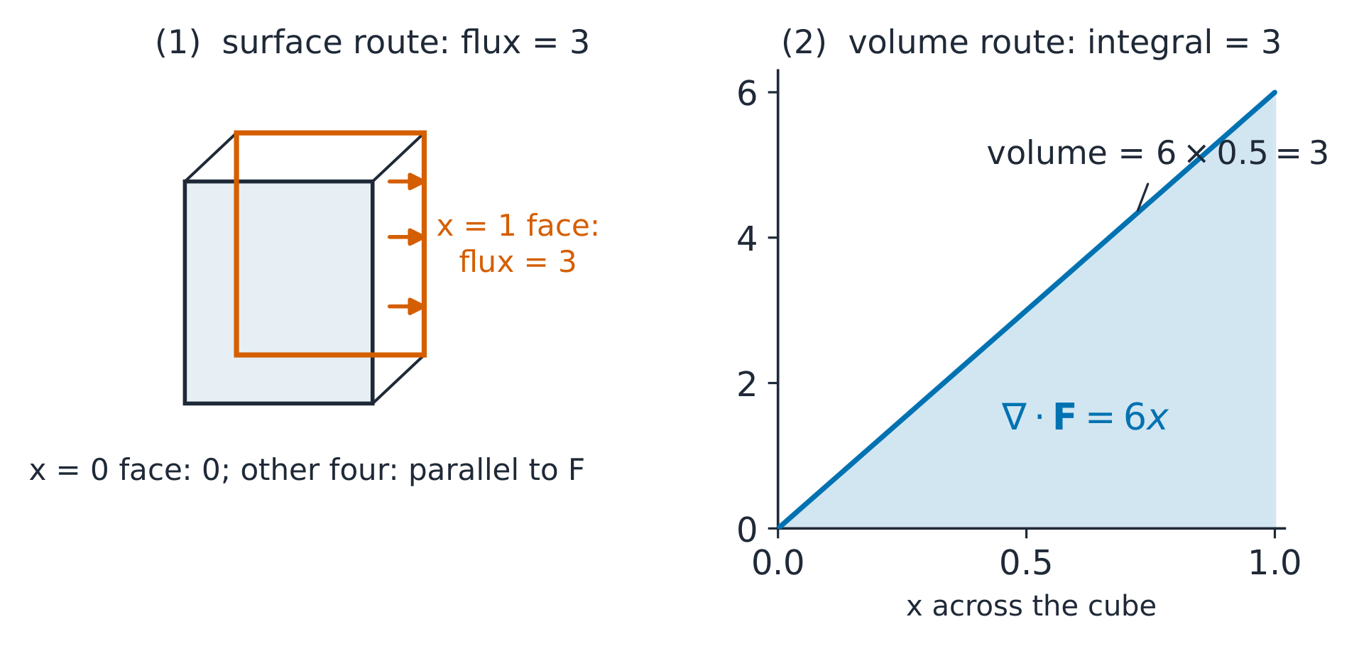
One cube, two routes: integrate 6x over the box, or count the flux through its faces
says the field's net outflow through a closed surface equals the volume
integral of its sources. For a symmetric source, the surface integral
collapses to $E \times A$; solving for the field is then one line — that
one line is every Gauss-law example in this course.
Worked example 1 — divergence with coordinates. Take
$\mathbf{F} = (3x^{2}, 0, 0)$: $\nabla \cdot \mathbf{F} = \partial(3x^{2})/\partial x = 6x$, so at
the point $(2, 0, 0)$ the divergence is 12 per unit volume. Check at the
point $(−2, 0, 0)$: the field still points along $+x$ ($3x^{2}$ is never
negative), yet the divergence is −12 — the sign tracks how the field changes
(the source density), not which way it points.
Worked example 2 — the theorem on a cube. The flux of that $\mathbf{F}$
out of the unit cube $[0,1]^{3}$, by the volume route:
$\int_{0}^{1}\int_{0}^{1}\int_{0}^{1} 6x\,dx\,dy\,dz = 6 \cdot \tfrac{1}{2} = 3$. By
the surface route: only the $x = 1$ face carries flux
($3 \cdot 1 \cdot 1 = 3$; the $x = 0$ face has $3x^{2} = 0$, the four others are
parallel to $\mathbf{F}$) — total 3 ✓. Both routes, one number: the theorem is
an accounting identity you can always afford to check.
Common mistakes. Integrating $r^{2}$ but differentiating $1/r^{2}$
(most Gauss examples hide one such step — write both explicitly). Forgetting
the sphere's $dA = r^{2}\sinθ\,dθ\,dφ$ has an $r^{2}$ that cancels the field's
$1/r^{2}$ — that cancellation IS the method. And applying Gauss's law to
asymmetric sources: no symmetry, no $E \times A$, no shortcut.
Summary. Divergence = outflow density, curl = circulation density;
symmetry chooses the surface; the divergence theorem is the two-route check
that makes every answer here self-verifying.
Explore
A field can point right and still have negative divergence
Start with the worked unit cube and recover total outward flux 3 by both surface and volume routes. Move the box to negative x, where the field still points right but more enters than leaves. A box centred on zero has cancelling source and sink contributions. Compare the local probes at x = 2 and x = −2 to distinguish field direction from divergence sign.
and symmetry converts the integral into arithmetic: for a spherically
symmetric source, $E \cdot 4\pi r^{2} = Q_{enc}/\varepsilon_{0}$.
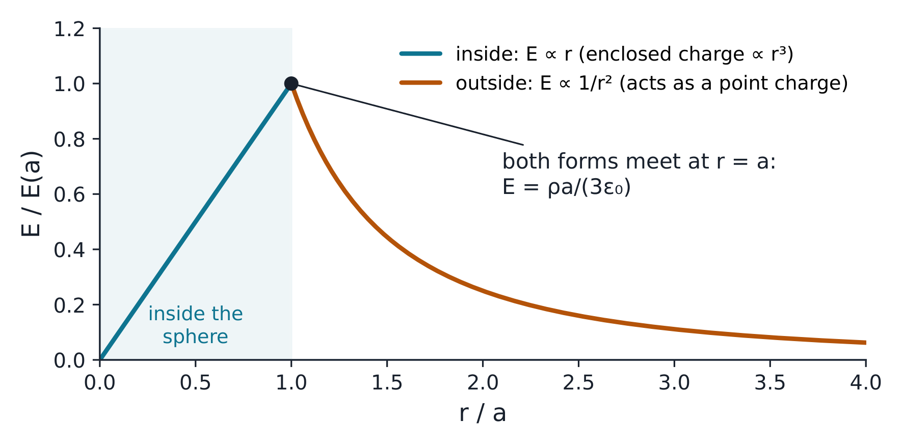
Uniform sphere: E ∝ r inside, E ∝ 1/r² outside, continuous at the surface
The derivation. Inside a uniformly charged sphere of radius $a$ and
density $\rho$, the enclosed charge grows as $r^{3}$ while the Gaussian
sphere's area grows as $r^{2}$:
The potential 电位 stacks the field:
$V(r) = -\int_{\infty}^{r} \mathbf{E} \cdot d\mathbf{l}$; the capacitance 电容 of an
isolated sphere follows, $C = Q/V = 4\pi\varepsilon_{0}a$ — about 1.1 pF per cm
of radius, why free-space objects barely couple. At a dielectric interface
the boundary conditions 边界条件 are: tangential $E$ continuous, normal
$D = \varepsilon E$ jumping by any free surface charge.
Worked example 1 — the sphere, both regions. With $\rho = 1\ \mu\text{C/m}^{3}$
and $a = 2$ cm: at the surface $r = a$, both formulas give
$E = \rho a/3\varepsilon_{0} = (10^{-6} \cdot 0.02)/(3 \times 8.854 \times 10^{-12}) = 753$ V/m ✓
one value, two routes. At $r = 4$ cm (double the radius) the outside form
gives $753/4 = 188$ V/m — the $1/r^{2}$ falloff, one octave out.
Worked example 2 — escalate to the dielectric. Keep the same free
charge density and let a homogeneous, linear dielectric fill all space,
inside and outside the charged region. With $\varepsilon_{r} = 4$, the field
everywhere drops by 4× and the surface value becomes 188 V/m. The
polarisation changes $E$, while $D = \varepsilon E$ is unchanged for the
same free charge. The bound charge inside the sphere is
$Q_{bound} = -(1 - 1/\varepsilon_{r})Q_{free} = -0.75Q_{free}$.
It is distributed through the charged volume. There is no extra bound
surface charge at $r = a$, because the dielectric is the same on both sides
and the polarisation is continuous there. A dielectric sphere surrounded
by vacuum is a different boundary-value problem.
Common mistakes. Using $4\pi r^{2}$ where the geometry is a cylinder
($2\pi r l$). Mixing $\varepsilon_{0}$ and $\varepsilon = \varepsilon_{0}\varepsilon_{r}$ mid-problem —
pick one convention per problem. And applying the outside (point-charge)
form inside the sphere: the enclosed charge, not the total charge, is what
Gauss sees.
Summary. Gauss's law plus symmetry: $E \times A = Q_{enc}/\varepsilon$; the
sphere grows linearly inside, falls as $1/r^{2}$ outside, agrees at the
surface. A dielectric divides fields by $\varepsilon_{r}$ and stores the
difference as bound charge.
Explore
The Gaussian surface counts only the charge inside it
Recover the worked sphere surface field of 753 V/m, then probe half the radius for 377 V/m and twice the radius for 188 V/m. Inside, enclosed charge grows as r cubed and the field rises linearly; outside, charge stays fixed and the field falls as inverse radius squared. Fill all space with the same dielectric and compare E with D. Reverse the free charge to see the field direction change without changing the inside/outside law.
Why it matters. Motors, relays, MRI magnets and every inductor begin
with the same law pair: Biot-Savart for the general case, Ampère when
symmetry is kind.
The idea, with a picture. Currents make fields. Biot-Savart law 毕奥萨伐尔定律 integrates every current element's contribution; Ampère's
law 安培环路定律$\oint \mathbf{B} \cdot d\mathbf{l} = \mu_{0}I_{enc}$ wraps the field
around the current. The symmetry test from Unit 7.1 decides which to use.
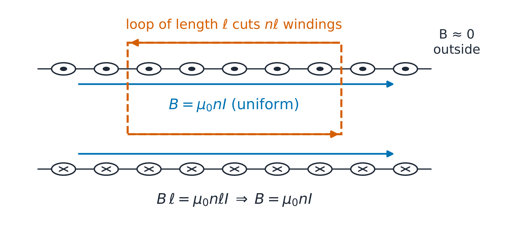
The rectangular Amperian loop cuts the windings; the outside long side contributes zero
The derivation. For an infinite solenoid with $n$ turns per metre,
take a rectangular Amperian loop with one long side inside (length $l$),
one outside, and the short sides crossing the windings. The enclosed
current is $n l I$; the outside field of an infinite solenoid vanishes by
cancellation, and the short sides contribute nothing (field perpendicular to
them). So $B \cdot l = \mu_{0} n l I$:
$$B = \mu_{0} n I \quad \text{(inside, uniform)}, \qquad B \approx 0 \;\; \text{(outside)}.$$
Magnetic flux 磁通量$\Phi = \int \mathbf{B} \cdot d\mathbf{A}$ leads to
inductance 电感$L = N\Phi/I$; for the solenoid, $L/l = \mu_{0}n^{2}A$. The
Lorentz force 洛伦兹力$\mathbf{F} = q\mathbf{v} \times \mathbf{B}$ bends moving charge
into a circle of radius $r = mv/qB$ — the cyclotron orbit.
Worked example 1 — the solenoid priced. With $n = 1000$ turns/m and
$I = 2$ A: $B = 4\pi \times 10^{-7} \times 1000 \times 2 = 2.51$ mT inside, uniform
along the axis. A Biot–Savart check would integrate a thousand loops —
this is why the symmetry test comes first: one line instead of a page.
Worked example 2 — the orbit and the force. A $1\ \mu$C charge at
$10^{6}$ m/s moving perpendicular to a $1$ T field feels
$F = qvB = 10^{-6} \times 10^{6} \times 1 = 1$ N — and circles at radius
$r = mv/qB$: for an electron ($m = 9.11 \times 10^{-31}$ kg),
$r = (9.11 \times 10^{-31} \times 10^{6})/(1.6 \times 10^{-19} \times 1) = 5.7\ \mu$m — the
cyclotron radius that sets magnetron and spectrometer geometry. Check the
speed: an electron at $10^{6}$ m/s carries 2.85 eV — comfortably
non-relativistic, so the formula is honest.
Common mistakes. Forgetting Ampère's law needs the TOTAL enclosed
current (loop with $N$ turns → $NI$). Assuming $\mathbf{B}$ is continuous
across a current sheet (its tangential component jumps by
$\mu_{0}K$). And using the solenoid formula for a short coil: "infinite"
means length ≫ diameter, or the field is weaker and non-uniform.
Summary. Ampère plus symmetry: $B \cdot l = \mu_{0}I_{enc}$; the infinite
solenoid concentrates flux, $B = \mu_{0}nI$, $L/l = \mu_{0}n^{2}A$; moving
charge circles at $r = mv/qB$.
Explore
A long coil is nearly infinite at its centre, not at its ends
Start with the lesson's n = 1000 turns/m and I = 2 A, giving the infinite-coil value 2.51 mT. Compare a chosen finite coil 20 cm long with radius 1 cm, then shorten it to 2 cm while keeping n and I fixed. Probe the centre, end and beyond the end to see where the infinite-solenoid shortcut loses accuracy. Reversing current changes field direction while the geometric reduction stays the same.
The four boxes are a loop: circulating $\mathbf{E}$ makes changing
$\mathbf{B}$, circulating $\mathbf{B}$ makes changing $\mathbf{E}$ — self-sustaining
waves.
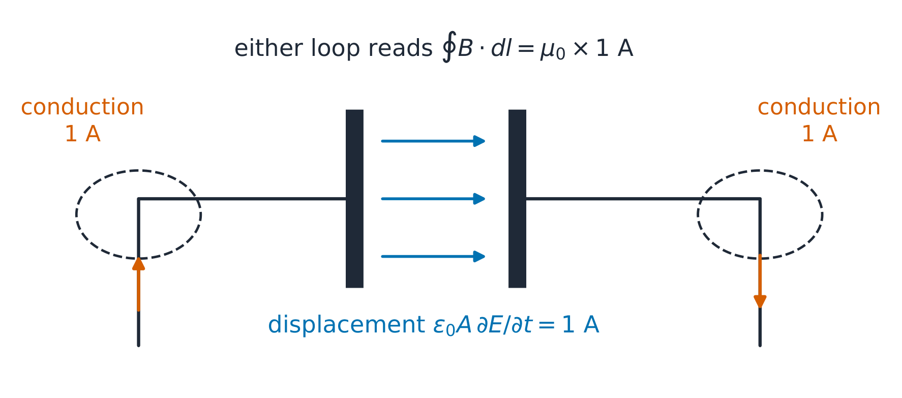
The loop integral cannot depend on which surface you span it with — displacement current makes it true
The derivation. Charge conservation $\nabla \cdot \mathbf{J} = -\partial\rho/\partial t$
forces the correction: take the divergence of the original Ampère law
($\nabla \times \mathbf{B} = \mu_{0}\mathbf{J}$) and the left side is identically zero
while the right side is $-\mu_{0}\partial\rho/\partial t$ — nonzero whenever charge
piles up. Adding $\mu_{0}\varepsilon_{0}\partial\mathbf{E}/\partial t$ repairs it, because
Gauss's law turns that term's divergence into exactly
$+\mu_{0}\partial\rho/\partial t$. The loop closes.
Worked example 1 — the capacitor's missing ampere. A parallel-plate
capacitor charges at $dQ/dt = 1$ A. Between the plates no conduction
current exists, yet an Ampèrian loop around the wire must read the same
1 A whichever surface you span it with. Between the plates
$E = Q/(\varepsilon_{0}A)$, so $\varepsilon_{0}A \cdot \partial E/\partial t = dQ/dt = 1$ A ✓ —
the displacement current IS the conduction current, numerically.
Worked example 2 — escalate to the wave speed. In source-free space
($\rho = 0$, $\mathbf{J} = 0$), take the curl of the $\mathbf{E}$ curl equation and
substitute the $\mathbf{B}$ one:
the wave equation with speed $c = 1/\sqrt{\mu_{0}\varepsilon_{0}}$. Insert the
numbers: $1/\sqrt{\mu_{0}\varepsilon_{0}} = 3.0 \times 10^{8}$ m/s — light,
from two constants measured on a bench. The link budget of the
running story begins here.
Common mistakes. Treating displacement current as optional bookkeeping
(it is what makes the equations consistent and what carries the wave).
Forgetting which equation has the minus sign (Faraday's: it is Lenz's law,
the induced field opposing the change). And applying the static
forms to antennas: radiation IS the correction term doing its work.
Summary. Four equations, one loop; displacement current closes charge
conservation and, in vacuum, yields the wave equation at
$c = 1/\sqrt{\mu_{0}\varepsilon_{0}}$.
Explore
Same loop, two surfaces; Maxwell supplies the missing ampere
Start with the worked charging current of 1 A and compare a surface cutting the wire with one passing through the vacuum gap. The original law gives different predictions; including the changing-electric-flux term makes both totals equal. Change plate area to alter the field rate while its product with ε₀A remains the same current. Hold a nonzero stored charge to distinguish electric field from changing electric field.
Why it matters. Wi-Fi, radar, sunlight and the bench link's 3 GHz
carrier are all the same solution: the plane wave.
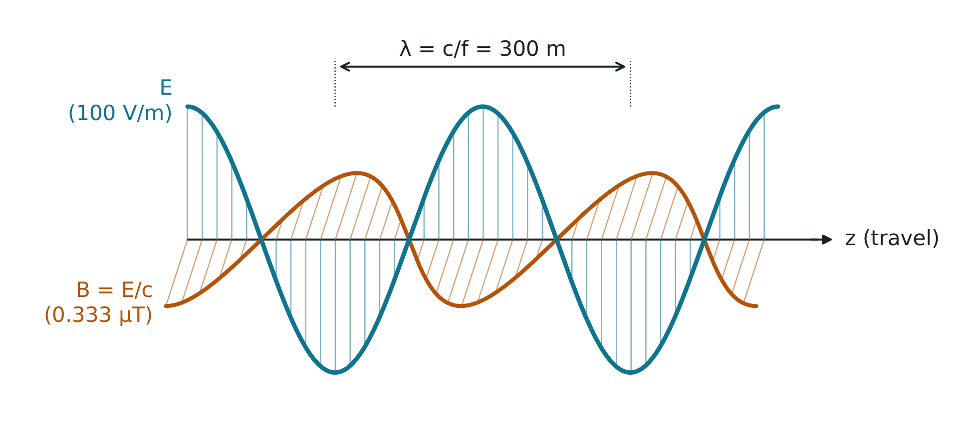
The idea, with a picture. In source-free space the wave equation's
simplest solution is a plane wave 平面电磁波: $\mathbf{E}$, $\mathbf{B}$ and the
propagation direction mutually perpendicular, in phase, with
$B = E/c$. The intrinsic impedance 波阻抗$\eta_{0} = \sqrt{\mu_{0}/\varepsilon_{0}} = 377\ \Omega$ of free space sets the ratio of
$E$ to $H$; the Poynting vector 坡印亭矢量$\mathbf{S} = \mathbf{E} \times \mathbf{H}$
points along the propagation with $S = E^{2}/\eta_{0}$ (instantaneous; with rms
values of $E$ this is the average power density, while a sinusoid of amplitude
$E_{0}$ averages $E_{0}^{2}/2\eta_{0}$).
E and B in phase and at right angles; λ = 300 m at 1 MHz
The derivation. For $\mathbf{E} = E_{0}\cos(\omega t - kz)\,\hat{x}$, Faraday's
law gives $\partial B/\partial t = -\partial E/\partial z$, integrating to
$B = (k/\omega)E = E/c$. The power density follows from the impedance:
$H = E/\eta_{0}$, so $S = E \times H = E^{2}/\eta_{0}$ — one number per wave.
Worked example 1 — reading the numbers off. A 100 V/m (rms) wave at 1 MHz:
$B = 100/(3 \times 10^{8}) = 0.333\ \mu$T; wavelength
$\lambda = c/f = 300$ m; power density $S = 100^{2}/377 = 26.5$ W/m². Check
the impedance route: $H = 100/377 = 0.265$ A/m, and $E \times H = 26.5$ ✓ —
the two routes agree because they are the same ratio.
Worked example 2 — escalate to the conductor's skin. In a good
conductor 良导体 the wave decays as $e^{-\alpha z}$ with skin depth 趋肤深度$\delta = \sqrt{2/(\omega\mu\sigma)}$. Copper ($\sigma = 5.8 \times 10^{7}$): at 50 Hz,
$\delta = \sqrt{2/(2\pi \cdot 50 \cdot 4\pi \times 10^{-7} \cdot 5.8 \times 10^{7})} = 9.3$ mm;
at 1 GHz, $\delta = 2.1\ \mu$m — about 4500 times thinner for twenty
million times the frequency ($\delta \propto 1/\sqrt{f}$ ✓). This one number
explains why shields work, why RF current rides the surface, and why the
bench link's 3 GHz traces need wide, smooth copper: at 3 GHz the current lives
in the top 1.2 µm, so surface roughness and any plating there set the loss (gold
plating protects against corrosion; it conducts worse than copper).
Common mistakes. Using $c$ in a dielectric — the speed there is
$1/\sqrt{\mu\varepsilon}$ (≈ 0.67c in the coax below). Mixing $E/H$ (377 Ω in
space) with $E/B$ ($c$ — a speed, not an impedance). And forgetting the
wave's fields are in phase in a LOSSLESS medium only.
Summary. Plane wave: $E \perp B \perp \hat{k}$, $B = E/c$,
$S = E^{2}/\eta_{0}$; conductors eat waves as $e^{-z/\delta}$ with
$\delta = \sqrt{2/\omega\mu\sigma}$.
Start with the worked 100 V/m RMS wave at 1 MHz. Its average power is about 26.5 W/m², while its instantaneous power at a field crest is twice that. Reinterpret the same number as a peak field and the average halves. Advance half a cycle to reverse E and H together without reversing the Poynting vector. Compare a uniform dielectric to vacuum, keeping the entered electric field specified.
Why it matters. The bench link's two boards are joined by 40 cm of
coax; at 3 GHz that is six wavelengths — a circuit no more, a
transmission line.
The idea, with a picture. The telegrapher equations 电报方程 treat
the line as distributed inductance $L'$ and capacitance $C'$ per metre:
$\partial v/\partial x = -L'\partial i/\partial t$ and
$\partial i/\partial x = -C'\partial v/\partial t$. Their solutions are voltage/current
waves with $v_{p} = 1/\sqrt{L'C'}$ and the line's characteristic impedance
特性阻抗$Z_{0} = \sqrt{L'/C'}$.
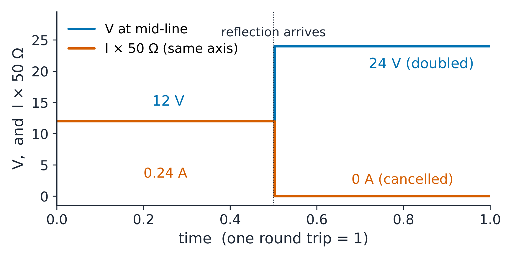
The open-end signature: voltage doubles, current goes to zero
The derivation. Differentiate the first equation in $x$ and the second
in $t$ and eliminate $\partial^{2}i/\partial x \partial t$: a wave equation for $v$
with speed $1/\sqrt{L'C'}$. At a load $Z_{L}$, matching gives the
reflection coefficient $\Gamma = (Z_{L} - Z_{0})/(Z_{L} + Z_{0})$: a short
($\Gamma = -1$) inverts, an open ($\Gamma = +1$) doubles the voltage and
cancels the current — the bounce diagram 反弹图 tracks every bounce.
Worked example 1 — a real coax. RG-316-class coax with
$L' = 250$ nH/m and $C' = 100$ pF/m:
$Z_{0} = \sqrt{250 \times 10^{-9}/100 \times 10^{-12}} = \sqrt{2500} = 50\ \Omega$ ✓ (the
standard cable — the numbers were chosen to make it so);
$v_{p} = 1/\sqrt{250 \times 10^{-9} \times 100 \times 10^{-12}} = 2 \times 10^{8}$ m/s =
0.67c. The bench link's 40 cm of it is SIX wavelengths at 3 GHz
($\lambda = v_{p}/f = 6.7$ cm) — proving the "line, not circuit" point with
the parts on the bench.
Worked example 2 — the open-ended step. Drive that 50 Ω line with a
12 V step, open-ended. The incident wave carries 12 V and
$12/50 = 0.24$ A. At the open, $\Gamma = +1$: the reflected +12 V doubles
the load voltage to 24 V and the reflected current $-0.24$ A cancels the
forward current to zero — an open circuit draws no steady current ✓, and
the VSWR tends to infinity, the open-circuit signature the standing-wave
meter reads.
Common mistakes. Using $Z_{0}$ as a physical resistance (it is a
ratio; a lossless 50 Ω line dissipates nothing). Computing $\lambda$ with
$c$ instead of $v_{p}$ (30% error in PTFE). And forgetting the source-side
reflection: a mismatched driver re-reflects, and the bounce diagram must
include it.
Summary.$Z_{0} = \sqrt{L'/C'}$, $v_{p} = 1/\sqrt{L'C'}$;
$\Gamma = (Z_{L}-Z_{0})/(Z_{L}+Z_{0})$; opens double voltage, shorts cancel it;
long lines are waves, and the bounce diagram is the bookkeeping.
A 24 V source with 50 Ω series resistance launches the worked 12 V incident step. Follow its finite propagation delay to the open load, where voltage doubles and current cancels. Compare a short and a matched load, then change the source resistance to see whether the returning wave is absorbed or reflected again.
Why it matters. Above ~10 GHz coax loses too much; the bench link's
backhaul (and every radar) moves into hollow pipe, and the last metre of
any radio link is always an antenna.
The idea, with a picture. A hollow conducting pipe guides waves only
above the cutoff 截止频率 frequency: the rectangular guide's dominant
mode cuts off at $f_{c} = c/(2a)$ ($a$ = wide dimension). Above cutoff the
guide wavelength 波导波长 stretches:
$\lambda_{g} = \lambda/\sqrt{1 - (f_{c}/f)^{2}}$ — the wave zigzags, so fewer axial
cycles fit per metre of pipe. Antennas close the link: the half-wave
dipole 偶极子天线 has gain 2.15 dBi and input resistance ≈ 73 Ω; the
Friis equation 弗里斯方程 prices the whole link:
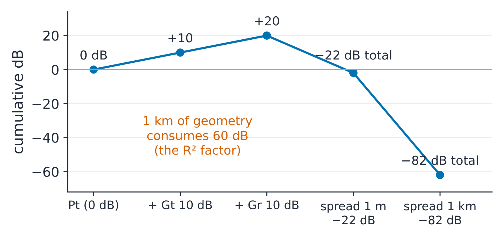
Every dB in the chain is a design decision; the last term is pure geometry
The derivation. Between the plates of the guide, the field must fit a
standing half-wave across $a$: $a = \lambda_{c}/2$ at cutoff, so
$f_{c} = c/2a$. Along the guide, the propagation constant satisfies
$k_{g}^{2} = k^{2} - (\pi/a)^{2}$; solving for the wavelength gives the
stretch formula above. The Friis chain multiplies: transmit power × both
gains × the spreading factor $(\lambda/4\pi R)^{2}$ — an area ratio, the
antenna aperture over the sphere's area.
Worked example 1 — WR-90 at X-band. WR-90 waveguide has
$a = 22.86$ mm: $f_{c} = 3 \times 10^{8}/(2 \times 0.02286) = 6.56$ GHz — X-band
(8.2–12.4 GHz) rides above cutoff. At 10 GHz ($\lambda = 30$ mm):
$\lambda_{g} = 30/\sqrt{1 - 0.656^{2}} = 39.8$ mm — 33% longer than free space.
Check the limit: as $f \to f_{c}$, $\lambda_{g} \to \infty$ (the wave stops);
as $f \to \infty$, $\lambda_{g} \to \lambda$ (the zigzag vanishes) ✓.
Worked example 2 — the bench link's budget. Two 10-dBi (G = 10)
antennas, 1 m apart on the bench, at 3 GHz ($\lambda = 0.1$ m):
$P_{r}/P_{t} = 10 \times 10 \times (0.1/(4\pi \times 1))^{2} = 100 \times 6.33 \times 10^{-5} = 6.3 \times 10^{-3}$ —
22 dB of loss, still easy on the bench. Scale to the same boards 1 km
apart: $(0.1/(4\pi \times 1000))^{2} = 6.33 \times 10^{-11}$, times 100 =
$6.3 \times 10^{-9}$ (−82 dB) — the link budget that decides dish sizes. One
formula, two scales, and the ratio between them is pure geometry
($R^{2}$, a factor of $10^{6}$ ✓).
Common mistakes. Using the guide's NARROW dimension for $f_{c}$ (cutoff
is set by the wide one). Applying $\lambda_{g}$ as if it were $\lambda$ in Friis
(the free-space wavelength belongs there). And quoting dipole gain in dB
without the "i": 2.15 dBi is relative to isotropic; relative to a dipole
it is zero.
Summary. Guide: $f_{c} = c/2a$, $\lambda_{g} = \lambda/\sqrt{1-(f_{c}/f)^{2}}$
(stretched, infinite at cutoff). Antennas: Friis
$P_{r}/P_{t} = G_{r}G_{t}(\lambda/4\pi R)^{2}$ — geometry decides the last term
every time.
Explore
A transverse half-wave decides whether the mode travels
Start with WR-90 at 10 GHz and compare its 39.8 mm guide wavelength with the 30 mm free-space wavelength. Change the wide dimension and frequency to cross cutoff. The transverse field still fits the walls, but the axial pattern changes from a travelling wave to a decaying field. Near cutoff, its phase spacing becomes very long.