This is the fifth course in University Electrical Engineering: electronics I模拟电子学 — the first course on devices. Wave 1 and EE04 analysed circuits made
of ideal components; here the components themselves are the subject, and the
core skill is modelling 建模: choosing the simplest device model that answers
the question at hand.
Unit 5.1 introduces semiconductors and the diode's ladder of models.
Unit 5.2 applies diodes: rectifiers, supplies and zener regulators.
Units 5.3–5.4 bias the two transistor families (BJT, MOSFET).
Unit 5.5 linearises about the bias point: small-signal amplifiers.
Units 5.6–5.7 add feedback and the frequency-domain view.
The checking habit: every bias point is verified against the device's
operating regions (the assumption that made the equation legal), every
small-signal answer at a limiting case. Each unit ends with the common
mistakes and a three-line summary.
Pure silicon conducts poorly; doping 掺杂 adds carriers — donors make n-type
(electrons), acceptors make p-type (holes). A pn junction PN 结 conducts one
way: forward bias (p side positive) lets current flow exponentially; reverse
bias widens the depletion region and blocks.
The diode has a ladder of models — pick by the question:
Ideal 理想模型: 0 V when conducting, open when off.
Constant-drop 恒压降模型: 0.7 V when conducting (silicon).
Piecewise-linear 折线模型: 0.7 V + slope resistance $r_{d} = nV_{T}/I_{D}$.
The exponential 指数模型 Shockley law $i = I_{S}(e^{v/nV_{T}} - 1)$ when the
curve shape matters, with $V_{T} = kT/q \approx 26$ mV at room temperature.
Why the ladder works: differentiate the Shockley law at the operating point
and the diode's dynamic resistance is $r_{d} = nV_{T}/I_{D}$ — a few ohms at
milliamps. And because $i \propto e^{v/nV_{T}}$, ten times the current needs
only $\ln 10 \times nV_{T} = 2.303 \times 26 = 59.9$ mV more voltage (n = 1):
the curve is a near-vertical wall, so the resistor in the loop, not the
diode, sets the current — which is exactly when the constant-drop model is
accurate.
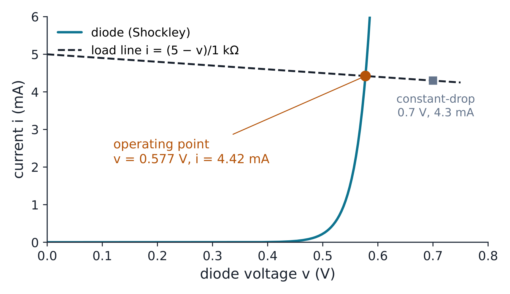
The load line fixes the current; the steep diode curve barely moves the voltage
Worked example 1 (model selection, three ways). A 5 V source feeds a diode
in series with 1 kΩ. Ideal: 5 mA. Constant-drop: $(5 - 0.7)/1000 = 4.3$ mA.
Shockley truth ($I_{S} = 10^{-12}$ A, $nV_{T} = 26$ mV, bisection on
$I_{S}(e^{v/26\mathrm{m}} - 1) = (5 - v)/1000$): $v_{D} = 0.5775$ V,
$i = 4.423$ mA. The constant-drop answer is within 2.8% — because the resistor
dominates the loop. Check why: the constant-drop model is off by
$0.7 - 0.5775 = 0.12$ V in the diode voltage, and the resistor turns that into
only $0.12/1000 = 0.12$ mA of current error — 2.8% of 4.42 mA.
Worked example 2 (the dynamic resistance, escalated). At that operating
point $r_{d} = nV_{T}/I_{D} = 26\,\mathrm{mV}/4.42\,\mathrm{mA} = 5.9\ \Omega$.
Now let the source wiggle by $\pm 0.1$ V (small signal): the wiggle current is
$0.1/(1000 + 5.9) = 99.4\ \mu\mathrm{A}$ — within 0.6% of the resistor-only
100 µA. The 5 V worth of DC sits across the pair almost unchanged; the 0.1 V
of signal sees an ordinary $1\ \mathrm{k}\Omega + 5.9\ \Omega$ loop. This is the whole
small-signal idea of unit 5.5, met first at the diode: split the problem into
a bias (where the nonlinear law sets the point) and a wiggle (where the
linearised resistance takes over).
Common mistakes. Using the exponential model when the resistor dominates
(needless bisection; the constant-drop model is the right tool there).
Quoting "$r_d$ = 26 mV" — that is $V_T$; the resistance is $V_T/I_D$, current
in the denominator. Forgetting n = 2 at high current (59.9 mV/decade becomes
120 mV/decade).
Summary: a diode is a one-way valve with a near-vertical forward curve; the
loop resistor sets the current; $r_d = nV_T/I_D$ is the linearised view; pick
the model the question needs and check the answer against the next model up.
Explore
Find the bias point, then test a small change
$V_s=RI_D+v_D,\quad r_d\approx\frac{nV_T}{I_D}$
The 5 V and 1 kΩ circuit gives about 0.5775 V and 4.42 mA with Shockley, compared with 4.3 mA for the 0.7 V model. Change the source or resistor, then compare a +0.1 V source change with the local dynamic-resistance prediction. A low-supply case shows why a fixed drop can fail.
The half-wave rectifier 半波整流器 conducts one half-cycle; the full-wave
bridge 桥式整流 conducts both (four diodes, two conducting at a time, so the
diode drops cost 1.4 V and each diode must survive a peak inverse voltage反向峰值电压 of one secondary peak). A filter capacitor 滤波电容 holds the
output between peaks: the ripple 纹波$\Delta V \approx I_{load}/(f\cdot C)$
(half-wave) or $I_{load}/(2f\cdot C)$ (full-wave) — the capacitor must supply
the load for the whole gap between recharge peaks.
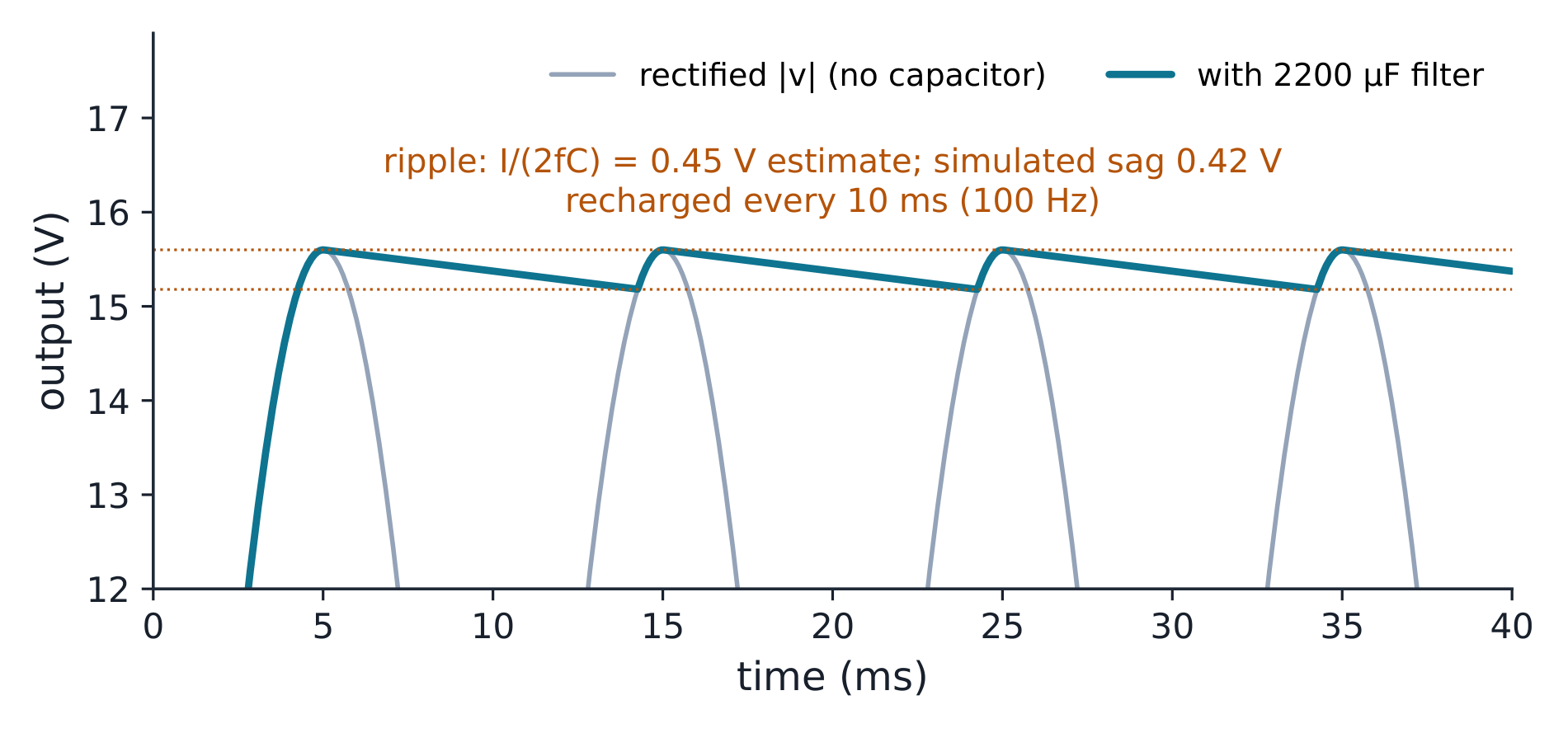
Full-wave bridge with 2200 µF at 100 mA: the capacitor bridges the gaps between peaks
Worked example 1 (the bridge supply, checked). A bridge rectifies a 12 V
RMS, 50 Hz secondary; the load draws 100 mA and the capacitor is 2200 µF.
Peak output: $12\sqrt{2} - 1.4 = 17.0 - 1.4 = 15.6$ V. Ripple (full wave,
recharged every 10 ms): $\Delta V = 0.1/(100 \times 2200\mu) = 0.455$ V. So the
output lives between 15.6 and 15.1 V. Checks: ripple ≪ peak (2.9% ✓ — the
formula's premise); half-wave would double the ripple to 0.91 V for the same
capacitor — the bridge buys a 2× for four diodes; PIV per diode ≈ 17.0 V (one
secondary peak) — rate the diodes above that.
Worked example 2 (a zener regulator designed at both extremes, escalated).
Regulate 12 V down to 5.1 V with a 5.1 V zener 齐纳二极管; the load varies
0–10 mA and the zener needs at least 2 mA to stay in breakdown. Worst case for
the zener current is full load: $R \le (12 - 5.1)/(10\mathrm{m} + 2\mathrm{m}) = 575\ \Omega$ → pick
560 Ω. Now check the other extreme — no load: $I_{Z} = (12 - 5.1)/560 =
12.3$ mA, so $P_{Z} = 5.1 \times 12.3\mathrm{m} = 63$ mW and the resistor
dissipates $(12-5.1)^{2}/560 = 85$ mW worst case. Full load leaves $I_{Z} =
12.3 - 10 = 2.3$ mA ≥ 2 mA ✓. Both extremes verified — that is a complete
regulator design: one inequality from each end of the load range.
Common mistakes. Using f instead of 2f for the bridge ripple (the
capacitor recharges every half-cycle). Forgetting the 1.4 V of two diode drops
in the peak output. Sizing the zener resistor at the typical load only —
the zener current must be checked at BOTH extremes, and its power at the
no-load extreme.
Summary: bridge = both half-cycles, 1.4 V cost, PIV one peak; ripple
$I/(2fC)$ set by the gap between recharges; the zener holds the voltage while
the series resistor absorbs the surplus — designed at the two load extremes.
Explore
One resistor, two opposite design limits
$I_Z=\frac{V_{in}-V_Z}{R}-I_L$
For the 12 V to 5.1 V example, 560 Ω leaves 2.32 mA for the zener at a 10 mA load and about 63 mW at no load. With an illustrative 100 mW power rating, compare the lower power-bound resistance with the 575 Ω upper current bound. A smaller resistor can exceed the power rating; a larger one can lose regulation.
The bipolar junction transistor 双极型晶体管 has three regions — cut-off,
active 放大区 (the amplifier region: $I_C = \beta I_B$, $V_{BE} \approx 0.7$ V),
and saturation ($V_{CE} < 0.2$ V, both junctions forward). Biasing means
placing the quiescent point (the bias point 工作点, Q-point) firmly in the
active region and making it independent of β — the parameter that varies 2:1
between devices of the same part number.
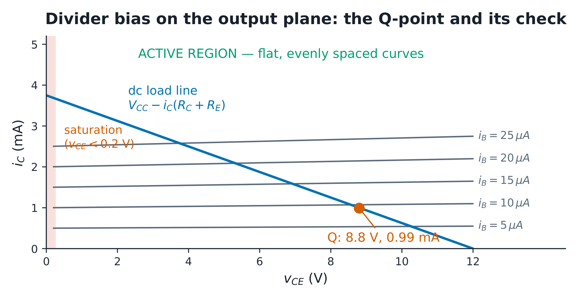
The 12 V dc load line (RC + RE = 3.2 kΩ) with the divider-bias Q-point at 0.99 mA, 8.8 V
Worked example 1 (voltage-divider bias, exact).$V_{CC} = 12$ V;
$R_{1} = 68$ kΩ (to $V_{CC}$), $R_{2} = 12$ kΩ (to ground), $R_{C} = 2.2$ kΩ,
$R_{E} = 1$ kΩ, $\beta = 100$. Thévenin the divider: $V_{B} = 12 \times
12/80 = 1.8$ V, $R_{B} = 68\mathrm{k} \parallel 12\mathrm{k} = 10.2$ kΩ.
Quick estimate (ignore base current): $V_{E} = 1.8 - 0.7 = 1.1$ V →
$I_{E} \approx 1.1$ mA. Exact (base loop with $I_E = (\beta+1)I_B$):
$I_B = (1.8 - 0.7)/(10.2\mathrm{k} + 101 \times 1\mathrm{k}) = 9.9\ \mu$A →
$I_C = 0.989$ mA, $V_{CE} = 12 - 0.99\mathrm{m} \times 2.2\mathrm{k} - 0.99 =
8.8$ V — active ✓ ($V_{CE} \gg 0.2$ V). The quick estimate was 11% high; the
culprit is base current loading the divider — exactly what the exact loop
accounts for.
Worked example 2 (β doubled, the point of the circuit, escalated). Same
circuit, $\beta = 200$: $I_B = 1.1/(10.2\mathrm{k} + 201\mathrm{k}) =
5.2\ \mu$A → $I_C = 1.04$ mA, $V_{CE} = 8.7$ V — still active ✓. So β × 2
moved the collector current by 5% (0.99 → 1.04 mA) and the Q-point barely
budged. The mechanism: any collector-current rise pushes the emitter voltage
up, which reduces$V_{BE}$ and throttles the base current — negative
feedback inside the bias, provided by $R_E$. With $R_E = 0$, the active-region
formula $I_C = \beta(1.8 - 0.7)/10.2\mathrm{k}$ predicts 10.8 mA at β = 100
and 21.6 mA at β = 200. The 2.2 kΩ collector resistor cannot pass either
current from 12 V, so the active assumption fails: these are candidates,
not actual saturated currents. The formula's β sensitivity is still clear,
but the region check must come before accepting a Q-point. Both error sources are now quantified: 11% from divider
loading (fixable with a stiffer divider), 5% from β spread (absorbed by
$R_E$).
Common mistakes. Checking $V_{CE} > 0$ instead of $> 0.2$ V (saturation
starts at about 0.2 V). Computing $V_C$ from the estimated 1.1 mA and then
"checking" against a Q-point computed from the exact current — carry one
chain, then check it. Believing the divider alone makes the bias independent
of β — it is $R_E$ (with the divider stiff enough to hold $V_B$) that does
the work.
Summary: Thévenin the divider, solve the base loop exactly, check the region;
$R_E$ buys β-independence at the price of headroom; estimate-then-verify is
fine when the two are labelled as such.
Explore
A doubled β does not have to double the current
$I_B=\frac{V_{TH}-0.7}{R_{TH}+(\beta+1)R_E}$
Keep the worked 12 V, 68 kΩ/12 kΩ divider, 2.2 kΩ collector resistor and 1 kΩ emitter resistor. Compare β = 100 and 200, then remove the emitter resistor or stiffen the divider. Check the active assumption before accepting any current or voltage as a Q-point.
The MOSFET 金属氧化物半导体场效应晶体管 is voltage-controlled: the gate
draws no DC current, and in saturation 饱和区 (the amplifier region — the
opposite naming to the BJT!) the square-law model 平方律模型 gives
with threshold 阈值$V_t$. The three regions: cut-off ($v_{GS} < V_t$),
triode/ohmic ($v_{DS} < v_{GS} - V_t$ — a resistor, not an amplifier),
saturation (the inequality holds — a current source).
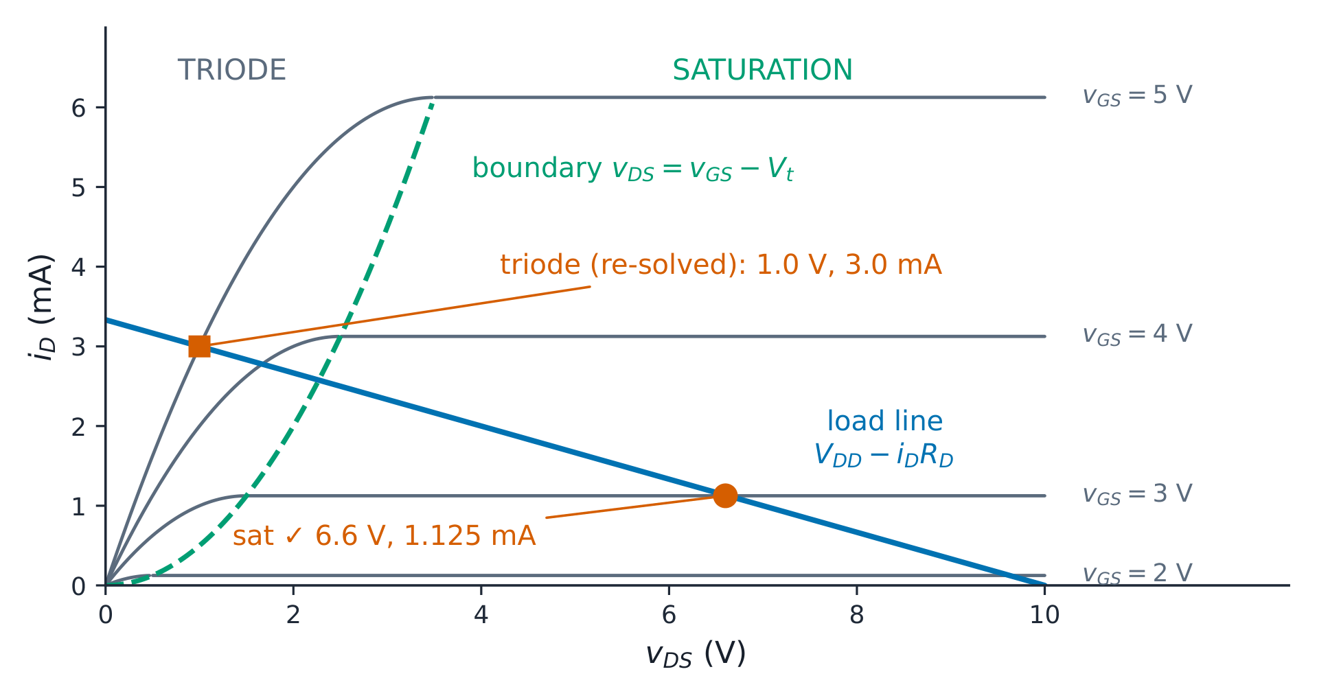
The boundary parabola vDS = vGS − Vt is the region test; both worked examples sit on this map
Worked example 1 (assume saturation, then check).$V_{DD} = 10$ V,
$\tfrac{1}{2}k_n(W/L) = 0.5$ mA/V², $V_t = 1.5$ V, $R_D = 3$ kΩ, gate held at
$V_G = 3$ V (divider — no DC gate current). Assume saturation:
$I_D = 0.5 \times (3 - 1.5)^{2} = 1.125$ mA; $V_{DS} = 10 - 1.125\mathrm{m}
\times 3\mathrm{k} = 6.6$ V. Check: $6.6 \ge 3 - 1.5 = 1.5$ ✓ — saturation
stands, and the Q-point is (1.125 mA, 6.6 V).
Worked example 2 (the check that fails, escalated). Raise the gate to
$V_G = 5$ V, same circuit. Assume saturation: $I_D = 0.5 \times 3.5^{2} =
6.1$ mA, $V_{DS} = 10 - 6.1\mathrm{m} \times 3\mathrm{k} = -8.4$ V —
impossible (negative drain voltage), so the assumption is dead: the resistor
cannot drop 18 V from a 10 V rail. Re-solve in triode with
$i_D = 0.5(2 \times 3.5\, v_{DS} - v_{DS}^{2})$ and the load line
$10 = 3\mathrm{k}\, i_D + v_{DS}$: the quadratic gives $v_{DS} = 1.00$ V,
$i_D = 3.00$ mA. Checks: region $1.0 < 3.5$ ✓ triode; the triode equation
returns $0.5(2 \times 3.5 \times 1 - 1) = 3.0$ mA ✓ consistent with the load
line; and saturation at this gate would have demanded 18.4 V of supply. The
lesson generalises: the model is an assumption — the region check is what
makes it legal.
Common mistakes. Trusting the saturation current without the region
check (the failed example above sails through to a wrong answer if you only
check $V_{DS} > 0$). Mixing up the region names with the BJT (MOSFET
saturation = amplifier; BJT saturation = ruined). Forgetting the gate
current is zero at DC — the divider is unloaded, which is precisely why
MOSFET dividers can use megohm resistors.
Summary: square law in saturation, boundary $v_{DS} = v_{GS} - V_t$ is the
test; assume, solve, check — and when the check fails, the triode quadratic
takes over; gate current zero at DC.
Explore
The region check chooses the operating point
$V_{DS}\ge V_{GS}-V_t\quad\text{for saturation}$
The worked 3 V gate gives a valid saturation point at 1.125 mA and 6.625 V. At a 5 V gate the saturation assumption fails, and the triode equation has two algebraic roots. Only 1 V and 3 mA satisfies the assumed region; the larger positive root is rejected.
Amplification is linear only about a bias point (the Q-point of unit 5.3).
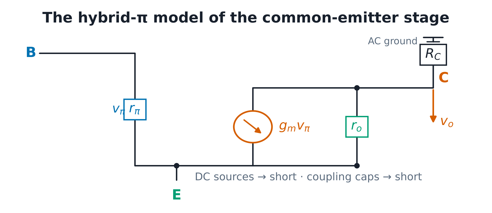
The small-signal 小信号 model replaces each device by its linearised
parameters at that point: BJT — $g_m = I_C/V_T$ (differentiate the
exponential), $r_\pi = \beta/g_m$, $r_o$; MOSFET — $g_m = k(W/L)(V_{GS} -
V_t) = 2I_D/(V_{GS} - V_t)$ (differentiate the square law), $r_o$. DC sources
become shorts; coupling capacitors become shorts at signal frequency.
One linear circuit answers every small-signal question about the stage
Worked example 1 (the common-emitter stage). At the unit-5.3 bias point
$I_C = 0.99$ mA, $\beta = 100$: $g_m = 0.99\mathrm{m}/26\mathrm{m} = 38.1$
mS; $r_\pi = 100/38.1\mathrm{m} = 2.6$ kΩ. Voltage gain with $R_E$ bypassed
and $r_o = 50$ kΩ: $A_v = -g_m(R_C \parallel r_o) = -38.1\mathrm{m} \times
2.11\mathrm{k} = -80$. Limiting checks: $r_o \to \infty$ gives $-g_m R_C =
-84$ (r_o costs 5%); and the gain must be negative — the CE stage inverts.
Worked example 2 (degeneration and the MOSFET comparison, escalated).
Lift the bypass so $R_E = 1$ kΩ participates: the exact gain is
$-g_m R_C/(1 + g_m R_E) = -84/(1 + 38.1) = -2.14$, against the $-R_C/R_E =
-2.2$ textbook form — within 2.4% because $g_m R_E = 38 \gg 1$ (that is the
form's validity condition, now visible). Degeneration traded 84 for 2.2 —
linearity and a stable gain bought with the same $R_E$ that stabilised the
bias. Same story in MOSFET land: the unit-5.4 Q-point gives $g_m = 2I_D/V_{ov} =
2 \times 1.125\mathrm{m}/1.5 = 1.5$ mS and a common-source gain
$-g_m R_D = -4.5$. The BJT at the same 1.125 mA has $43.3$ mS — 29× the
MOSFET's — transconductance and current gain versus infinite input
resistance: the fundamental trade.
Common mistakes. Computing $g_m$ from the estimated bias current after
the exact solve exists — one chain, one set of parameters. Using
$-R_C/R_E$ where $g_m R_E \sim 1$ (the form needs $g_m R_E \gg 1$).
Believing the small-signal model is a different circuit — it is the same
circuit, differentiated at the Q-point.
Summary: differentiate the device law at the Q-point to get $g_m$;
$r_\pi = \beta/g_m$; bypassed gain $-g_m R_C$, degenerated $-R_C/R_E$ when
$g_m R_E \gg 1$; the BJT wins gm-per-milliamp, the MOSFET wins the gate.
Explore
A small-signal model is a tangent at the bias point
Start with the worked 0.99 mA BJT bias and recover gm about 38.1 mS, input resistance about 2.6 kΩ and bypassed gain about −80. Widen the input excursion to see the curved current law leave its tangent. Switch device at the same bias current to compare gm fairly, then select the MOSFET worked bias of 1.125 mA for gm 1.5 mS and gain −4.5.
Wave 1's golden rules return with the finite-gain view. Negative feedback
closes a loop; what matters is the loop gain 环路增益$A_{OL}\beta_{fb}$.
Derivation (inverting stage): if the op-amp can hold $v_- \approx v_+$, the
input resistor carries $(v_{in} - 0)/R_{in}$, the feedback resistor carries
the same current, and $v_o = -R_f v_{in}/R_{in}$. Writing the exact node
equation with open-loop gain $A_{OL}$ and solving gives
so the golden-rule answer is exact in the limit $A_{OL}\beta_{fb} \to \infty$
and off by the factor $1/(1 + A_{OL}\beta_{fb})$ in real life.
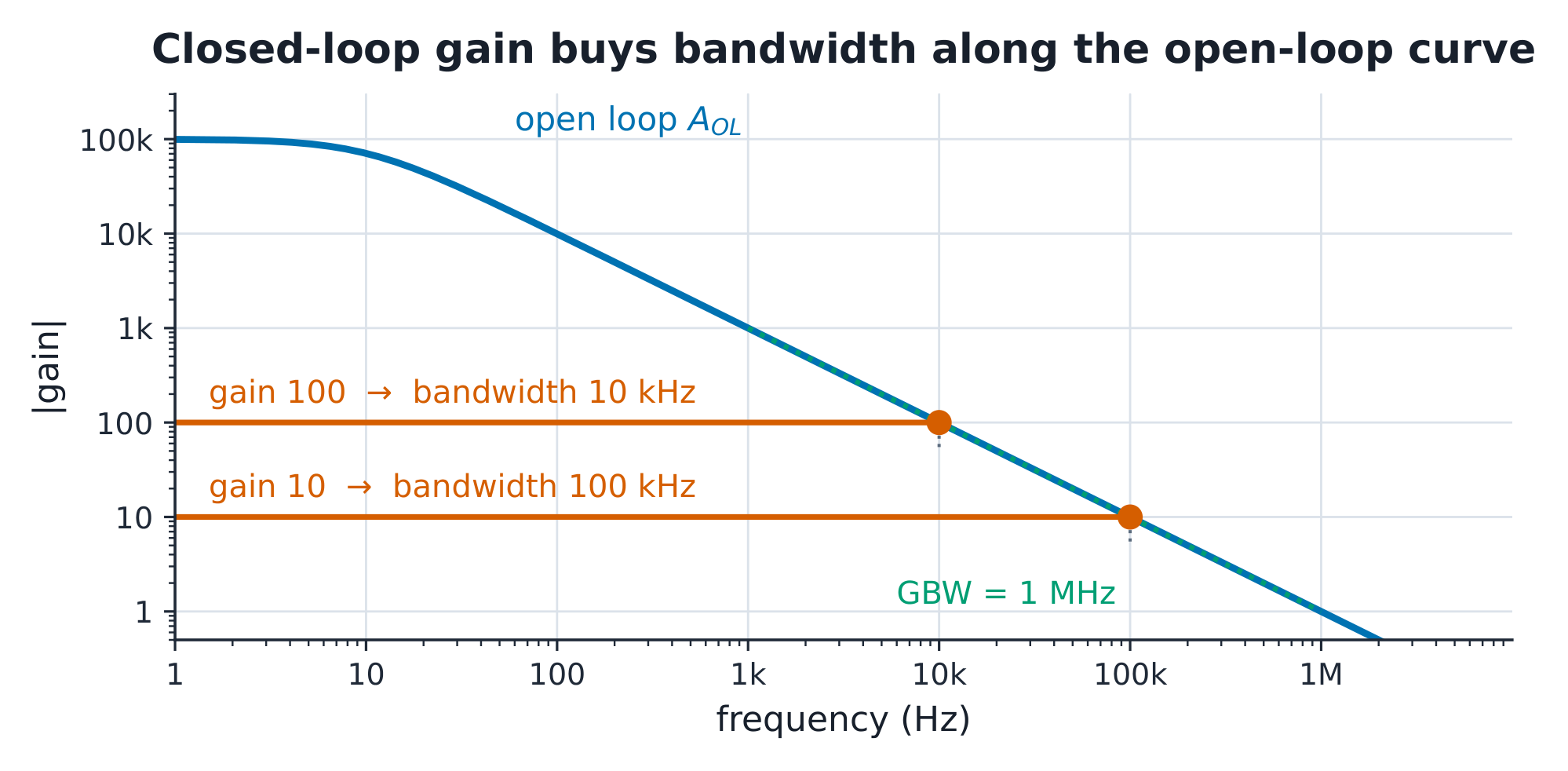
The gain-bandwidth hyperbola: closed-loop gain buys bandwidth along the open-loop curve
Worked example 1 (the four topologies and GBW). Inverting
$-R_f/R_{in}$ (input resistance $R_{in}$); non-inverting $1 + R_f/R_{in}$
(input resistance → ∞); transimpedance 跨阻放大器$v_o = -I_p R_f$
(photodiode: $2\ \mu\mathrm{A} \times 1\ \mathrm{M}\Omega = 2$ V);
summing $-(v_1 R_f/R_1 + v_2 R_f/R_2)$. An op-amp with gain-bandwidth
product 增益带宽积 GBW = 1 MHz at closed-loop 40 dB (100×) has bandwidth
10 kHz; at 20 dB (10×), 100 kHz ✓ (the product stays 1 MHz along the
hyperbola).
Worked example 2 (how wrong the golden rules are, escalated). The
$1/(1 + A_{OL}\beta_{fb})$ error factor, computed. Closed-loop gain 100
($\beta_{fb} = 0.01$): with $A_{OL} = 10^{5}$, $A_{CL} = 100/(1 + 1/1000) =
99.90$ — a 0.1% error, invisible on a scope. With a tired or high-frequency
op-amp where $A_{OL}$ has fallen to $10^{3}$ (remember unit 5.7: the
open-loop gain is already rolling off): $A_{CL} = 100/1.1 = 90.9$ — a 9.1%
error. So the golden rules are a loop-gain statement: where the loop gain
is large they are exact, and near the corner they quietly die. Check: at
10 kHz with GBW 1 MHz the open-loop gain has fallen to $10^{6}/10^{4} = 100$
— equal to the closed-loop gain, loop gain 1, and indeed that is the −3 dB
corner found in example 1.
Common mistakes. Using the inverting formula for a non-inverting stage
($1 + R_f/R_{in}$ differs by exactly 1 — at unity gain it is everything).
Forgetting the transimpedance stage's feedback resistor sets gain from
current, so the photodiode's capacitance still shapes the noise gain.
Summary: loop gain $A_{OL}\beta_{fb}$ is the truth meter for the golden
rules; error $= 1/(1 + A_{OL}\beta_{fb})$; GBW is a hyperbola — closed-loop
gain times bandwidth is conserved until the corner, where the rules die.
Every amplifier is a band-pass: coupling capacitors 耦合电容 set the low
corner $f_L = 1/(2\pi R_{eq}C)$ per stage ($R_{eq}$ = what the capacitor
sees, sources zeroed), and at the high end Miller capacitance 米勒电容
plus internal poles take over. The Miller derivation: a capacitor $C$ from
output to input of an inverting stage with gain $-A$ carries
$i = C\,d(v_{in} - v_o)/dt = C(1 + A)\,dv_{in}/dt$ — the input node behaves
as if it saw $C_M = C(1 + A)$ to ground. The dominant pole 主极点
approximation: one pole does most of the rolling,
$f_H \approx 1/(2\pi R_{eq}C_{eq})$.
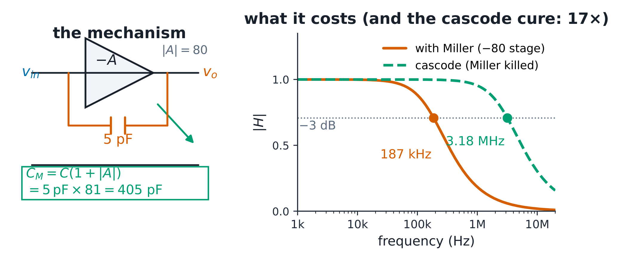
The Miller multiplication and the bandwidth it costs; the cascode reclaims 17×
Worked example 1 (the full band-pass, both corners). The unit-5.5 CE
stage: the coupling capacitor sees $R_{eq} = R_B \parallel r_\pi =
10.2\mathrm{k} \parallel 2.6\mathrm{k} = 2.08$ kΩ, so a 10 µF coupling gives
$f_L = 1/(2\pi \times 2.08\mathrm{k} \times 10\mu) = 7.7$ Hz. High end:
$C_{gb} = 5$ pF between base and collector where the stage gain is −80:
$C_M = 5\mathrm{p} \times 81 = 405$ pF, plus 20 pF of stray → $f_H =
1/(2\pi \times 2\mathrm{k} \times 425\mathrm{p}) = 187$ kHz. The stage passes
7.7 Hz to 187 kHz at gain −80. Checks: the coupling cap sees the parallel
combination (sources zeroed), not the sum — the classic $f_L$ slip; and the
−80 inside the Miller factor is the mid-band gain, already falling near
$f_H$ — the dominant-pole answer is optimistic by a few percent, the honest
reading.
Worked example 2 (the cascode and the cascade, escalated). A cascode
holds the collector nearly constant, killing the gain across the 5 pF:
$f_H = 1/(2\pi \times 2\mathrm{k} \times 25\mathrm{p}) = 3.18$ MHz — 17×
for one transistor: Miller explains the disease and the cure.
Cascade instead: two identical 187 kHz stages in series are each 3 dB down
there, so the pair is 6 dB down — the overall −3 dB point sits at
$187 \times \sqrt{2^{1/2} - 1} = 120$ kHz. A multistage amplifier pays for
its gain twice — once in Miller, once in cascade.
Common mistakes. Summing instead of paralleling resistances when finding
what the coupling capacitor sees; reporting the per-stage corner as the
system corner (the cascade shrinks it by $\sqrt{2^{1/n} - 1}$).
Summary: $f_L$ from coupling caps against zeroed-source resistance; Miller
multiplies by $(1 + |A|)$; the cascode removes it; cascades shrink corners
by $\sqrt{2^{1/n} - 1}$.
Explore
Miller moves the upper corner; cascades narrow both ends
$C_M=C(1+A),\quad f_H\approx\frac{1}{2\pi R C_{total}}$
Start with the worked gain magnitude 80, 5 pF feedback capacitor and 20 pF stray capacitance. Miller gives 425 pF in total and a high corner near 187 kHz. Suppress multiplication with the cascode idealisation to reach about 3.18 MHz. Then compare two buffered stages with one and probe the chain’s own half-power edge near 120 kHz. Changing the coupling capacitor moves the low corner independently.