| Enduring Understanding | Learning Objective | Essential Knowledge |
|---|---|---|
FUN-7 | FUN-7.A |
|
Differential Equations
AP Calculus AB · Topic 7
 5:24
Differential Equations
Many real situations are described not by a formula, but by a rate. A population grows faster when it is larger. A hot drink cools faster when it is hotter. An…
English narration · English + 中文 subtitles burned in
7.1
Modeling Situations with Differential Equations
Syllabus
Source: College Board AP Course and Exam Description
A nurse sets up a drip. The medicine flows into the blood at a steady rate, and the body removes it at a rate that grows with the amount already there. Nobody can write a formula for the amount $M(t)$ straight away, but everyone can say how fast it changes. That sentence is a differential equation, and this unit teaches you to write one, read its picture and solve it.
A differential equation 微分方程 is an equation that relates a function to its own derivatives 导数. It describes a situation by its rate of change 变化率. For example, "the rate of change of a quantity is proportional 成正比 to its size" becomes
$$\frac{dy}{dt} = ky.$$
Learning to translate a sentence about a rate into a differential equation is the first skill of this unit.
Worked example: from words to an equation. Read "is proportional to" as "equals a constant $k$ times", and "is inversely proportional to" as "equals a constant $k$ divided by".
| sentence | differential equation |
|---|---|
| A population $P$ grows at a rate proportional to its size. | $\dfrac{dP}{dt}=kP$ |
| The temperature $T$ of a drink changes at a rate proportional to the difference between $T$ and the room temperature $20^{\circ}$C. | $\dfrac{dT}{dt}=k(T-20)$ |
| The depth $h$ of water in a tank decreases at a rate proportional to $\sqrt h$. | $\dfrac{dh}{dt}=-k\sqrt h$, with $k>0$ |
| The volume $V$ changes at a rate inversely proportional to $V^2$. | $\dfrac{dV}{dt}=\dfrac{k}{V^2}$ |
The word "decreases" gives the minus sign; with it written explicitly, $k$ stays positive.
Explore
A rate equation's slope field
The equation $\tfrac{dy}{dt}=ky$ says the rate is proportional to $y$ — its slope field shows the growth it models.
Vocabulary
Train
| English |
|---|
| differential equation/ˌdɪfəˈrenʃl ɪˈkweɪʒn/ |
| derivative/dɪˈrɪvətɪv/ |
| rate of change/reɪt ɒv tʃeɪndʒ/ |
| proportional/prəˈpɔːʃənl/ |
7.2
Verifying Solutions for Differential Equations
Syllabus
| Enduring Understanding | Learning Objective | Essential Knowledge |
|---|---|---|
FUN-7 | FUN-7.B |
|
Source: College Board AP Course and Exam Description
A solution 解 of a differential equation is a function that makes it true. You can verify 验证 a proposed solution by differentiating it and substituting into the equation: if both sides match, it is a solution. Note a differential equation usually has infinitely many solutions – a whole family of solutions 解族 – indexed by an arbitrary constant 任意常数, which need not be an additive constant.
Worked example: verifying a family. Show that $y=Ce^{-x}+x-1$ is a solution of $\dfrac{dy}{dx}=x-y$ for every constant $C$.
Left side: $\dfrac{dy}{dx}=-Ce^{-x}+1$. Right side: $x-y=x-(Ce^{-x}+x-1)=1-Ce^{-x}$. The two sides are equal for all $x$, so every member of the family is a solution. (With $C=0$ the solution is the straight line $y=x-1$.)
Worked example: an unknown linear solution. For what values of $m$ and $b$ is the line $y=mx+b$ a solution of $\dfrac{dy}{dx}=2x-y$?
Substitute: the left side is $m$; the right side is $2x-(mx+b)=(2-m)x-b$. For $m=(2-m)x-b$ to hold for every $x$, the $x$-terms must match ($0=2-m$, so $m=2$) and the constants must match ($m=-b$, so $b=-2$). The solution is $y=2x-2$. Check: $\dfrac{dy}{dx}=2$ and $2x-(2x-2)=2$.
Common mistake. Substituting a single point and stopping. A solution must make the equation true at every $x$ in its domain, not at one point.
Explore
Solutions of dy/dx = ky
Each exponential $y=Ce^{kx}$ threads the slope field — verifying one just confirms its derivative matches $ky$.
Vocabulary
Train
| English |
|---|
| solution/səˈluːʃn/ |
| verify/ˈverɪfaɪ/ |
| family of solutions |
| arbitrary constant |
7.3
Sketching Slope Fields

Syllabus
| Enduring Understanding | Learning Objective | Essential Knowledge |
|---|---|---|
FUN-7 | FUN-7.C |
|
Source: College Board AP Course and Exam Description
A slope field 斜率场 draws the differential equation as a grid of short segments: at each point $(x,y)$ the segment has slope $\dfrac{dy}{dx}$ evaluated there. To sketch one, plug several points into the right-hand side and draw a small segment with that slope at each. The picture shows the shape of the solution curves 解曲线 without solving.
Exam skill. A common part gives a portion of a slope field and asks you to sketch the particular solution through a given point – start at the point and follow the segments, staying tangent 相切 to them.
Worked example. Sketch the slope field of $\dfrac{dy}{dx}=x-y$ at a few points. Substitute each point into $x-y$:
| point $(x,y)$ | $(0,0)$ | $(1,0)$ | $(0,1)$ | $(1,1)$ | $(2,1)$ | $(-1,1)$ |
|---|---|---|---|---|---|---|
| slope $x-y$ | $0$ | $1$ | $-1$ | $0$ | $1$ | $-2$ |
Draw a flat segment at $(0,0)$ and $(1,1)$, a segment rising at $45^{\circ}$ at $(1,0)$ and $(2,1)$, and so on. Every point on the line $y=x$ has slope $0$, and every point on $y=x-1$ has slope $1$.
Explore
Read a differential equation as a slope field
A slope field draws the slope $dy/dx$ at each point. A solution curve threads through, always tangent to the little segments — you can sketch it by following the flow.
Vocabulary
Train
| English |
|---|
| slope field/sləʊp fiːld/ |
| solution curve/səˈluːʃn kɜːv/ |
| tangent/ˈtændʒənt/ |
7.4
Reasoning Using Slope Fields

Syllabus
| Enduring Understanding | Learning Objective | Essential Knowledge |
|---|---|---|
FUN-7 | FUN-7.C |
|
Source: College Board AP Course and Exam Description
Solutions to a differential equation are functions or families of functions. Read a slope field to reason about behavior: where the segments are flat ($\tfrac{dy}{dx}=0$) the solution is momentarily level; where they steepen the solution rises or falls faster; equal slopes across every horizontal row suggest dependence only on $y$; equal slopes down every vertical column suggest dependence only on $x$.
Reading the field above. The right-hand side depends only on $M$, so every horizontal row of segments is identical. Where $M=40$ the slope is $0$ at every $t$, so the horizontal line $M=40$ is itself a solution: an equilibrium solution 平衡解. Below it $\dfrac{dM}{dt}>0$ (solutions rise towards 40); above it $\dfrac{dM}{dt}<0$ (solutions fall towards 40). A solution curve never crosses the equilibrium line; it only approaches it.
Concavity from the equation. Differentiate the differential equation itself, then substitute $\dfrac{dM}{dt}$ back in:
$$\frac{d^2M}{dt^2}=-\frac14\,\frac{dM}{dt}=-\frac14\cdot\frac14(40-M)=-\frac{1}{16}(40-M).$$
For $5\le M<40$ this is negative, so the solution through $(0,5)$ is concave down 下凹, as the picture shows.
Explore
Thread a curve through the field
A solution curve stays tangent to every dash it passes — drag the start point and watch it follow the field.
Vocabulary
Train
| English |
|---|
| equilibrium solution |
| concave down/kɒnˈkeɪv daʊn/ |
7.6
Finding General Solutions Using Separation of Variables
Syllabus
| Enduring Understanding | Learning Objective | Essential Knowledge |
|---|---|---|
FUN-7 | FUN-7.D |
|
Source: College Board AP Course and Exam Description
Many exam differential equations are solved by separation of variables 分离变量法. If $\dfrac{dy}{dx}$ factors into a function of $x$ times a function of $y$, move all $y$'s to one side and all $x$'s to the other, then integrate both sides where the divided factor is nonzero:
$$\frac{dy}{dx}=g(x)h(y)\;\Longrightarrow\;\int \frac{dy}{h(y)} = \int g(x)\,dx.$$
Add the constant of integration 积分常数 once (on the $x$-side). This gives the general solution 通解. Also check constant solutions 常数解 with $h(y)=0$ separately; division by $h(y)$ can lose them.
Worked example. Solve $\dfrac{dy}{dx}=xy$ with the initial condition $y(0)=2$. Separate and integrate:
$$\int\frac{dy}{y}=\int x\,dx\;\Rightarrow\;\ln|y|=\frac{x^2}{2}+C\;\Rightarrow\;y=Ae^{x^2/2}.$$
Applying $y(0)=2$ gives $A=2$, so the particular solution is $y=2e^{x^2/2}$.
Common mistakes. Adding the constant at the end: $y=e^{x^2/2}+C$ is wrong, because the constant enters when you integrate and becomes the multiplier $A=e^{C}$. Trying to separate an equation such as $\dfrac{dy}{dx}=x+y$: a sum cannot be written as $g(x)\,h(y)$.
Worked example: a power of $y$. Find the particular solution of $\dfrac{dy}{dx}=xy^2$ with $y(1)=1$, and state its domain.
$$\int y^{-2}\,dy=\int x\,dx\;\Rightarrow\;-\frac1y=\frac{x^2}{2}+C.$$
At $(1,1)$: $-1=\tfrac12+C$, so $C=-\tfrac32$. Then $-\dfrac1y=\dfrac{x^2-3}{2}$, so
$$y=\frac{2}{3-x^2}.$$
The formula breaks at $x=\pm\sqrt3$. The solution must live on one interval that contains the initial $x=1$, so its domain is $-\sqrt3<x<\sqrt3$.
Explore
The general solution is a family
Solving $\tfrac{dy}{dx}=ay$ gives $y=Ce^{ax}$ — one curve per constant, all fitting the same field.
Vocabulary
Train
| English |
|---|
| separation of variables/ˌsepəˈreɪʃn ɒv ˈveərɪəblz/ |
| constant of integration/ˈkɒnstənt ɒv ˌɪntɪˈɡreɪʃn/ |
| general solution/ˈdʒenərəl səˈluːʃn/ |
| constant solution |
7.7
Finding Particular Solutions Using Initial Conditions and Separation of Variables
Syllabus
| Enduring Understanding | Learning Objective | Essential Knowledge |
|---|---|---|
FUN-7 | FUN-7.E |
|
Source: College Board AP Course and Exam Description
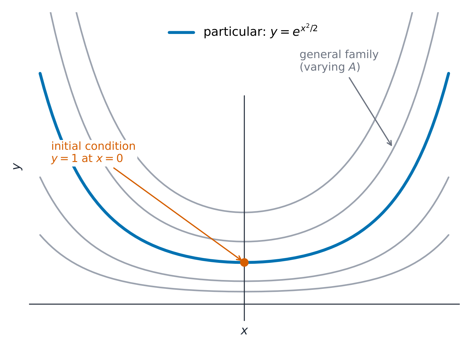
An initial condition 初始条件 – a known point $(x_0,y_0)$ – pins down one curve from the family. Substitute it to solve for the constant $C$; the result is the particular solution 特解. Uniqueness 唯一性 requires conditions: for $y'=F(x,y)$, continuity 连续性 of $F$ and its partial derivative 偏导数 with respect to $y$ near the initial point is a sufficient local condition. Watch for domain restrictions 定义域限制: keep the branch that contains the initial point (for example, the correct sign of a square root).
Worked example. Solve $\dfrac{dy}{dx}=\dfrac{x}{y}$ with $y(0)=-3$.
$$\int y\,dy=\int x\,dx \;\Rightarrow\; \frac{y^2}{2}=\frac{x^2}{2}+C.$$
Substitute $x=0$, $y=-3$ now, before solving for $y$: $\tfrac92=0+C$, so $C=\tfrac92$ and $y^2=x^2+9$. Taking the square root gives $y=\pm\sqrt{x^2+9}$; the initial value $y(0)=-3$ is negative, so the particular solution is
$$y=-\sqrt{x^2+9}.$$
Writing $y=+\sqrt{x^2+9}$ is the classic error: it fails the initial condition.
When there is no $y$ on the right. If $\dfrac{dy}{dx}=f(x)$ and $y(a)=y_0$, the Fundamental Theorem of Calculus gives the particular solution directly:
$$y(x)=y_0+\int_a^x f(t)\,dt.$$
This works even when $f$ has no antiderivative you can write down. For example, if $\dfrac{dy}{dx}=\sin(x^2)$ and $y(0)=4$, then $y(2)=4+\displaystyle\int_0^2\sin(t^2)\,dt\approx 4+0.805=4.805$ (calculator).
Explore
The initial point picks one curve
The general solution is a whole family; the initial condition $y(x_0)=y_0$ selects the single curve through that point.
Vocabulary
Train
| English |
|---|
| initial condition/ɪˈnɪʃl kənˈdɪʃn/ |
| particular solution/pəˈtɪkjʊlə səˈluːʃn/ |
| uniqueness |
| continuity/kɒntɪˈnjuːɪti/ |
| partial derivative |
| domain restriction/dəˈmeɪn rɪˈstrɪkʃn/ |
7.8
Exponential Models with Differential Equations
Syllabus
| Enduring Understanding | Learning Objective | Essential Knowledge |
|---|---|---|
FUN-7 | FUN-7.F |
|
FUN-7.G |
|
Source: College Board AP Course and Exam Description
The most important model is exponential growth and decay 指数增长与衰减. The equation $\dfrac{dy}{dt}=ky$ (rate proportional to size) has the solution:
$$y = y_0\,e^{kt},$$
where $y_0$ is the value at $t=0$. Here $k>0$ gives growth and $k<0$ gives decay. You can derive this by separation of variables ($\int \tfrac{dy}{y} = \int k\,dt$), and it models processes like population growth and radioactive decay 放射性衰变. In Newton's law of cooling 牛顿冷却定律 with fixed ambient temperature, apply this exponential model to the temperature difference from the surroundings. A follow-up part may ask for $\dfrac{d^2y}{dt^2}$: differentiate $\dfrac{dy}{dt}=ky$ again (using $\dfrac{dy}{dt}=ky$) to express it in terms of $y$.
Worked example. A sample decays by $\dfrac{dy}{dt}=-0.10\,y$ (in years) from $y_0=50\ \text{g}$. The solution is $y=50e^{-0.10t}$, so after $10$ years $y=50e^{-1}=18.4\ \text{g}$. Its half-life 半衰期 solves $25=50e^{-0.10t}$, i.e. $e^{-0.10t}=\tfrac12$, giving $t=\dfrac{\ln 2}{0.10}=6.9\ \text{years}$ – independent of the starting amount.
Worked example: Newton's law of cooling. Coffee at $90^{\circ}$C is left in a room at $20^{\circ}$C. Its temperature $T$ obeys $\dfrac{dT}{dt}=-k\,(T-20)$, with $t$ in minutes. After $5$ minutes it is $70^{\circ}$C. When does it reach $40^{\circ}$C?
The temperature difference $D=T-20$ decays exponentially: $D=70e^{-kt}$ (the start value is $90-20=70$), so
$$T=20+70e^{-kt}.$$
Use $T(5)=70$: $50=70e^{-5k}$, so $k=\dfrac{\ln(7/5)}{5}\approx 0.0673$ per minute. For $T=40$:
$$20=70e^{-kt} \;\Rightarrow\; t=\frac{\ln 3.5}{k}\approx\frac{1.2528}{0.06729}\approx 18.6 \text{ minutes}.$$
Common error: writing $T=90e^{-kt}$, which would cool the coffee towards $0^{\circ}$C instead of towards room temperature.

Worked example: limited growth. Medicine enters the blood so that the amount $M$, in milligrams, satisfies $\dfrac{dM}{dt}=\tfrac14(40-M)$, with $t$ in hours and $M(0)=5$.
(a) Solve. Separate: $\displaystyle\int\frac{dM}{40-M}=\int\frac14\,dt$, so $-\ln|40-M|=\dfrac t4+C$. At $t=0$: $-\ln 35=C$. Since $M<40$, $|40-M|=40-M$, and
$$40-M=35e^{-t/4}\;\Rightarrow\;M=40-35e^{-t/4}.$$
(b) Long-run behaviour. As $t\to\infty$, $e^{-t/4}\to0$, so $\displaystyle\lim_{t\to\infty}M(t)=40$. In context: over a long time the amount of medicine in the blood approaches $40$ milligrams. Always give the units and the context.
(c) Tangent-line estimate. $M'(0)=\tfrac14(40-5)=8.75$, so the linear approximation 线性近似 at $t=0$ gives $M(2)\approx5+8.75\cdot2=22.5$ mg. Is this too big or too small? From the slope field section, $\dfrac{d^2M}{dt^2}=-\tfrac1{16}(40-M)<0$, so the graph is concave down and lies below its tangent line: the estimate is an overestimate 高估. (Check: $M(2)=40-35e^{-0.5}\approx18.8$ mg.)
The pattern $\dfrac{dy}{dt}=k(L-y)$ always gives $y=L-(L-y_0)e^{-kt}$: the gap $L-y$ decays exponentially, exactly like Newton's law of cooling.
Explore
An exponential growth/decay model
y = a·e^(bx) + c
The equation $dy/dt=ky$ has exponential solutions: quantity changes at a rate proportional to itself, giving unbounded growth ($k>0$) or decay to zero ($k<0$).
Vocabulary
Train
| English |
|---|
| exponential growth and decay/ˌekspəˈnenʃl ɡrəʊθ ænd dɪˈkeɪ/ |
| radioactive decay/ˌreɪdɪəʊˈæktɪv dɪˈkeɪ/ |
| Newton's law of cooling |
| half-life/hɑːf laɪf/ |
| linear approximation/ˈlɪnɪə əˌprɒksɪˈmeɪʃn/ |
| overestimate/ˌəʊvəˈrestɪmət/ |
7.8
Exam tips
- Solve a separable equation by getting all $y$ on one side and all $x$ on the other, then integrating both sides (add $+C$ once).
- Use the initial condition to find $C$ (a particular solution).
- Sketch or read a slope field: the little segments show $\tfrac{dy}{dx}$ at each point, and a solution curve follows them.
- Recognise exponential models $\tfrac{dy}{dt}=ky\Rightarrow y=Ce^{kt}$ (growth/decay).
- A differential equation gives the slope — you must integrate to recover the function.
Practice.
- Write a differential equation: the rate at which a rumour spreads in a school of $1000$ students is proportional to the product of the number $N$ who have heard it and the number who have not.
- Verify that $y=3e^{2x}-1$ is a solution of $\dfrac{dy}{dx}=2y+2$.
- For $\dfrac{dy}{dx}=y-x$, find the slope of the segment at $(2,5)$, and describe every point where the segments are horizontal.
- Find the particular solution of $\dfrac{dy}{dx}=\dfrac{x^2}{y}$ with $y(0)=-2$.
- The amount $A$ of salt, in grams, in a tank satisfies $\dfrac{dA}{dt}=\dfrac{12-A}{3}$ with $A(0)=0$, $t$ in minutes. Find $A(t)$ and $\displaystyle\lim_{t\to\infty}A(t)$, and interpret the limit.
- $\dfrac{dy}{dt}=0.5(y-10)$ with $y(0)=4$. Find $\dfrac{d^2y}{dt^2}$ in terms of $y$, use the tangent line at $t=0$ to estimate $y(1)$, and decide whether the estimate is too big or too small.
Answers.
- $\dfrac{dN}{dt}=kN(1000-N)$.
- $\dfrac{dy}{dx}=6e^{2x}$ and $2y+2=6e^{2x}-2+2=6e^{2x}$; the sides agree for all $x$.
- Slope $5-2=3$. Horizontal where $y-x=0$: every point on the line $y=x$.
- $\dfrac{y^2}{2}=\dfrac{x^3}{3}+C$; at $(0,-2)$, $C=2$, so $y^2=\dfrac{2x^3}{3}+4$. Since $y(0)<0$, $y=-\sqrt{\dfrac{2x^3}{3}+4}$, for $x>-\sqrt[3]{6}$.
- $A=12-12e^{-t/3}$; the limit is $12$: over a long time the tank holds close to $12$ grams of salt.
- $\dfrac{d^2y}{dt^2}=0.5\dfrac{dy}{dt}=0.25(y-10)$. $y'(0)=-3$, so $y(1)\approx4-3=1$. For $y<10$, $\dfrac{d^2y}{dt^2}<0$: concave down, so the estimate is too big (exact: $10-6e^{0.5}\approx0.11$).
Interactive lessons on this topic
Work through it step by step, with instant-check exercises.
- Modeling Situations with Differential Equations
- Verifying Solutions for Differential Equations
- Sketching Slope Fields
- Reasoning Using Slope Fields
- Finding General Solutions Using Separation of Variables
- Finding Particular Solutions Using Initial Conditions and Separation of Variables
- Exponential Models with Differential Equations