Skip to content · ⁨דלג לתוכן⁩

Probability & Statistics 1 · ⁨הסתברות וסטטיסטיקה 1⁩

A-Level Mathematics · ⁨מתמטיקה A-Level⁩ · Topic 5 · ⁨נושא 5⁩

Video lesson for this topic · ⁨שיעור וידאו לנושא זה⁩ Open the video page · ⁨פתח את עמוד הוידאו⁩
11:38

הסתברות וסטטיסטיקה 1

השלכת קובייה אחת, והתוצאה היא משהו שאין לנבא. אך השלכו אותה אלפי פעמים, או מדדו את הגובה של אלפי אנשים, ומשהו מדהים…

English narration · English + 中文 subtitles burned in · ⁨קריאת קול באנגלית · תרגום אנגלי + סינית שרוף בתוך הסרטון⁩

English

This handout covers Topic 5: Probability & Statistics 概率统计 1. It is about describing data, counting choices, and working out the chance of events.

עברית

חוברת זו מכסה נושא 5: הסתברות וסטטיסטיקה 1. מדובר בתיאור נתונים, ספירת אפשרויות וחילוף ההסתברות לאירועים.

5.1

Representation of data · ⁨היצגות נתונים⁩

Syllabus · ⁨סיילבוס⁩
English
Candidates should be able to: Notes and examples
• select a suitable way of presenting raw statistical data, and discuss advantages and/or disadvantages that particular representations may have
• draw and interpret stem-and-leaf diagrams, box-and-whisker plots, histograms and cumulative frequency graphs Including back-to-back stem-and-leaf diagrams.
• understand and use different measures of central tendency (mean, median, mode) and variation (range, interquartile range, standard deviation) e.g. in comparing and contrasting sets of data.
• use a cumulative frequency graph e.g. to estimate medians, quartiles, percentiles, the proportion of a distribution above (or below) a given value, or between two values.
• calculate and use the mean and standard deviation of a set of data (including grouped data) either from the data itself or from given totals $\Sigma x$ and $\Sigma x^2$, or coded totals $\Sigma(x - a)$ and $\Sigma(x - a)^2$, and use such totals in solving problems which may involve up to two data sets.
עברית
המועמדים אמורים להיות מסוגלים: הערות לדוגמאות
• לבחור בדרך מתאימה להצגת נתונים סטטיסטיים ראשוניים, לדון יתרונות ו/או חסרונות שמייצוגים מסוימים עשויים להיות להם
• לצייר ול解读 דיאגרמות עמוד-עלים, תרשימי קופסה-שפך, היסטוגרמות וגרפי תדירות מצטברת כולל דיאגרמות עמוד-עלים הפוכות.
• להבין ולהשתמש במדדים שונים של מרכזיות (ממוצע, חציון, מוֹד) וDispersion (מרווח, טווח רבעוני, סטיית תקן) לדוגמה: בהשוואה ובניגוד בין קבוצות נתונים.
• להשתמש בגרף תדירות מצטברת לדוגמה: כדי להעריך חציונים, רבעונים, אחוזונים, את המ proportion של ההתפלגות מעל (או מתחת) לערך נתון, או בין שני ערכים.
• לחשב ולהשתמש בממוצע ובסטיית התקן של קבוצת נתונים (כולל נתונים קבוצתיים) גם מהנתונים עצמם וגם ממספרים הנתונים $\Sigma x$ ו$\Sigma x^2$, או ממספרים קודדים $\Sigma(x - a)$ ו$\Sigma(x - a)^2$, ולהשתמש במספרים אלו בפתרון בעיות שיכללו עד שתי קבוצות נתונים.

Source: Cambridge International syllabus · ⁨מקור: הסיילבוס הבינלאומי של קמבריד'ג'⁩

English

Choose a diagram that suits the data. You should be able to draw and read:

  • a stem-and-leaf diagram 茎叶图 (keeps the original values and shows the shape); two data sets are compared with a back-to-back 背靠背 version – a shared central stem, one set's leaves increasing to the left and the other's to the right, so you can compare their medians and spreads at a glance;
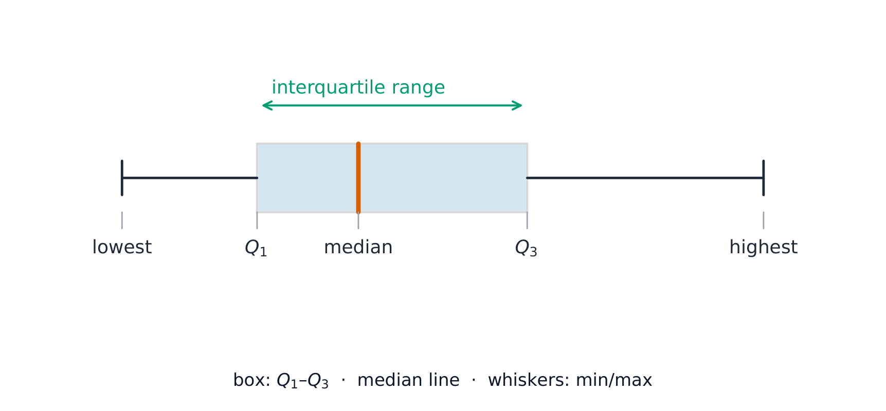
  • a box-and-whisker plot 箱线图 (shows the lowest value, the three quartiles, and the highest value);
  • a histogram 直方图 (for grouped data, where the area of each bar shows the frequency);
  • a cumulative frequency 累积频数 graph (running totals, used to estimate the median and quartiles).

Averages and spread

A measure of central tendency 集中趋势 is a single "middle" value:

  • the mean 平均数 $\bar{x} = \dfrac{\sum x}{n}$ (the average);
  • the median 中位数 (the middle value when the data is in order);
  • the mode 众数 (the most common value).

A measure of variation 离散程度 shows how spread out the data is:

  • the range (of data) 极差 (highest $-$ lowest);
  • the interquartile range 四分位距 (upper quartile $-$ lower quartile);
  • the standard deviation 标准差 $\sigma = \sqrt{\dfrac{\sum x^2}{n} - \bar{x}^2}$.

You often work from the totals $\sum x$ and $\sum x^2$. The square of the standard deviation is the variance 方差.

Worked example. For $10$ values, $\sum x = 50$ and $\sum x^2 = 300$. Find the mean and standard deviation.

$$\bar{x} = \frac{50}{10} = 5, \qquad \sigma = \sqrt{\frac{300}{10} - 5^2} = \sqrt{30 - 25} = \sqrt{5} = 2.24.$$

Coding 编码 makes big numbers easier. Replace each value by $t=x-a$ for a convenient assumed mean 假定平均数 $a$. Then $\bar{x}=a+\bar{t}$, while the standard deviation is unchanged (shifting every value does not spread the data). So from the coded totals $\sum(x-a)$ and $\sum(x-a)^2$ you get $\bar x$ and $\sigma$ directly, and two data sets can be compared through their coded totals.

עברית

בחרו גרף המתאים לנתונים. עליכם להיות מסוגלים לצייר ולקרוא:

  • גרף עמוד-עלים (שומר על הערכים המקוריים ומראה את הצורה); שני קבוצות נתונים משווים עם גרף דו-צדדי – עמוד מרכזי משותף, עלי קבוצה אחת גדלים שמאלה ועלי הקבוצה השנייה ימינה, כך שתוכלו להשוות בין המדiane שלהם והתפוצה במבט ראשון;
  • תרשים קופסה וזנבות (מראה את הערך הנמוך ביותר, שלושת הרבעונים והערך הגבוה ביותר);
  • היסטוגרמה (לנתונים מקבוצות, כאשר השטח של כל עמודה מייצג את התדירות);
  • גרף תדירות מצטברת (סיכומים רציפים, משמש להערכת המדiane ורבעונים).
עקומת תדירות מצטברת בצורת S עם קווים מקווקים לקריאת המדiane בחצי התדירות הכוללת
עקומת תדירות מצטברת היא בצורת S; לקרוא את הממוצע החצי (המיון) באופן אופקי מול חצי התדירות הכוללת, ואת הרבעונים מתוך רביע ראשון ושלישי.
תרשים קופסאות-זנבות עם זנבות לערכים הנמוכים והגבוהים ביותר וקופסה של רבעונים
הקופסה משתרעת בין הרבעונים $Q_1$ ל$Q_3$; הזנבות מגיעים לערכים הנמוכים והגבוהים ביותר.

ממוצעים פיזור

מדד מיקוד הוא ערך "אמצעי" יחיד:

  • הממוצע $\bar{x} = \dfrac{\sum x}{n}$ (הממונה);
  • המיון (הערך האמצעי כאשר הנתונים מסודרים);
  • המודוס (הערך הנפוץ ביותר).

מדד בדידות מראה עד כמה הנתונים מפוזרים:

  • הטווח (של נתונים) (הגבוה $-$ הנמוך);
  • הטווח הרבעוני (רבעון עליון $-$ רבעון תחתון);
  • סטיית התקן $\sigma = \sqrt{\dfrac{\sum x^2}{n} - \bar{x}^2}$.

לעיתים קרובות עובדים מהסכומים $\sum x$ ו$\sum x^2$. ריבוע סטיית התקן הוא שונות.

דוגמה פותרת. עבור $10$ ערכים, $\sum x = 50$ ו$\sum x^2 = 300$. מצאו את הממוצע ואת סטיית התקן.

$$\bar{x} = \frac{50}{10} = 5, \qquad \sigma = \sqrt{\frac{300}{10} - 5^2} = \sqrt{30 - 25} = \sqrt{5} = 2.24.$$

קוד מקל על עבודה עם מספרים גדולים. החליפו כל ערך ב$t=x-a$ כדי לקבל ממוצע משוער נוח $a$. אזי $\bar{x}=a+\bar{t}$, בעוד שסטיית התקן נשארת לא משתנה (הזזת כל הערכים אינה מפזרת את הנתונים). לכן מהסכומים המקודדים $\sum(x-a)$ ו$\sum(x-a)^2$ תקבלו $\bar x$ ו$\sigma$ ישירות, וניתן להשוות בין שני קבוצות נתונים דרך הסכומים המקודדים שלהן.

Explore · ⁨חקור⁩

Spread and the bell · ⁨פיזור והפעמון⁩

P(−k < Z < k)

Spread is measured in standard deviations — about 68% of data lies within 1 sd, 95% within 2. · ⁨פיזור נמדד ב-סטייות תקן — כ-68% מהנתונים נמצאים בתוך 1 sd, וכ-95% בתוך 2.⁩

Vocabulary · ⁨מילון מונחים⁩ Train · ⁨אימון⁩
English עברית
stem-and-leaf diagram/stem ænd liːf ˈdaɪəɡræm/ תרשים עלים וענפים
back-to-back/bæk tə bæk/ גבול-לגבול
box-and-whisker plot/bɒks ænd ˈwɪskə plɒt/ תרשים קופסה וזנבות
histogram/ˈhɪstəɡræm/ היסטוגרמה
cumulative frequency/ˈkjuːmjʊlətɪv ˈfriːkwənsi/ תדירות מצטברת
measure of central tendency/ˈmeʒə ɒv ˈsentrəl ˈtendənsi/ מדד מיקום מרכזי
mean/miːn/ ממוצע
median/ˈmiːdiːən/ חציון
mode/məʊd/ מודוס (תדירות השכיחה ביותר)
variation/ˌveərɪˈeɪʃn/ וריאות
5.2

Permutations and combinations · ⁨פרמוטציות וקומבינציות⁩

Syllabus · ⁨סיילבוס⁩
English
Candidates should be able to: Notes and examples
• understand the terms permutation and combination, and solve simple problems involving selections
• solve problems about arrangements of objects in a line, including those involving – repetition (e.g. the number of ways of arranging the letters of the word ‘NEEDLESS’) – restriction (e.g. the number of ways several people can stand in a line if two particular people must, or must not, stand next to each other). Questions may include cases such as people sitting in two (or more) rows. Questions about objects arranged in a circle will not be included.
עברית
המועמדים אמורים להיות מסוגלים: הערות לדוגמאות
• הבנת המונחים פרמוטציה וקומבינציה, פתרון בעיות פשוטות הקשורות לבחירות
• פתרון בעיות הקשורות לסידור אובייקטים בשורה, כולל אלו העוסקות ב– חזרה (למשל, מספר הדרכים לסדר אותיות במילה ‘NEEDLESS’) – הגבלה (למשל, מספר הדרכים מספר אנשים יכולים לעמוד בשורה אם שניים מסוימים חייבים או אסור להם לעמוד זה לצד זה). ייתכן שהשאלות יכללו מקרים כמו אנשים היושבים בשתי (או יותר) שורות. שאלות הקשורות לאובייקטים מסודרים במעגל לא יכללו.

Source: Cambridge International syllabus · ⁨מקור: הסיילבוס הבינלאומי של קמבריד'ג'⁩

English

A permutation 排列 is an arrangement where order matters; a combination 组合 is a selection where order does not matter. The numbers are

$${}^nP_r = \frac{n!}{(n-r)!}, \qquad {}^nC_r = \binom{n}{r} = \frac{n!}{r!\,(n-r)!}.$$
To arrange objects in a line when some are repeated, divide by the factorial of each repeat count.

Worked example. How many different arrangements are there of the letters of the word NEEDLESS?

There are $8$ letters, with E repeated $3$ times and S repeated $2$ times:

$$\frac{8!}{3!\,2!} = \frac{40320}{6 \times 2} = 3360.$$

עברית

פרמוטציה היא סידור בו הסדר חשוב; קומבינציה היא בחירה בה הסדר אינו חשוב. המספרים הם

$${}^nP_r = \frac{n!}{(n-r)!}, \qquad {}^nC_r = \binom{n}{r} = \frac{n!}{r!\,(n-r)!}.$$
לסדר חפצים בשורה כאשר חלקם חוזרים, יש לחלק בפאקטוריאל של מספר החזרות בכל קבוצה.

פרמוטציה: הסדר חשוב (AB ≠ BA). קומבינציה: הסדר אינו חשוב ({A,B} = {B,A})
הסדר חשוב בהפרעה, אך לא בקומבינציה

דוגמה פותרת. כמה סידורים שונים יש של אותיות המילה NEEDLESS?

יש $8$ אותיות, כאשר E מופיעה $3$ פעמים ו-S מופיעה $2$ פעמים:

$$\frac{8!}{3!\,2!} = \frac{40320}{6 \times 2} = 3360.$$

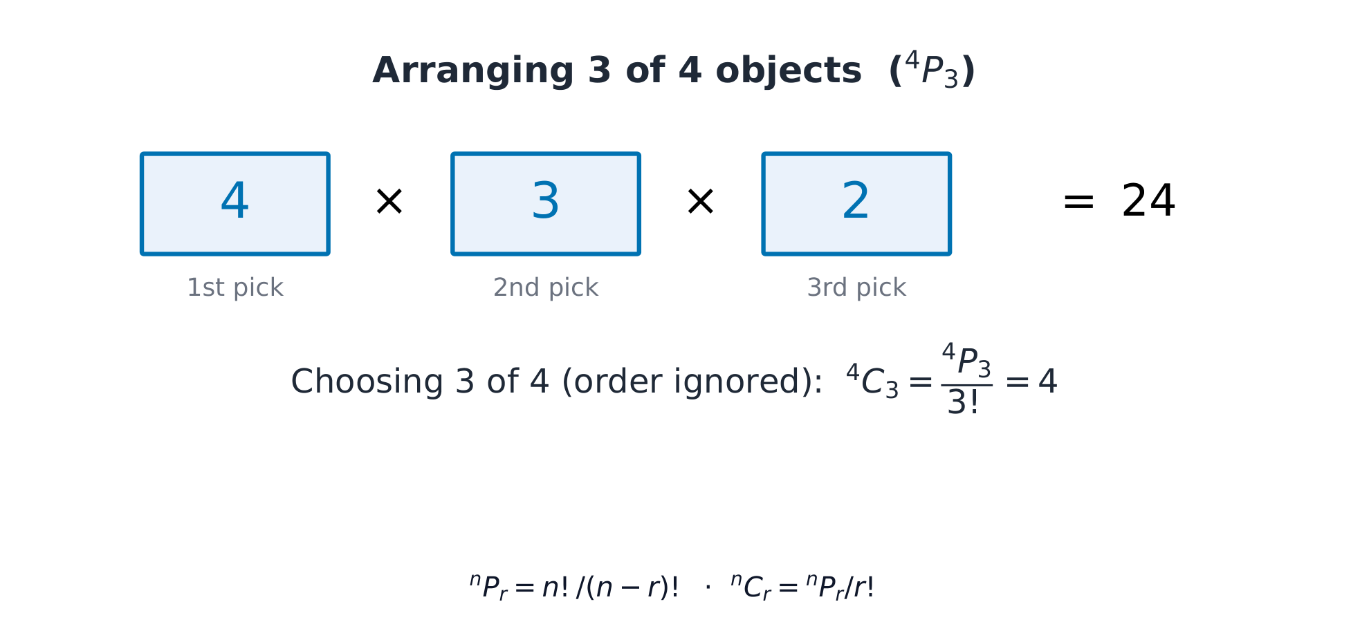
סידור 3 מתוך 4 אובייקטים: 4×3×2 = 24 = ⁴P₃; קומבינציות מחלקות ב-r!
nPr = n!/(n−r)!; nCr = nPr/r!
Explore · ⁨חקור⁩

Permutation or combination lab · ⁨מעבדה לפרמוטציה או קומבינציה⁩

Choose whether order matters in a counting problem. · ⁨בחר האם סדר חשוב במשהו ספירה.⁩

Vocabulary · ⁨מילון מונחים⁩ Train · ⁨אימון⁩
English עברית
range (of data)/reɪndʒ/ תחום (של נתונים)
interquartile range/ˌɪntəˈkwɔːtaɪl reɪndʒ/ טווח רביעי
standard deviation/ˈstændəd ˌdiːvɪˈeɪʃn/ סטיית תקן
variance/ˈveərɪəns/ סטייה
Coding/ˈkəʊdɪŋ/ קידוד
assumed mean/əˈsjuːmd miːn/ ממוצע משוער
permutation/ˌpɜːmjuːˈteɪʃn/ פרימותציה
combination/ˌkɒmbɪˈneɪʃn/ קבוצות (קומבינציה)
mutually exclusive events/ˈmjuːtʃuːəli eksˈkluːsɪv ɪˈvents/ אירועים בלתי תואמים
independent events/ˌɪndɪˈpendənt ɪˈvents/ אירועים בלתי תלויים
conditional probability/kənˈdɪʃənl ˌprɒbəˈbɪlɪti/ הסתברות מותנית
discrete random variable/dɪˈskriːt ˈrændəm ˈveərɪəbl/ משתנה אקראי בדיד
probability distribution table/ˌprɒbəˈbɪlɪti ˌdɪstrɪˈbjuːʃn ˈteɪbl/ טבלת התפלגות הסתברות
expectation/ekspɪkˈteɪʃn/ צפוי (תוחלת)
binomial distribution/baɪˈnəʊmɪəl ˌdɪstrɪˈbjuːʃn/ חלוקה בינומית
geometric distribution/ˌdʒiːəʊˈmetrɪk ˌdɪstrɪˈbjuːʃn/ התפלגות גיאומטרית
5.3

Probability · ⁨הסתברות⁩

Syllabus · ⁨סיילבוס⁩
English
Candidates should be able to: Notes and examples
evaluate probabilities in simple cases by means of enumeration of equiprobable elementary events, or by calculation using permutations or combinations e.g. the total score when two fair dice are thrown. e.g. drawing balls at random from a bag containing balls of different colours.
use addition and multiplication of probabilities, as appropriate, in simple cases Explicit use of the general formula $\text{P}(A \cup B) = \text{P}(A) + \text{P}(B) - \text{P}(A \cap B)$ is not required.
understand the meaning of exclusive and independent events, including determination of whether events $A$ and $B$ are independent by comparing the values of $\text{P}(A \cap B)$ and $\text{P}(A) \times \text{P}(B)$
calculate and use conditional probabilities in simple cases. e.g. situations that can be represented by a sample space of equiprobable elementary events, or a tree diagram. The use of $\text{P}(A|B) = \frac{\text{P}(A \cap B)}{\text{P}(B)}$ may be required in simple cases.
עברית
המועמדים אמורים להיות מסוגלים: הערות לדוגמאות
הערכת סיכויים במקרים פשוטים באמצעות ספירה של אירועים יסודיים שוווי-סיכוי, או חישוב באמצעות פרמוטציות או קומבינציות לדוגמה: סך הנקודות כאשר משליכים שני קוביות הוגנות. לדוגמה: גרירת כדורים באופן אקראי מתוך תיק המכיל כדורים בצבעים שונים.
שימוש בחיבור ובכפל סיכויים, בהתאם, במקרים פשוטים שימוש מפורש בנוסחה הכללית $\text{P}(A \cup B) = \text{P}(A) + \text{P}(B) - \text{P}(A \cap B)$ אינו נדרש.
הבנת המשמעות של אירועים בדידים ובלתי תלויים, כולל קביעה האם אירועים $A$ ו$B$ הם בלתי תלויים על ידי השוואת הערכים של $\text{P}(A \cap B)$ ו$\text{P}(A) \times \text{P}(B)$
חישוב והשתמש בסיכויים תנאי במקרים פשוטים. לדוגמה: מצבים שיכולים להיות מיוצגים על ידי מרחב דגימה של אירועים יסודיים שוווי-סיכוי, או על ידי דיאגרמת עץ. שימוש ב$\text{P}(A|B) = \frac{\text{P}(A \cap B)}{\text{P}(B)}$ עשוי להיות נדרש במקרים פשוטים.

Source: Cambridge International syllabus · ⁨מקור: הסיילבוס הבינלאומי של קמבריד'ג'⁩

English

Find a probability by counting equally likely outcomes, or by using permutations and combinations. Combine probabilities with these rules:

  • addition for "or": $P(A \cup B) = P(A) + P(B) - P(A \cap B)$;
  • multiplication for "and" when events are independent: $P(A \cap B) = P(A)\,P(B)$.

Two events are mutually exclusive events 互斥事件 if they cannot both happen, and independent events 独立事件 if one happening does not change the chance of the other. To test independence, check whether $P(A \cap B) = P(A)\times P(B)$. A conditional probability 条件概率 is the chance of $A$ given that $B$ has happened: $P(A \mid B) = \dfrac{P(A \cap B)}{P(B)}$.

Worked example. Events have $P(A) = 0.5$, $P(B) = 0.4$ and $P(A \cap B) = 0.2$. Are $A$ and $B$ independent?

Test: $P(A)\times P(B) = 0.5 \times 0.4 = 0.2 = P(A \cap B)$. The values are equal, so $A$ and $B$ are independent.

עברית
מגוון קוביות דייס רב-פנים
גרעש: נקודת התחלה מוכרת להסתברות.

מצאו הסתברות על ידי ספירת תוצאות שוות-סיכוי, או על ידי שימוש בהפרעות ובקומבינציות. שילבו הסתברויות עם הכללים הבאים:

  • חיבור עבור "או": $P(A \cup B) = P(A) + P(B) - P(A \cap B)$;
  • כפל עבור "וגם" כאשר האירועים עצמאיים: $P(A \cap B) = P(A)\,P(B)$.
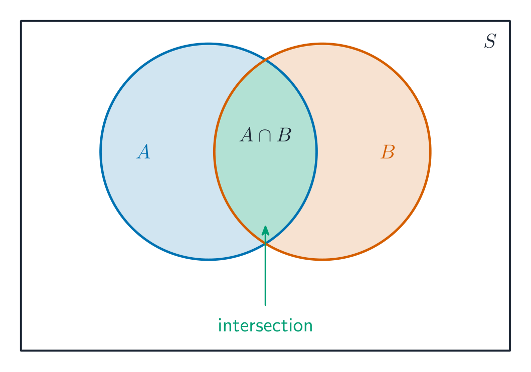
מעגלים חופפים בתוך מלבן, כאשר החפיפה צלולה כחיתוך
החפיפה של שני המעגלים היא $A\cap B$; כלל החיבור חוסר אותה פעם אחת כדי שלא תיספר פעמיים.

שני אירועים הם אירועים בלתי תואמים אם לא יכול לקרות גם אחד וגם השני, ואירועים עצמאיים אם קרה אחד מהם אינו משנה את הסיכוי לשני. לבדוק עצמאות, בדקו האם $P(A \cap B) = P(A)\times P(B)$. הסתברות מותנית היא הסיכוי ל$A$ נתון שה$B$ קרה: $P(A \mid B) = \dfrac{P(A \cap B)}{P(B)}$.

דוגמה מפורטת. לאירועים יש $P(A) = 0.5$, $P(B) = 0.4$ ו$P(A \cap B) = 0.2$. האם $A$ ו$B$ עצמאיים?

בדיקה: $P(A)\times P(B) = 0.5 \times 0.4 = 0.2 = P(A \cap B)$. הערכים שווים, ולכן $A$ ו$B$ עצמאיים.

Explore · ⁨חקור⁩

Conditional probability · ⁨הסתברות מותנית⁩

Change the probabilities and read the tree. This is how P(A and B) and conditional probability fit together. · ⁨שנה את ההסתברותות וקרא את העץ. כך P(A and B) והסתברות תנאיית משלימים זה את זה.⁩

Watch lesson · ⁨צפה בשיעור⁩
5.4

Discrete random variables · ⁨משתנים מקריים דיסקרטיים⁩

Syllabus · ⁨סיילבוס⁩
English
Candidates should be able to: Notes and examples
draw up a probability distribution table relating to a given situation involving a discrete random variable $X$, and calculate $\text{E}(X)$ and $\text{Var}(X)$
use formulae for probabilities for the binomial and geometric distributions, and recognise practical situations where these distributions are suitable models Including the notations $\text{B}(n, p)$ and $\text{Geo}(p)$. $\text{Geo}(p)$ denotes the distribution in which $p_r = p(1 - p)^{r-1}$ for $r = 1, 2, 3, \dots$.
use formulae for the expectation and variance of the binomial distribution and for the expectation of the geometric distribution. Proofs of formulae are not required.
עברית
המועמדים אמורים להיות מסוגלים: הערות לדוגמאות
הרכבת טבלת חלוקת סיכויים הקשורה למצב נתון המעורב במשתנה אקראי בדיד $X$, וחישוב $\text{E}(X)$ ו$\text{Var}(X)$
להשתמש בנוסחאות להסתברויות עבור החלוקות בינומית וגיאומטרית, ולזהות מצבים פרקטיים בהם חלוקות אלו מהוות מודלים מתאימים כולל סימנויות $\text{B}(n, p)$ ו$\text{Geo}(p)$. $\text{Geo}(p)$ מייצג את החלוקה שבה $p_r = p(1 - p)^{r-1}$ עבור $r = 1, 2, 3, \dots$.
שימוש בנוסחאות עבור התצופה (הצפייה) והשונות של החלוקה הדו-תוצאתית ועבור התצופה של החלוקה הגיאומטרית. הוכחות לנוסחאות אינן נדרשות.

Source: Cambridge International syllabus · ⁨מקור: הסיילבוס הבינלאומי של קמבריד'ג'⁩

English

A discrete random variable 离散型随机变量 $X$ takes separate values, each with a probability. List them in a probability distribution table 概率分布表; the probabilities must add to $1$. Then the expectation 期望 (mean) and variance are

$$E(X) = \sum x\,P(X = x), \qquad \mathrm{Var}(X) = \sum x^2\,P(X = x) - \big(E(X)\big)^2.$$

Two special models:

  • the binomial distribution 二项分布 $X \sim B(n, p)$, for the number of successes in $n$ independent trials: $P(X = r) = \binom{n}{r}p^r(1-p)^{n-r}$, with $E(X) = np$ and $\mathrm{Var}(X) = np(1-p)$;
  • the geometric distribution 几何分布, for the trial on which the first success happens: $P(X = r) = (1-p)^{r-1}p$, with $E(X) = \dfrac{1}{p}$.

Worked example. $X \sim B(10, 0.3)$. Find $P(X = 2)$ and $E(X)$.

$$P(X = 2) = \binom{10}{2}(0.3)^2(0.7)^8 = 45 \times 0.09 \times 0.05765 = 0.233, \qquad E(X) = 10 \times 0.3 = 3.$$

עברית

משתנה מקרי דיסקרטי $X$ לוקח ערכים נפרדים, לכל ערך יש הסתברות. רשמו אותם בטבלת חלוקת הסתברות; ההסתברויות חייבות לחבר לסך של $1$. לאחר מכן הציפוי (ממוצע) ושונות הם

$$E(X) = \sum x\,P(X = x), \qquad \mathrm{Var}(X) = \sum x^2\,P(X = x) - \big(E(X)\big)^2.$$

שני מודלים מיוחדים:

  • חלוקה בינומית $X \sim B(n, p)$, עבור מספר ההצלחות ב$n$ ניסויים עצמאיים: $P(X = r) = \binom{n}{r}p^r(1-p)^{n-r}$, עם $E(X) = np$ ו$\mathrm{Var}(X) = np(1-p)$;
  • חלוקה גיאומטרית, עבור הניסוי בו מתרחשת ההצלחה הראשונה: $P(X = r) = (1-p)^{r-1}p$, עם $E(X) = \dfrac{1}{p}$.

דוגמה מפורטת. $X \sim B(10, 0.3)$. מצאו $P(X = 2)$ ו$E(X)$.

$$P(X = 2) = \binom{10}{2}(0.3)^2(0.7)^8 = 45 \times 0.09 \times 0.05765 = 0.233, \qquad E(X) = 10 \times 0.3 = 3.$$

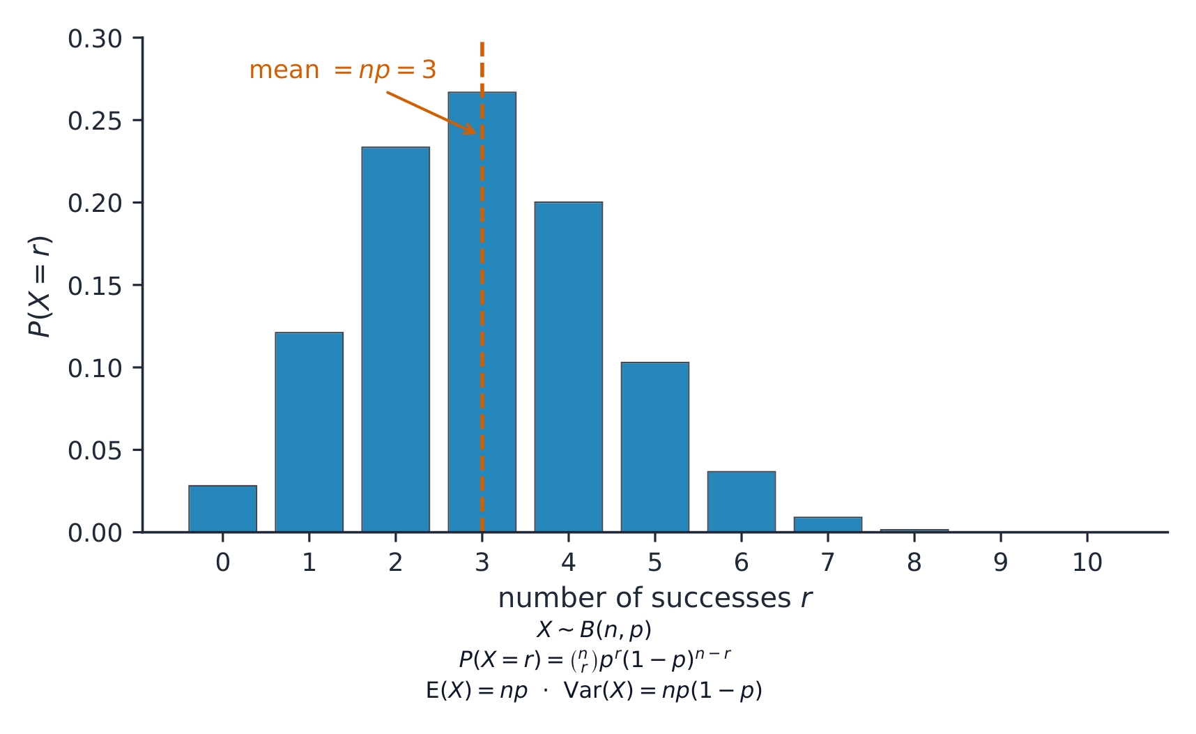
גרף עמודות של ההתפלגות הבינומית B(10, 0.3) עם הממוצע מסומן ב3
ההתפלגות $B(10,0.3)$: כל עמודה היא $P(X=r)$, מרוכזת סביב הממוצע $np=3$.
Explore · ⁨חקור⁩

A discrete distribution · ⁨התפלגות דיסקרטית⁩

Change n and p for a binomial distribution and watch the bars — the probability of each number of successes. · ⁨שנה את n ו-p עבור התפלגות בינומית וצפה בעמודות – ההסתברות של כל מספר הצלחות.⁩

Watch lesson · ⁨צפה בשיעור⁩
5.5

The normal distribution · ⁨ההתפלגות הנורמלית⁩

Syllabus · ⁨סיילבוס⁩
English
Candidates should be able to: Notes and examples
understand the use of a normal distribution to model a continuous random variable, and use normal distribution tables Sketches of normal curves to illustrate distributions or probabilities may be required.
solve problems concerning a variable $X$, where $X \sim N(\mu, \sigma^2)$, including: – finding the value of $P(X > x_1)$, or a related probability, given the values of $x_1$, $\mu$, $\sigma$. – finding a relationship between $x_1$, $\mu$ and $\sigma$ given the value of $P(X > x_1)$ or a related probability For calculations involving standardisation, full details of the working should be shown. e.g. $Z = \frac{(X - \mu)}{\sigma}$
recall conditions under which the normal distribution can be used as an approximation to the binomial distribution, and use this approximation, with a continuity correction, in solving problems. $n$ sufficiently large to ensure that both $np > 5$ and $nq > 5$.
עברית
המועמדים אמורים להיות מסוגלים: הערות לדוגמאות
הבנת השימוש בחלוקה נורמלית לדגם של משתנה אקראי רציף, והשתמש בטבלאות חלוקה נורמלית ייתכן שתידרש עריכת סקיצות של עקומות נורמליות כדי להמחיש חלוקות או סיכויים.
פתרון בעיות הקשורות למשתנה $X$, כאשר $X \sim N(\mu, \sigma^2)$, כולל: – מציאת הערך של $P(X > x_1)$, או סיכוי קשור, בהינתן הערכים של $x_1$, $\mu$, $\sigma$. – מציאת קשר בין $x_1$, $\mu$ ו$\sigma$ בהינתן הערך של $P(X > x_1)$ או סיכוי קשור לחישובים הקשורים בסטנדרטיזציה יש להציג פרטים מלאים של הפעולה. לדוגמה: $Z = \frac{(X - \mu)}{\sigma}$
זיכרון תנאים תחתיהם ניתן להשתמש בחלוקה הנורמלית כאפ approximate לחלוקה הדו-תוצאתית, והשתמש באפApproximation זו, עם תיקון רציפות, בפתרון בעיות. $n$ גדול מספיק כדי להבטיח שגם $np > 5$ וגם $nq > 5$.

Source: Cambridge International syllabus · ⁨מקור: הסיילבוס הבינלאומי של קמבריד'ג'⁩

English
The 68-95-99.7 rule

The normal distribution 正态分布 models a continuous random variable 连续型随机变量 with a symmetric bell shape. Write $X \sim N(\mu, \sigma^2)$, where $\mu$ is the mean and $\sigma$ is the standard deviation. To use the tables, by standardisation 标准化 convert to the variable $Z \sim N(0, 1)$:

$$Z = \frac{X - \mu}{\sigma}.$$

Then $P(X < x) = P\!\left(Z < \dfrac{x - \mu}{\sigma}\right)$, which you read from the normal table $\Phi$.

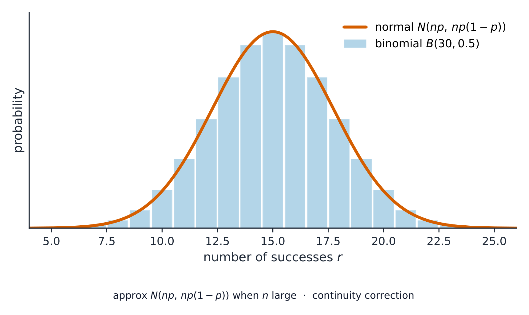
The normal distribution is also a good approximation 近似 to the binomial when $n$ is large. Because you replace a discrete variable by a continuous one, apply a continuity correction 连续性校正 (adjust by $0.5$).

Worked example. Bags of rice have mass $X \sim N(\mu, 0.14^2)$. Given that $P(X < 1.48) = 0.22$, find $\mu$.

From the table, $P(Z < z) = 0.22$ gives $z = -0.772$. So

$$\frac{1.48 - \mu}{0.14} = -0.772 \;\Rightarrow\; \mu = 1.48 + 0.772 \times 0.14 = 1.59\ \text{kg (3 s.f.)}.$$

עברית
חוק ה-68-95-99.7
לוח גלטון עם כדורים היוצרים צורת פעמון
לוח גלטון: כדורים הצופלים דרך סיכות מצטברים להתפלגות נורמלית בצורת פעמון.

ההתפלגות הנורמלית מדגמת משתנה מקרי רציף בעל צורת פעמון סימטרית. כתוב $X \sim N(\mu, \sigma^2)$, כאשר $\mu$ הוא הממוצע ו$\sigma$ הוא הסטיית התקן. כדי להשתמש בטבלאות, באמצעות סטנדרטיזציה המר את המשתנה ל$Z \sim N(0, 1)$:

$$Z = \frac{X - \mu}{\sigma}.$$

אז $P(X < x) = P\!\left(Z < \dfrac{x - \mu}{\sigma}\right)$, שנקרא מהטבלה הנורמלית $\Phi$.

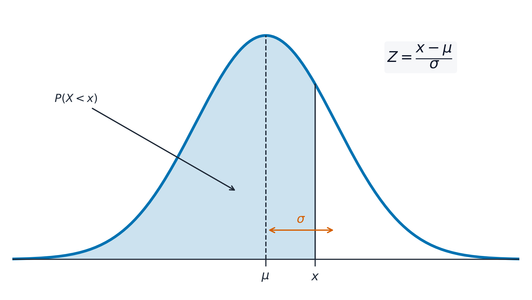
עקומת פעמון סימטרית שמרכזה הממוצע עם השטח עד לערך x מוצל
הסתברות נורמלית היא שטח מתחת לעקומת הפעמון; סטנדרטיזציה משנה את קנה המידה שלה ל$Z\sim N(0,1)$.

ההתפלגות הנורמלית היא גם קירוב טוב להתפלגות דו-ספוגית כאשר $n$ גדול. מכיוון שאתה מחליף משתנה דיסקרטי ברציף, יש להפעיל תיקון רציפות (שינוי ב$0.5$).

עמודות של התפלגות דו-ספוגית עם עקומה נורמלית תואמת מצוירות מעליהן
כאשר $n$ גדול, עמודות ההתפלגות הדו-ספוגית עוקבות אחרי עקומה נורמלית באותו ממוצע ושונות.

דוגמה פתורה. שקיות אורז יש להן מסה $X \sim N(\mu, 0.14^2)$. נתון כי $P(X < 1.48) = 0.22$, מצא $\mu$.

מהטבלה, $P(Z < z) = 0.22$ נותן $z = -0.772$. לכן

$$\frac{1.48 - \mu}{0.14} = -0.772 \;\Rightarrow\; \mu = 1.48 + 0.772 \times 0.14 = 1.59\ \text{kg (3 s.f.)}.$$

Explore · ⁨חקור⁩

The normal distribution · ⁨החלוקה הנורמלית⁩

Shade the area to find a probability. A z-value measures how many standard deviations a point is from the mean. · ⁨צל את השטח כדי למצוא הסתברות. ערך z מדד כמה סטיות תקן נקודה נמצאת מהמוצע.⁩

Vocabulary · ⁨מילון מונחים⁩ Train · ⁨אימון⁩
English עברית
normal distribution/ˈnɔːml ˌdɪstrɪˈbjuːʃn/ התפלגות נורמלית
continuous random variable/kənˈtɪnjuːəs ˈrændəm ˈveərɪəbl/ משתנה אקראי רציף
standardisation/ˌstændədaɪˈzeɪʃn/ סטנדרטיזציה
approximation/əˌprɒksɪˈmeɪʃn/ הנחה
continuity correction/kɒntɪˈnjuːɪti kəˈrekʃn/ תיקון רציפות
Probability & Statistics/ˌprɒbəˈbɪlɪti ænd stəˈtɪstɪks/ הסתברות וסטטיסטיקה
central tendency/ˈsentrəl ˈtendənsi/ מיקום מרכזי
Watch lesson · ⁨צפה בשיעור⁩
5.5

Exam tips · ⁨טיפים לבחינות⁩

English
  • Decide whether order matters: permutations ($^nP_r$) when it does, combinations ($^nC_r$) when it does not.
  • For a discrete random variable, check the probabilities sum to $1$ and use $E(X) = \sum x\,P(X=x)$.
  • For the normal distribution, standardise with $z = (x - \mu)/\sigma$, sketch and shade, then read the table.
  • Apply a continuity correction when approximating a discrete variable by the normal.
עברית
  • החלט האם סדר חשוב: פרמוטציות ($^nP_r$) כשכן, קומבינציות ($^nC_r$) כשהלא.
  • עבור משתנה מקרי דיסקרטי, בדוק שהסתברויות סוכמות ל$1$ והשתמש ב$E(X) = \sum x\,P(X=x)$.
  • עבור ההתפלגות הנורמלית, סטנדרטיזציה עם $z = (x - \mu)/\sigma$, שרטוט והצללה, ואז קריאת הטבלה.
  • הפעל תיקון רציפות בקירוב משתנה דיסקרטי על ידי הנורמלית.

Interactive lessons on this topic · ⁨שיעורים אינטראקטיביים בנושא זה⁩

Work through it step by step, with instant-check exercises. · ⁨לעבור על הדברים צעד אחר צעד, עם תרגילים לבדיקה מיידית.⁩

Past Papers · ⁨מבחני עבר⁩

More topics in A-Level Mathematics · ⁨מתמטיקה A-Level⁩ · ⁨נושאים נוספים בA-Level Mathematics · ⁨מתמטיקה A-Level⁩⁩

Log in or create account · ⁨היכנס או צור חשבון⁩

IGCSE, A-Level & AP