From an ice pack to a star
An ice pack, a swinging bridge and a distant star all involve energy. This unit links molecular motion, nuclear changes, oscillations and astronomical observations. The task is often to test a claim, not just calculate a number: state the model, carry units through the calculation, then compare your result with the claim.
WPH15 covers statements 125–171 of Pearson Issue 3. It also uses Units 1, 2 and 4. Work through sheets 5.1–5.9 before their matching authentic sets. Use the supplied constants consistently: $g=9.81\ \mathrm{m\,s^{-2}}$, $k_B=1.38\times10^{-23}\ \mathrm{J\,K^{-1}}$ and $G=6.67\times10^{-11}\ \mathrm{N\,m^2\,kg^{-2}}$ unless the question gives a different local value. Here $k_B$ is the Boltzmann constant; $k_s$ denotes a spring constant.
Heating, phase change and thermistor calibration
Follow the energy, not only the temperature
Internal energy 内能 is the total energy in the random motion and interactions of molecules: random kinetic energy plus intermolecular potential energy. It excludes the kinetic energy of the whole object moving together. Temperature relates to average random molecular kinetic energy, not total internal energy. Two samples at the same temperature can have different internal energies because their amounts and states differ.
Specific heat capacity 比热容 $c$ is the energy needed per kilogram for a one-kelvin temperature rise without a change of state. Specific latent heat 比潜热 $L$ is the energy transferred per kilogram during a particular change of state at constant temperature.
A temperature difference of $1\ ^\circ\mathrm C$ equals a difference of $1\ \mathrm K$. Absolute temperatures in gas and radiation laws must be kelvin. During melting or boiling, energy changes molecular arrangements and potential energy while temperature remains constant in the ideal constant-pressure phase change. An ice pack absorbs energy from the food/surroundings as it melts. It does not send “cold energy” into the food.
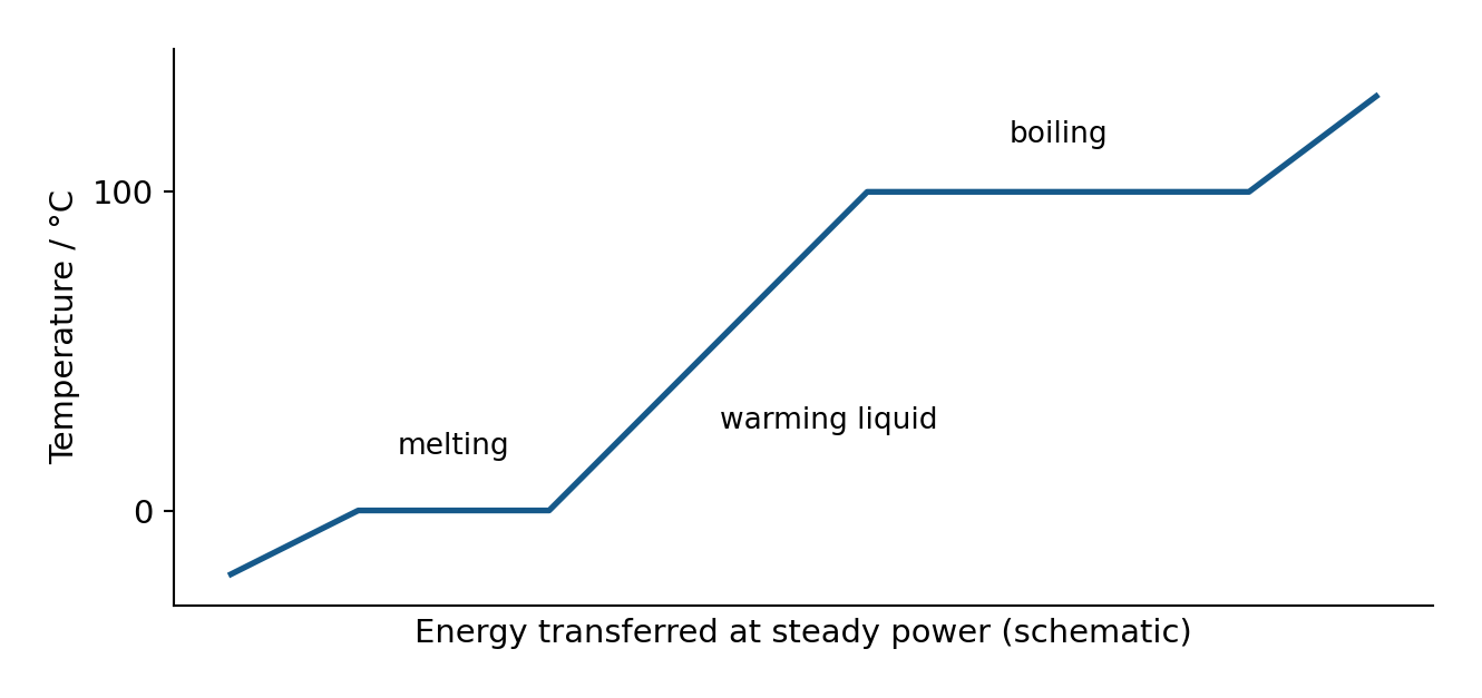
At constant heating power, steeper temperature–time gradients mean smaller $mc$, provided heat loss is negligible. A flat section does not mean that energy transfer has stopped. For a heater, input energy is $E_{\rm in}=Pt=VIt$; useful thermal energy can be smaller because energy escapes to surroundings.
Worked example. A $0.40\ \mathrm{kg}$ block of ice at $-10\ ^\circ\mathrm C$ melts to water at $0\ ^\circ\mathrm C$. Use $c_{\rm ice}=2100\ \mathrm{J\,kg^{-1}\,K^{-1}}$ and $L_f=3.4\times10^5\ \mathrm{J\,kg^{-1}}$.
Known: mass, initial/final temperatures and material constants. Why: warming the solid and melting it are separate energy transfers.
Worked example. A $1000\ \mathrm W$ heater boils away $0.20\ \mathrm{kg}$ of water in $600\ \mathrm s$. Find efficiency, using $L_v=2.26\times10^6\ \mathrm{J\,kg^{-1}}$.
For repeated kettle loads, calculate total water volume, number of loads and total operating time. Compare energies over the same stated interval. Standby loss over a day and input needed to boil water are different quantities; state what a particular comparison actually establishes.
CP12: calibrate a thermostat
A thermistor 热敏电阻 has resistance that changes with temperature. The usual negative-temperature-coefficient (NTC) thermistor decreases in resistance when heated. In a potential divider 分压器:
With the thermistor as the lower resistor and output measured across it, warming reduces output voltage. Swapping resistor positions reverses that trend. A thermostat switches at a chosen output threshold; the divider alone is not a complete switching device.
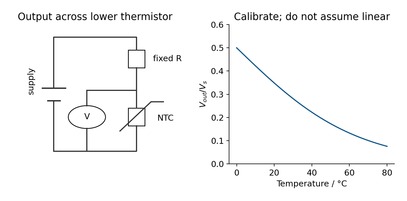
For core practical 12, place the thermistor and a reference thermometer close together in a stirred water bath. Keep electrical contacts dry and insulated. At several temperatures across the intended range, wait for thermal equilibrium and record temperature and divider voltage. Keep supply voltage and fixed resistance unchanged. Use a high-input-resistance voltmeter to reduce loading. Plot output against temperature and interpolate the voltage for the chosen switching temperature. Repeat readings or compare warming/cooling to reveal lag. Do not assume a linear calibration without evidence. Use low-voltage electricity and take care with hot water.
CP13: measure latent heat
Supply measured electrical power to a material during its phase change. Measure mass melted or evaporated over a timed interval after conditions stabilise. A balance measures mass change; do not confuse collected liquid volume with mass. Without loss correction, $L=VIt/\Delta m$ assumes all supplied energy causes the phase change.
A useful correction is to compare two powers at the same steady phase-change temperature. If heat-loss power is approximately unchanged, subtracting the two measurements removes it:
State that constant-loss assumption. A control measurement of melting without the heater is another possible correction in a suitable ice experiment. Reduce heat loss with insulation where safe; avoid splashing, hot surfaces and unsafe mains connections.
Ideal gases and molecular kinetic energy
Kelvin and the ideal-gas model
Absolute zero 绝对零度 is $0\ \mathrm K$, about $-273\ ^\circ\mathrm C$. It is the lower limit of thermodynamic temperature. In the classical ideal-gas model, average translational kinetic energy tends to zero as temperature tends to zero. Real gases condense before that extrapolation is reached; do not claim molecules in every real material lose all possible energy.
Absolute temperature 绝对温度 is measured in kelvin: $T=\theta_{^\circ\mathrm C}+273$ to the precision normally used here. An ideal gas 理想气体 consists of particles with negligible volume, no intermolecular forces except during elastic collisions, and random motion. Pressure comes from momentum changes at walls.
Here $N$ is the number of molecules, not the number of moles. Use pressure in pascals, volume in cubic metres and temperature in kelvin. For a fixed number of molecules:
At fixed volume, pressure is proportional to kelvin temperature. At fixed temperature, $pV$ is constant. Include external pressure if a gauge reports pressure relative to the atmosphere.
Worked example. A rigid $2.0\times10^{-3}\ \mathrm{m^3}$ vessel contains gas at $1.0\times10^5\ \mathrm{Pa}$ and $300\ \mathrm K$. Find $N$ and pressure after warming to $360\ \mathrm K$.
If one molecule has mass $m_0$, total gas mass is $Nm_0$. For a sphere, first find $V=4\pi r^3/3$; radius is half the diameter.
Derive the molecular energy relation
The kinetic-theory pressure relation is $pV=\tfrac13Nm_0\langle c^2\rangle$, where $\langle c^2\rangle$ is mean square speed 速率平方的平均值. It follows from elastic momentum changes at a wall and equal mean squared motion in the three perpendicular directions. The root mean square speed 方均根速率 is $c_{\rm rms}=\sqrt{\langle c^2\rangle}$; it is not the square of mean speed.
For a cube of side $l$, one molecule with velocity component $c_x$ changes wall momentum by $2m_0c_x$ at each elastic collision. Its return time to that same wall is $2l/c_x$. Hence its average force is $m_0c_x^2/l$. Sum over molecules and divide by wall area $l^2$:
Random motion is equally distributed among perpendicular directions, so $\langle c^2\rangle=3\langle c_x^2\rangle$. This gives the pressure relation above. Equate the two expressions for $pV$, cancel $N$, then rearrange:
At one temperature, different gas species have equal mean translational kinetic energies, but lighter molecules have greater RMS speeds. If speed doubles at the same temperature, molecular mass is one quarter. Heating increases average molecular kinetic energy; it does not give every molecule the same speed.
CP14: pressure and volume at fixed temperature
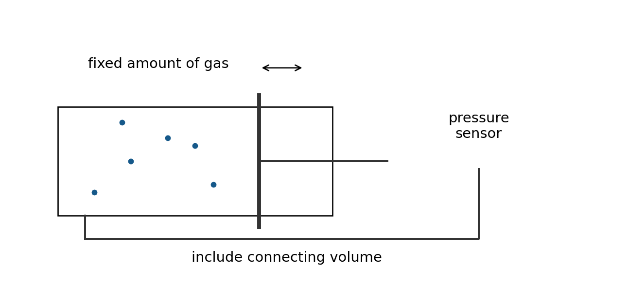
Trap a fixed amount of gas in a syringe or calibrated cylinder connected to a pressure sensor. Check calibration and use absolute pressure. Include connecting-tube dead volume where significant. Change volume gradually, wait after each change for temperature to return to the surroundings, then record several pressure–volume pairs. Do not let gas escape. A plot of $p$ against $1/V$ should be straight through the origin within uncertainty. A $p$–$V$ curve is not straight. Avoid excessive pressure and secure connections. Rapid compression heats the gas and breaks the intended constant-temperature condition.
Binding energy, fission and fusion
Mass deficit is an energy difference
A nucleus contains $Z$ protons and $A-Z$ neutrons. Its mass is smaller than the total mass of these free nucleons. This mass deficit 质量亏损 corresponds to the binding energy 结合能 needed to separate the nucleus completely into free nucleons:
Here $c_0$ is the speed of light, distinguished from specific heat capacity. The unified atomic mass unit 统一原子质量单位 is $1\ \mathrm u=1.66\times10^{-27}\ \mathrm{kg}$. Convert all masses to the same unit before subtracting. Nuclear masses and neutral-atom masses are not interchangeable without accounting consistently for electrons. Use the masses the question actually supplies.
Worked example. A nucleus has mass deficit $0.030\ \mathrm u$ and $A=4$. Find binding energy per nucleon.
Why fusion and fission can both release energy
The binding-energy-per-nucleon curve rises steeply for light nuclei, peaks near iron/nickel, then decreases gradually for heavy nuclei. Greater binding energy per nucleon generally means nucleons are more tightly bound. It is the vertical value, not just mass number, that matters when comparing points.
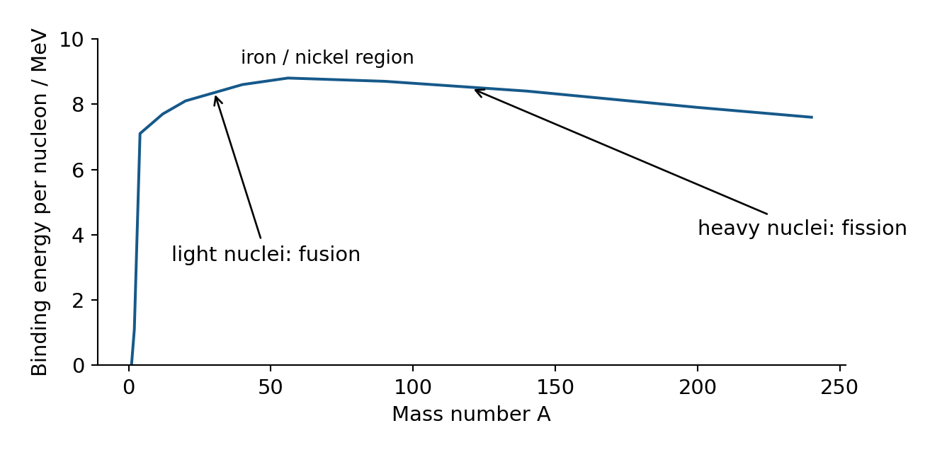
Nuclear fusion 核聚变 combines light nuclei. Nuclear fission 核裂变 splits a heavy nucleus into smaller products, often with neutrons. Energy is released when the products have greater total binding energy and smaller total rest mass than the reactants. For a reaction, calculate the total mass difference, not merely a difference of two per-nucleon values. Total energy is conserved.
Fusion needs very high temperature to give nuclei enough kinetic energy to approach despite electrostatic repulsion, and high density/confinement to make enough close encounters and sustain energy release. Temperature and density have different roles. Merely naming “high pressure” does not explain overcoming repulsion.
Radiation, background and decay
Choose radiation by its interaction
Alpha radiation 阿尔法辐射 consists of helium nuclei: strongly ionising, short range and stopped by paper or a few centimetres of air. Beta radiation 贝塔辐射 consists of electrons or positrons: less ionising, more penetrating, typically stopped by a few millimetres of aluminium. Gamma radiation 伽马辐射 is electromagnetic radiation: weakly ionising and highly penetrating; lead or concrete reduces its intensity but does not provide a sharp stopping thickness.
In a cloud chamber, alpha tracks are thick mainly because of strong ionisation, and relatively straight because the particles have large mass compared with beta particles. Beta tracks are thinner and more easily deflected. Do not swap these explanations. Beta radiation can monitor paper thickness because some passes through and some is absorbed; a change in thickness changes the transmitted count rate.
In nuclear equations 核反应方程, conserve nucleon number and charge number. Beta-minus decay converts a neutron to a proton; the mass number stays the same and atomic number increases by one. Include the antineutrino where required, as in Unit 4:
Alpha decay reduces $A$ by four and $Z$ by two. Gamma emission changes neither $A$ nor $Z$. Nuclear equations conserve more than these two numbers: energy and momentum still matter.
Correct background before applying a model
Background radiation 本底辐射 comes from sources such as rocks, cosmic rays and the environment. Measure it for a sufficiently long time with the test source absent. Subtract its count rate from every source-plus-background reading. Keep counting-time units consistent. Corrected detector count rate is proportional to source activity only when geometry and detection efficiency remain unchanged; it is not automatically the activity in becquerels.
Worked example. A detector reads $62\ \mathrm{min^{-1}}$ at distance $r$, including background $14\ \mathrm{min^{-1}}$. Predict total rate at $2r$ for a small isotropic gamma source with negligible absorption.
Do not divide the background by four: it is not all coming from the test source.
Random events, predictable populations
Radioactive decay 放射性衰变 is spontaneous: an unstable nucleus decays without an external trigger. It is random: the exact time for an individual nucleus cannot be predicted. A large population has a predictable statistical decay pattern. Activity 放射性活度 $A$ is the number of decays per second, measured in becquerels 贝可勒尔, $1\ \mathrm{Bq}=1\ \mathrm{s^{-1}}$.
The decay constant 衰变常数 $\lambda$ is the probability per unit time of decay for a nucleus. The half-life 半衰期 $t_{1/2}$ is the time for the undecayed population, or activity, to halve on average.
At one half-life, $N/N_0=1/2=e^{-\lambda t_{1/2}}$. Taking logs gives:
A log-activity–time line has gradient $-\lambda$. Take logarithms of corrected rates, not source-plus-background readings. Read several half-life intervals from a graph and average; measure from the corrected activity level, not from zero total counts.
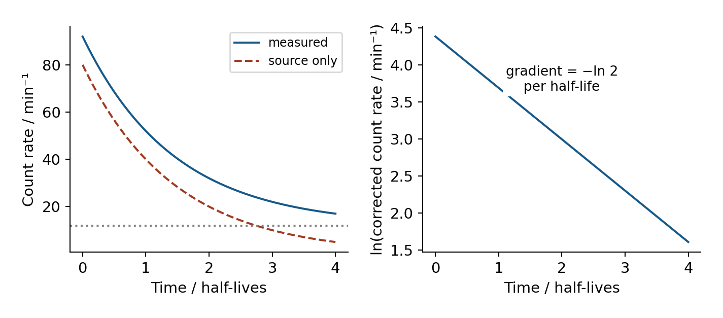
Worked example. A source has half-life $3.0\ \mathrm{years}$. When will activity fall to $2.0\%$ of its initial value?
Use a fraction, not $2.0$ inside the logarithm. If calculating power from a radioactive source, $P=A E_{\rm decay}$, with energy per decay in joules. This is released nuclear power; useful electrical output may be smaller. Convert the half-life to seconds when activity must be in becquerels.
CP15: absorption of gamma radiation by lead
Keep source, absorber and detector in fixed positions. Measure background, then counts over equal known intervals for several total lead thicknesses. Repeat or extend the counting time because counts fluctuate. Subtract background rate before comparing transmission. If each equal thickness gives the same fractional reduction, the attenuation is exponential; a graph of log corrected rate against thickness is approximately straight. Three half-value thicknesses transmit $1/8$, not $1/3$.
The material-absorption constant is not the time-decay constant of the source. Avoid readings too close to background, where subtraction gives large relative uncertainty. Handle sources with the specified tools under supervision, keep distance, minimise exposure time and return them to shielding. Never touch a source or direct it at people. Keep lead handling clean and wash hands.
Simple harmonic motion, graphs and energy
The restoring condition
Simple harmonic motion 简谐运动 (SHM) occurs when resultant acceleration is proportional to displacement from a fixed equilibrium position and directed towards it:
The negative sign is the restoring direction. Constant speed, repetition alone or a force merely pointing towards a centre does not establish SHM. For a vertically hanging spring, measure $x$ from the loaded equilibrium position. Weight is already balanced there; the resultant for displacement is $-k_sx$.
For release from positive maximum displacement at $t=0$:
Here $A_0$ is amplitude, not radioactive activity. The phase depends on the chosen starting time; a sine displacement can describe the same motion with another origin. Differentiate graphically: the displacement–time gradient is velocity, and velocity–time gradient is acceleration. At maximum displacement, speed is zero and acceleration points back towards equilibrium. At equilibrium, speed is greatest and acceleration is zero.
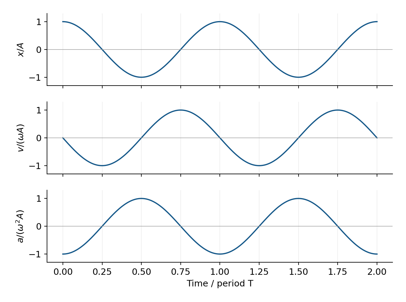
Worked example. A graph gives amplitude $0.030\ \mathrm m$ and period $0.50\ \mathrm s$. Find maximum speed and acceleration.
Alternatively find maximum speed from a tangent to the displacement graph at equilibrium. Convert centimetres to metres. A negative straight $a$–$x$ gradient is $-\omega^2$, so take its negative before the square root.
Periods and energy
For a mass on an ideal spring and for a simple pendulum at small angles:
Pendulum length is pivot to bob centre. The small-angle period does not depend on bob mass. A period ratio for one unchanged spring gives $T_2/T_1=\sqrt{m_2/m_1}$. Use total new mass before finding added mass.
Worked example. A $0.50\ \mathrm{kg}$ mass has period $0.80\ \mathrm s$. An extra mass increases the period to $1.00\ \mathrm s$ on the same spring.
For an undamped spring oscillator, energy transfers between elastic potential and kinetic stores:
Thus the $E_k$–$x$ graph is an inverted parabola: zero at $\pm A_0$, positive maximum at $x=0$. The $E_p$–$x$ graph opens upwards. Their sum is constant in the undamped model. In a damped system energy is transferred out, so amplitude decreases. Total energy including surroundings remains conserved.
CP16: infer an unknown mass from resonance
Keep the same spring/support system. Attach several known masses, drive with small oscillations and vary frequency to find the largest steady amplitude for each mass. Record the resonant frequency, repeating slowly around each peak. With light damping it approximates natural frequency. Plot $1/f^2$ against total known mass; the spring model gives gradient $4\pi^2/k_s$. Use the calibration to infer an unknown mass from its resonant frequency.
Account for a hanger and, where significant, the effective moving mass of the spring. A nonzero intercept may represent this contribution; do not force the line through the origin without justification. Keep amplitudes small and below the elastic limit. Secure masses and stand, and keep feet clear. Measuring free periods can provide a useful independent comparison, but the specified practical uses resonant frequencies.
Forced oscillations, resonance and damping
A free oscillation 自由振动 follows an initial disturbance without continued periodic driving. A forced oscillation 受迫振动 is maintained by a periodic driving force; its steady frequency is the driving frequency. Natural frequency 固有频率 is the frequency of free oscillation for the system under the stated conditions.
Resonance 共振 occurs when driving frequency is at or near natural frequency, giving efficient energy transfer and a large steady amplitude. It does not mean “maximum frequency”. For a lightly damped system, the amplitude peak is near the undamped natural frequency. Greater damping lowers and broadens the peak; do not present every damped peak as exactly at the undamped natural frequency.
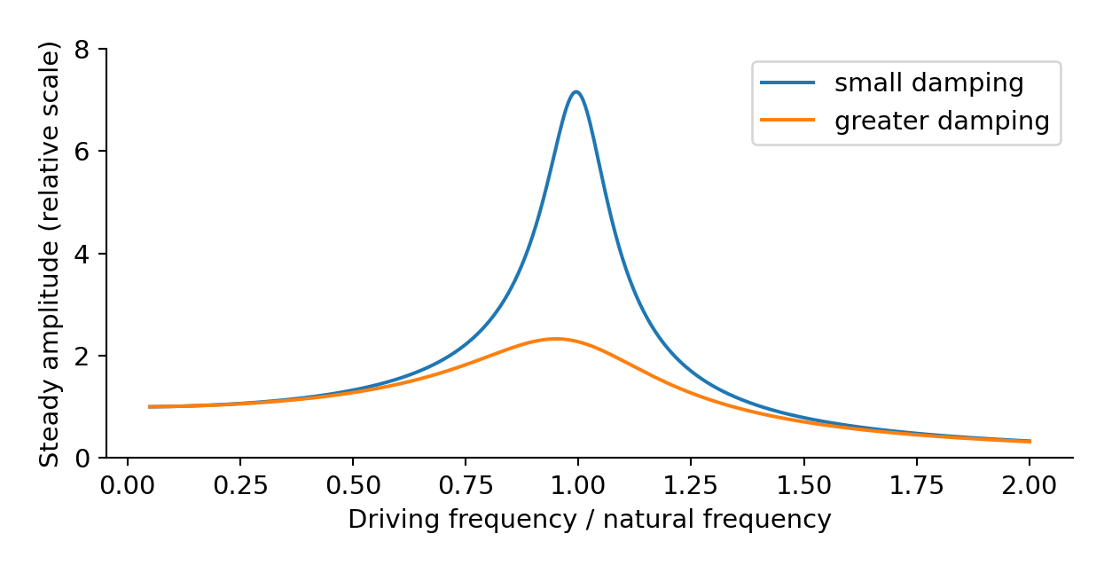
Damping 阻尼 transfers energy away from oscillation, for example through resistive work that increases the thermal energy of dampers and surroundings. Stronger damping can reduce dangerous bridge/building motion. Plastic deformation 塑性形变 of a ductile material also absorbs mechanical energy irreversibly; purely elastic deformation returns stored energy and is not the same mechanism.
Worked explanation. People walking supply a periodic driving force to a bridge. If its frequency is near a natural frequency, energy transfers efficiently into the bridge and amplitude increases. Dampers do work against motion, transferring oscillation energy to thermal stores, so the steady amplitude is limited. Link cause and effect in this order rather than listing “resonance, energy, damping”.
For the same shape and amplitude, adding mass to a light pendulum increases its stored mechanical energy while the small-angle ideal period remains unchanged. Under comparable resistive losses it can lose a smaller fraction of energy per cycle. That contextual damping comparison does not prove that every heavier oscillator always damps more slowly.
Gravitational fields and orbits
Field and potential have different meanings
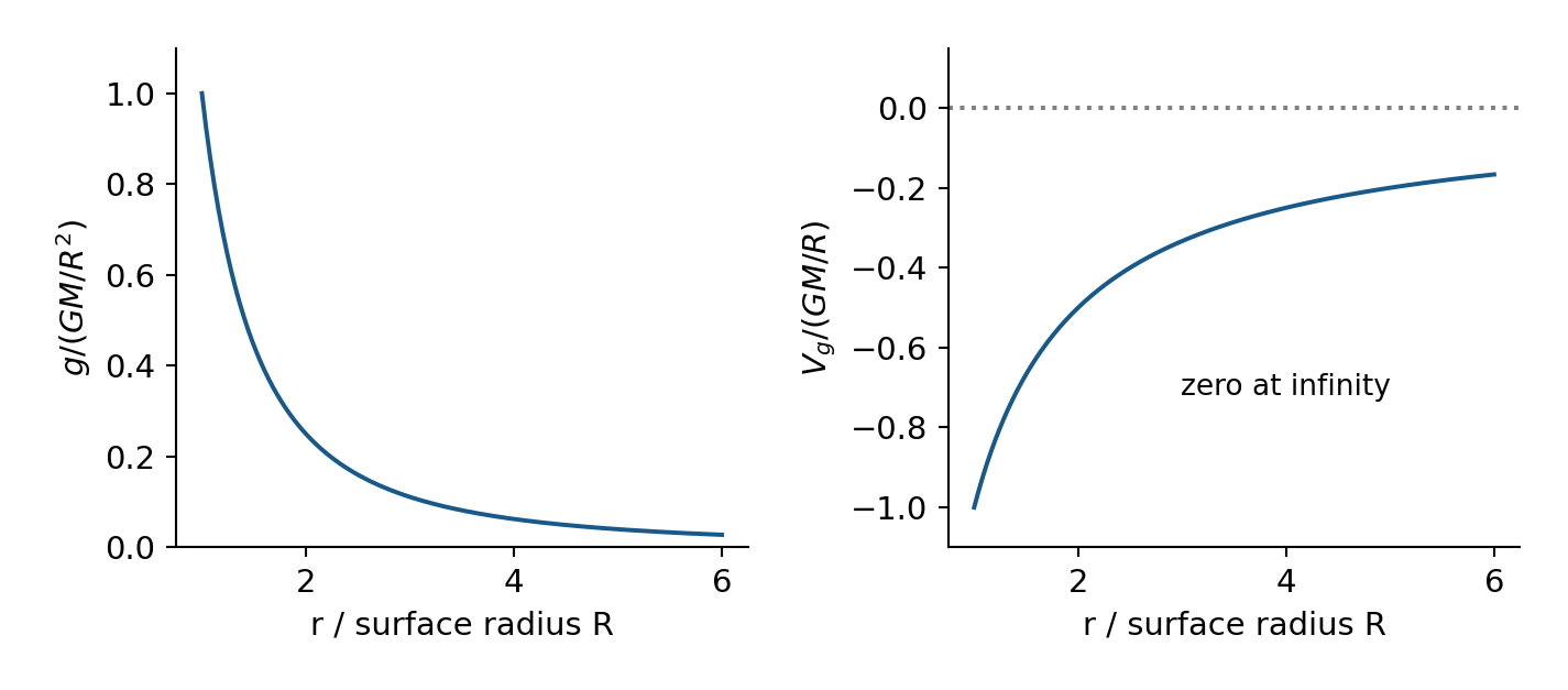
A gravitational field 引力场 is a region where a mass experiences a force. Gravitational field strength 重力场强度 $g=F/m$ is force per unit test mass. It is a vector pointing towards an isolated source mass. Newton's law for point masses, or outside a spherical symmetric source, is:
$r$ is centre-to-centre distance, not height above the surface. For near-Earth local motion, constant $g$ can be suitable. Over large radial distances it is not constant.
Gravitational potential 引力势 is potential energy per unit mass, with zero at infinity:
Potential is a scalar and negative at finite distance. Moving outward makes it less negative, so potential energy increases while attractive force weakens. A potential graph value and its corresponding radius give $M=-Vr/G$.
Gravity and electric fields are both radial for isolated point sources and their force magnitudes obey inverse-square laws. Gravity acts on mass and is attractive in this model. Electric force acts on charge and can attract or repel. Electric field direction follows the force on positive test charge; a negative charge is forced oppositely.
Worked example. A $1000\ \mathrm{kg}$ satellite moves from radius $r_1=6.4\times10^6\ \mathrm m$ to $r_2=1.28\times10^7\ \mathrm m$ around Earth, $M=6.0\times10^{24}\ \mathrm{kg}$. Find its potential-energy change.
The positive sign is final minus initial. This is not the total launch energy, since kinetic energy may also change. $mg\Delta h$ with constant surface $g$ is unsuitable over this distance.
Derive a circular orbit
The gravitational force supplies the inward resultant:
Orbiting mass cancels. The period grows with radius. To appear stationary above one point on a rotating planet, a satellite needs a circular equatorial orbit, the same rotational direction and matching angular velocity/period. Matching period alone is insufficient.
Worked example. For $GM=4.00\times10^{14}\ \mathrm{m^3\,s^{-2}}$ and period $T=8.64\times10^4\ \mathrm s$, find stationary-orbit radius.
Subtract planet radius only if asked for height above the surface. For a star's surface field, use its radius, not its listed diameter; test a multiple-of-Earth-field claim by calculating the ratio.
Stellar radiation, distances and evolution
Temperature, luminosity and received intensity
A black body 黑体 absorbs all incident electromagnetic radiation and is an ideal thermal emitter. Its continuous spectrum has a characteristic shape. Increasing temperature increases total emitted power per unit area and moves the wavelength peak to shorter wavelength. The area under a spectral-intensity curve represents total intensity only with the appropriate spectral-axis definition.
Luminosity 光度 $L_\star$ is total power emitted. Intensity 强度 $I$ received at distance $d$ is power per unit receiving area. For a spherical black-body star of radius $R$ radiating equally in all directions:
The first area is the emitting surface; the second is the expanding receiving sphere. Do not substitute observer distance into the star's surface area. Real emitters may not be perfect black bodies, and intervening material can absorb radiation.
Wien's stated constant describes a spectrum per unit wavelength. A maximum of a spectrum plotted per unit frequency does not transform into that wavelength maximum simply by replacing $\lambda$ with $c_0/f$. If an exam gives the frequency corresponding to its specified wavelength peak, convert that given wavelength using $c_0=f\lambda$. Do not turn that particular task convention into a general rule for every spectral plot.
Worked example. A star's wavelength spectrum peaks at $580\ \mathrm{nm}$ and its radius is $7.0\times10^8\ \mathrm m$. Find temperature, luminosity and intensity at $1.5\times10^{11}\ \mathrm m$.
Keep unrounded temperature because it is raised to the fourth power. Compare the received intensity with the stated reference before accepting a planetary-temperature or power claim.
Two distance methods
Trigonometric parallax 三角视差 measures a nearby star's apparent angular shift against distant background stars as Earth moves around the Sun. Observations six months apart use a baseline of two Earth-orbit radii. The parallax angle $p$ is half the total shift. For small $p$ in radians, distance is $d\approx r_{\rm orbit}/p$. A parsec 秒差距 is the distance giving parallax $1$ arcsecond; $d_{\rm pc}=1/p_{\rm arcsec}$. Do not use the diameter of Earth or Sun as the orbital baseline.
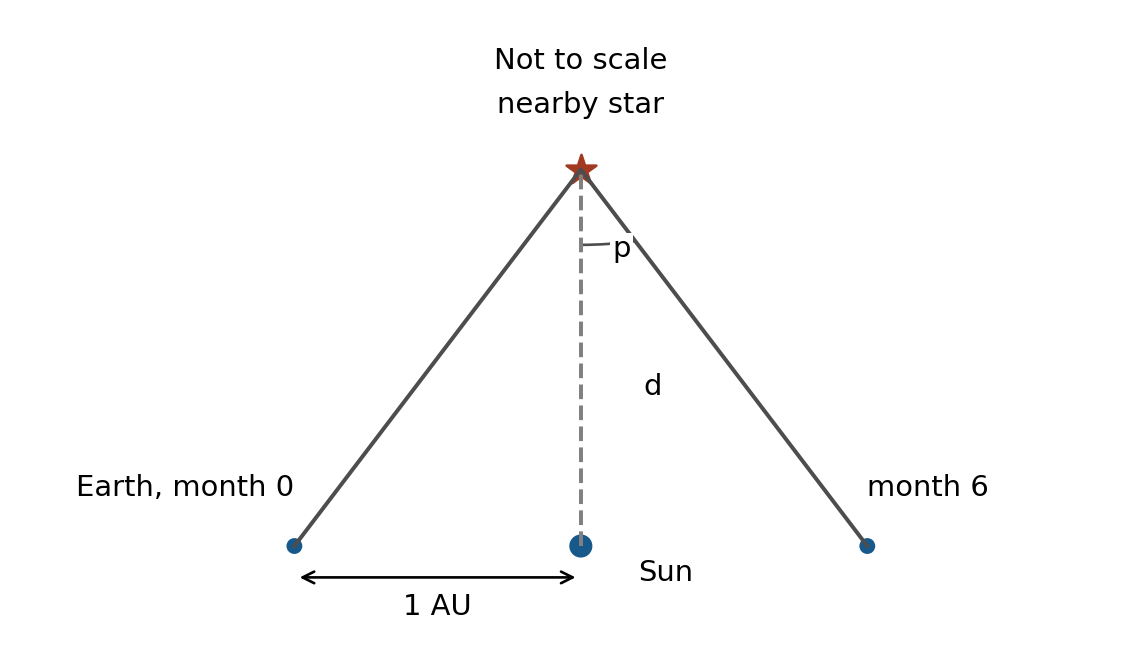
At large distance, $p$ becomes too small for the instrument to measure accurately. The limitation is angular resolution/relative uncertainty, not necessarily that the star is invisible.
A standard candle 标准烛光 is an object of known luminosity. Identify one in a cluster, measure received intensity and use $d=\sqrt{L_\star/(4\pi I)}$. Its apparent brightness is not assumed known beforehand. Cepheid variable stars have a calibrated relationship between period and luminosity. Measure several complete light-curve periods, divide by their number, read the calibration carefully and convert any solar-luminosity units. A straight line on log axes is not automatically a linear relationship between the raw quantities.
Worked example. A standard candle has $L_\star=4.0\times10^{28}\ \mathrm W$ and received intensity $2.0\times10^{-10}\ \mathrm{W\,m^{-2}}$.
Read the Hertzsprung–Russell diagram
A Hertzsprung–Russell diagram 赫罗图 plots luminosity vertically against surface temperature horizontally, usually with temperature decreasing to the right and logarithmic scales. The main sequence 主序星带 runs from hot, bright stars at upper left to cool, faint stars at lower right. Red giants 红巨星 are cool but luminous because of their large surface areas. White dwarfs 白矮星 are hot but faint because of their small surface areas. Mark the Sun near one solar luminosity and about $5800\ \mathrm K$ on the main sequence.
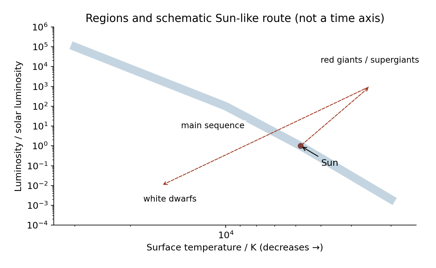
Stars form when gravity contracts a cloud of gas and dust. The core heats until hydrogen fusion can sustain a main-sequence star; outward pressure balances gravity. In a Sun-like star, core hydrogen eventually runs low, fusion there decreases and gravity contracts the core. Core temperature rises; shell hydrogen burning and later helium fusion are associated with expansion to a red giant. Outer layers are lost, leaving a white-dwarf core with no sustained fusion. It cools over a very long time. The Sun does not become a supernova or a neutron star.
A much more massive star can fuse heavier elements through later stages. When its core can no longer gain energy from fusion, collapse and a supernova can leave a neutron star or black hole, depending on the remnant. A massive main-sequence star has more fuel but consumes it much faster because of its hotter core. Its main-sequence lifetime can therefore be shorter. Explain fusion rate, not just fuel amount. An HR track shows changing temperature/luminosity, not a star travelling across space.
Doppler shifts and cosmology
Compare the same spectral line
The Doppler effect 多普勒效应 is a change in observed frequency/wavelength caused by relative motion along the line of sight. Successive wavefronts arrive farther apart from a receding source and closer together from an approaching source. Recession gives longer wavelengths and lower frequencies; approach gives shorter wavelengths and higher frequencies. Motion purely perpendicular to the line of sight is not the recession speed in the simple model.
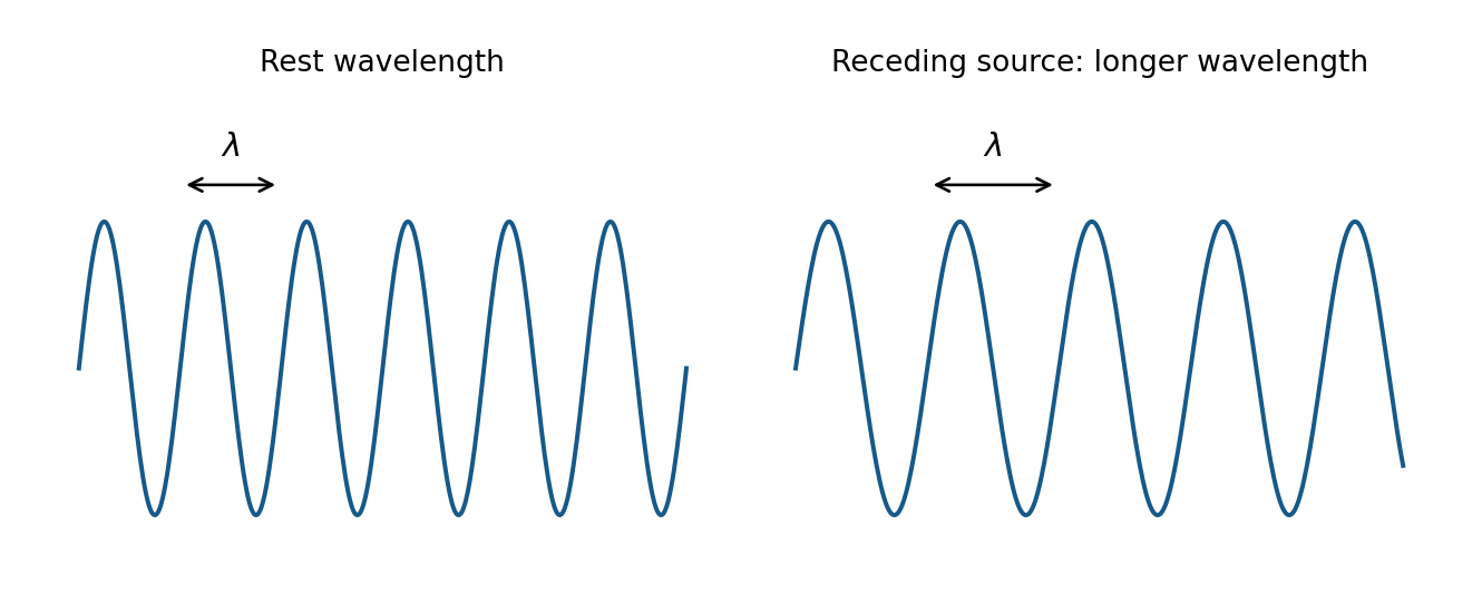
For electromagnetic radiation at low recession speeds:
Redshift 红移 $z$ is positive for recession. For small shifts, its magnitude also approximately equals the fractional decrease of observed frequency relative to emitted frequency. State the sign convention: $(f_{\rm observed}-f_{\rm rest})/f_{\rm rest}$ is negative for recession. Do not equate a positive redshift to a signed frequency increase. The approximation $v/c_0$ is not a general high-speed relativistic formula.
Worked example. A line emitted at $500\ \mathrm{nm}$ is observed at $505\ \mathrm{nm}$.
To use a star's absorption lines, recall Unit 2: photons are absorbed only when their energies match allowed atomic-level differences. Compare the same identified spectral line, not two different elements.
For opposite limbs of a rotating star, one approaches while the other recedes. If their shifts are equal and opposite, the separation of the two observed wavelengths is twice the shift of either limb. Halve that separation before finding the equatorial speed. Then use $T=2\pi R/v$. This assumes the observed line-of-sight limb speed represents the equatorial rotation speed under the stated viewing geometry.
Hubble law and its limits
On large cosmological scales, recession speed approximately follows Hubble's law 哈勃定律:
The Hubble constant 哈勃常数 $H_0$ has units of inverse time. In $\mathrm{km\,s^{-1}\,Mpc^{-1}}$, convert kilometres to metres and megaparsecs to metres before taking its reciprocal in seconds. Nearby objects may have local motions that do not follow the large-scale relationship.
Worked example. Use $H_0=70\ \mathrm{km\,s^{-1}\,Mpc^{-1}}$ and $1\ \mathrm{Mpc}=3.1\times10^{22}\ \mathrm m$ to estimate an expansion timescale.
The reciprocal is the Hubble time 哈勃时间. Interpreting it as an age assumes a model for the past expansion rate; it is not an exact model-independent age. A larger $H_0$ gives a smaller reciprocal timescale. Evidence for expansion supports an earlier denser, hotter universe; it does not describe an explosion into an already empty centre-surrounding space.
Dark matter 暗物质 is inferred from gravitational effects that visible matter alone does not explain, such as galaxy rotation and motion. It need not emit detectable light. The amount of gravitating matter affects how expansion changes, so uncertainty in matter content and the expansion model affects predictions of the universe's fate. Do not infer that one measurement of $H_0$ alone proves perpetual expansion or future collapse. Modern models also consider dark energy; outcome 171 specifically requires understanding the controversy concerning $H_0$, dark matter, age and fate, rather than memorising one unqualified prediction.
Check yourself
- Why can internal energy increase without temperature increasing during a phase change?
- A fixed amount of gas warms in a rigid vessel. Which temperature scale must be used to compare pressures?
- Does greater binding energy per nucleon mean that less or more energy is needed to separate each nucleon on average?
- Why must background be subtracted before using a count-rate ratio or logarithm?
- An $a$–$x$ line has gradient $-25\ \mathrm{s^{-2}}$. Find angular frequency.
- Why is maximum SHM speed at equilibrium although acceleration is zero there?
- Why can a damped bridge be driven at the same frequency but oscillate with a smaller amplitude?
- Does lifting a satellite to a larger radius increase or decrease its signed gravitational potential energy?
- A star is hot but faint. Which HR region is plausible, and what can explain its low luminosity?
- When using the wavelength separation of opposite rotating limbs, why is a factor of two needed?
Answers: (1) molecular potential energy changes; (2) kelvin; (3) more; (4) background does not follow the source's decay/distance law; (5) $\omega=\sqrt{25\ \mathrm{s^{-2}}}=5.0\ \mathrm{rad\,s^{-1}}$; (6) restoring resultant is zero there but energy is mostly kinetic; (7) greater energy loss limits steady amplitude; (8) increases towards zero; (9) white dwarf, small emitting surface; (10) one limb is blueshifted while the other is redshifted.