Skip to content · ⁨본문 바로가기⁩
Subjects · ⁨과목⁩

AP Microeconomics · ⁨AP 경제학 (미시)⁩

Tips · ⁨팁⁩

AP Microeconomics covers scarcity and opportunity cost, supply and demand, elasticity, production and costs, the four market structures, factor markets, and market failure with government intervention. It is a small syllabus studied deeply.

The graph is the answer. Most free-response marks are awarded for a correctly labelled diagram — axes named, curves labelled, the new equilibrium marked and the direction of the shift shown. A written explanation of a shift you did not draw earns very little.

Practise drawing them quickly and correctly by hand, especially the cost curves and perfect competition versus monopoly, which appear constantly.

Notes cover all six units with the cost curves and market diagrams drawn rather than described. Past FRQs with scoring guidelines are in the library. Micro's marks frequently go to showing the shift and its consequence, so the worked answers keep the graph at the centre.

  • 1

    Basic Economic Concepts · ⁨기본 경제 개념⁩

    Watch lesson · ⁨수업 보기⁩
    1.1

    Scarcity · ⁨희소성⁩

    Syllabus
    English

    Enduring Understanding (MKT-1): Most resources are scarce, and in most cases the use of resources involves constraints and trade-offs.

    Learning Objective MKT-1.A: Define resources and the cause(s) of their scarcity.

    • MKT-1.A.1 Economic trade-offs arise from the lack of sufficient resources (scarcity) to meet society's wants and needs.
    • MKT-1.A.2 Most factors of production (such as land, labor, and capital) are scarce, but some factors of production (such as established knowledge) may not be scarce due to their non-rival nature.
    한국어

    지속적 이해 (MKT-1): 대부분의 자원은 희소하며, 대개 자원의 사용에는 제약과交換(trade-offs)이 수반된다.

    학습 목표 MKT-1.A: 자원과 그 희소성의 원인을 정의하시오.

    • MKT-1.A.1 경제적交换(trade-offs)은 사회의 욕구와 필요를 충족시키기 위한 충분한 자원이 부족함(희소성)에서 비롯된다.
    • MKT-1.A.2 토지, 노동, 자본과 같은 대부분의 생산 요인은 희소하지만, 비경쟁적(non-rival) 특성 때문에 일부 생산 요인(예: 확립된 지식)은 희소가 아닐 수 있다.
    Source: College Board AP Course and Exam Description · ⁨출처: College Board AP Course and Exam Description⁩

    English

    Economics 经济学 begins with one stubborn fact: people's wants are effectively unlimited, but the resources 资源 to satisfy them are limited. This gap is scarcity 稀缺性, and it is why economics exists – if everything were free and endless, there would be nothing to decide.

    The resources (the factors of production 生产要素) are land (natural resources), labor 劳动 (human effort), capital 资本 (tools, machines, buildings), and entrepreneurship 企业家才能 (organizing the other three and taking risks). Because these are scarce, every economy must answer three questions: what to produce, how to produce it, and for whom to produce.

    Scarcity forces choice, and every choice has an opportunity cost 机会成本 – the value of the next-best alternative you give up. This single idea runs through the whole course: the true cost of anything is what you sacrifice to get it, not just the money you pay.

    한국어
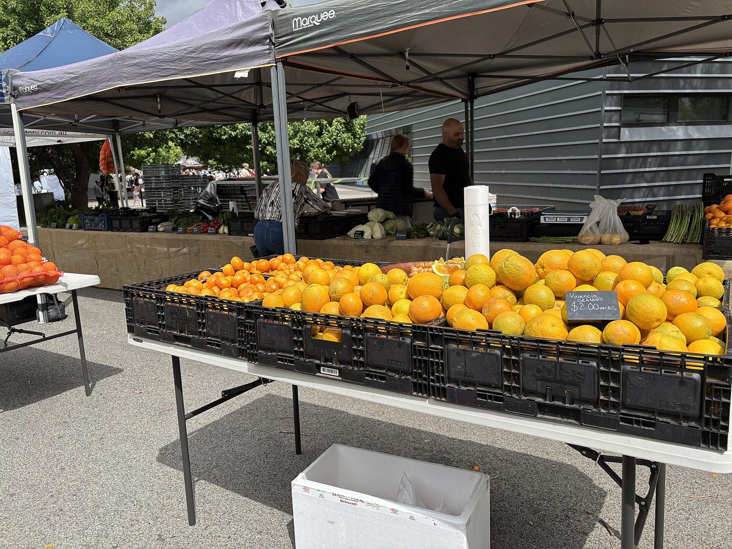
    야외 시장: 시장은 경쟁하는 용도 사이에서 희귀 자원을 배분합니다
    야외 시장: 시장은 경쟁하는 용도 사이에서 희귀 자원을 배분합니다

    경제학은 하나의 견고한 사실에서 시작됩니다: 사람들의 욕구는 사실상 무제한이지만, 그것을 충족시키는 자원은 제한되어 있다는 것입니다. 이 격차는 희귀성이며, 이것이 경제학이 존재하는 이유입니다 – 모든 것이 무료로 무제한이라면 결정할 것 자체가 없었을 것입니다.

    자원(생산 요소)은 토지(자연 자원), 노동(인간 노력), 자본(도구, 기계, 건물), 그리고 기업가정신(나머지 세 가지를 조직하고 위험을 감당함)입니다. 이들이 희귀하므로 모든 경제체는 세 가지 질문에 답해야 합니다: 무엇을, 어떻게, 누구를 위해 생산할 것인가.

    희소성으로 인해 선택이 강제되며, 모든 선택에는 기회비용이 수반됩니다. 기회비용은 포기하게 되는 차선책의 가치입니다. 이 하나의 개념이 전체 과정을 관통합니다: 어떤 것의 진정한 비용은 그것을 얻기 위해 sacrifices하는 것이지, 단순히 지불한 돈이 아닙니다.

    Vocabulary · ⁨어휘⁩ Train · ⁨연습하기⁩
    English 한국어
    Economics/ˌiːkəˈnɒmɪks/ 경제학
    resources/rɪˈzɔːsɪz/ 자원
    scarcity/ˈskeəsɪti/ 희소성
    factors of production/ˈfæktəz ɒv prəˈdʌkʃn/ 생산 요인
    labor/ˈleɪbə/ 노동
    capital/ˈkæpɪtl/ 자본
    entrepreneurship/ˌɒntrɪprəˈnjʊəʃɪp/ Entrepreneurship
    opportunity cost/ɒpəˈtjuːnɪti kɒst/ 기회비용
    1.2

    Resource Allocation and Economic Systems · ⁨자원 배분과 경제 체계⁩

    Syllabus
    English

    Enduring Understanding (MKT-1): Most resources are scarce, and in most cases the use of resources involves constraints and trade-offs.

    Learning Objective MKT-1.B: Define how resource allocation is influenced by the economic system adopted by society.

    • MKT-1.B.1 Resource allocation involves answering three basic questions: What goods and services to produce? How to produce those goods and services? And who consumes those goods and services?
    • MKT-1.B.2 Resource allocation is significantly influenced by the economic system adopted by society, such as command economy, market economy, or mixed economy. Each system involves a particular set of institutional arrangements and a coordinating mechanism for allocating scarce resources and distributing output.
    한국어

    지속적 이해 (MKT-1): 대부분의 자원은 희소하며, 대개 자원의 사용에는 제약과交換(trade-offs)이 수반된다.

    학습 목표 MKT-1.B: 사회가 채택한 경제 체제가 자원 배분에 미치는 영향을 정의하시오.

    • MKT-1.B.1 자원 배분은 다음 세 가지 기본 질문에 답하는 것을 포함한다: 어떤 재화와 서비스를 생산할 것인가? 그 재화와 서비스를 어떻게 생산할 것인가? 그리고 누가那些 재화와 서비스를 소비할 것인가?
    • MKT-1.B.2 자원 배분은 사회가 채택한 경제 체제, 즉 계획경제, 시장경제, 혹은 혼합경제에 따라 크게 달라진다. 각 체제는 희소한 자원을 배분하고 산출물을 분배하기 위해 특정의 제도적 배치와 조율 메커니즘을 포함한다.

    Source: College Board AP Course and Exam Description · ⁨출처: College Board AP Course and Exam Description⁩

    English

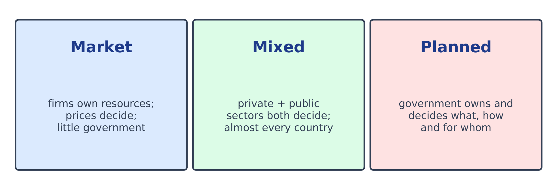
    An economic system 经济体制 is a society's way of answering the three questions.

    • In a market economy 市场经济, private buyers and sellers decide through prices; self-interest and competition coordinate them (the "invisible hand").
    • In a command economy 计划经济, the government owns resources and plans production.
    • Real economies are mixed 混合经济 – mostly markets, with government providing some goods and correcting problems.

    The key advantage of markets is that prices carry information and incentives 激励 automatically, with no central planner needed.

    한국어

    경제 체계란 사회가 세 가지 질문(무엇을, 어떻게, 누구를 위해 생산할 것인가)에 답하는 방식입니다.

    경제 체제는 자유 시장부터 완전한 정부 계획까지 스펙트럼을 형성함
    경제 체제는 자유 시장부터 완전한 정부 계획까지 스펙트럼을 형성합니다
    • 시장 경제에서는 사적 구매자와 판매자가 가격을 통해 결정하며, 이기심과 경쟁이 이를 조율합니다 ("보이지 않는 손").
    • 계획 경제에서는 정부가 자원을 소유하고 생산을 계획합니다.
    • 실제 경제는 혼합형입니다. 대부분 시장이지만, 정부가 일부 재화를 제공하고 문제를 수정합니다.

    시장의 핵심적인 장점은 가격이 정보를 내재하고 있으며 유인을 자동으로 제공하여 중앙 계획자가 필요 없다는 점입니다.

    Explore · ⁨탐색하기⁩

    Explore how prices coordinate a market · ⁨가격이 시장을 조정하는 방식 탐구하기⁩

    In a market economy no one is in charge, yet the price finds the level where quantity supplied meets quantity demanded. Drag the demand and supply lines and watch the equilibrium price act as a signal and an incentive. · ⁨시장경제에서는 주체자가 없으나, 가격은 공급량과 수요량이 일치하는 수준을 찾습니다. 수요 및 공급 곡선을 드래그하여 균형 가격이 신호이자 유인으로서 작용하는 것을 확인하십시오.⁩

    Vocabulary · ⁨어휘⁩ Train · ⁨연습하기⁩
    English 한국어
    economic system/ˌiːkəˈnɒmɪk ˈsɪstəm/ 경제 체제
    market economy/ˈmɑːkɪt ɪˈkɒnəmi/ 시장 경제
    command economy/kəˈmænd ɪˈkɒnəmi/ 지명 경제
    mixed/mɪkst/ 혼합됨
    incentives/ɪnˈsentɪvz/ 인센티브
    production possibilities curve (PPC)/prəˈdʌkʃn ˌpɒsəˈbɪlɪtiz kɜːv/ 생산 가능성 곡선 (PPC)
    efficient/ɪˈfɪʃənt/ 효율적
    unattainable/ʌnəˈteɪnəbl/ 달성 불가능하다
    Economic growth/ˌiːkəˈnɒmɪk ɡrəʊθ/ 경제 성장
    specializing/ˈspeʃəlaɪzɪŋ/ 전문화
    absolute advantage/ˈæbsəluːt ədˈvæntɪdʒ/ 절대 우위
    1.3

    The Production Possibilities Curve · ⁨생산 가능성 곡선⁩

    Syllabus
    English

    Enduring Understanding (MKT-1): Most resources are scarce, and in most cases the use of resources involves constraints and trade-offs.

    Learning Objective MKT-1.C: a. Define (using graphs as appropriate) the production possibilities curve (PPC) and related terms. b. Explain (using graphs as appropriate) how the production possibilities curve (PPC) illustrates opportunity costs, trade-offs, inefficiency, efficiency, and economic growth or contraction under various conditions. c. Calculate (using data from PPCs or tables as appropriate) opportunity cost.

    • MKT-1.C.1 The PPC is a model used to show the trade-offs associated with allocating resources.
    • MKT-1.C.2 The PPC can be used to illustrate the concepts of scarcity, opportunity cost, efficiency, underutilized resources, and economic growth or contraction.
    • MKT-1.C.3 The shape of the PPC depends on whether opportunity costs are constant, increasing, or decreasing.
    • MKT-1.C.4 The PPC can shift due to changes in factors of production as well as changes in productivity/technology.
    • MKT-1.C.5 Economic growth results in an outward shift of the PPC.
    한국어

    지속적 이해 (MKT-1): 대부분의 자원은 희소하며, 대개 자원의 사용에는 제약과交換(trade-offs)이 수반된다.

    학습목표 MKT-1.C: a. (적절한 경우 그래프를 사용하여) 생산가능곡선(PPC)과 관련 용어를 정의하시오. b. (적절한 경우 그래프를 사용하여) 생산가능곡선(PPC)이 어떤 조건 하에서 기회비용, 타협, 비효율성, 효율성, 그리고 경제 성장 또는 침체를 어떻게 나타내는지 설명하시오. c.的机会 비용을 계산하십시오(적절한 경우 PPC 또는 표의 데이터 사용).

    • MKT-1.C.1 PPC는 자원을 배분하는 데 수반되는 타협을 보여주는 모델이다.
    • MKT-1.C.2 PPC는 희소성, 기회비용, 효율성, 비활용된 자원, 그리고 경제 성장 또는 침체의 개념을 설명하는 데 사용될 수 있다.
    • MKT-1.C.3 PPC의 형태는 기회비용이 일정하게 유지되는지, 증가하는지, 감소하는지에 따라 달라진다.
    • MKT-1.C.4 생산요소의 변화 및 생산성/기술의 변화에 따라 PPC가 이동할 수 있다.
    • MKT-1.C.5 경제 성장은 PPC의 외부로 이동으로 나타난다.

    Source: College Board AP Course and Exam Description · ⁨출처: College Board AP Course and Exam Description⁩

    English
    The production possibility frontier

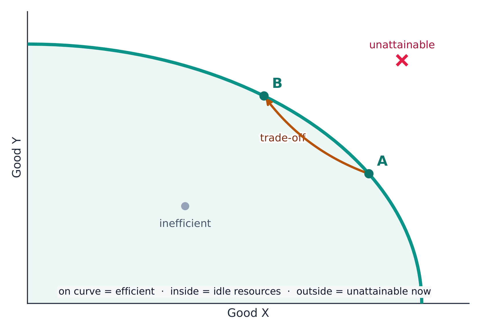
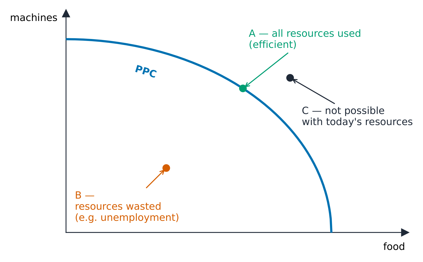
    The production possibilities curve (PPC) 生产可能性曲线 shows the maximum combinations of two goods an economy can produce with its resources and technology fully and efficiently used.

    • Points on the curve are efficient 有效率; points inside are inefficient (wasted or unemployed resources); points outside are currently unattainable 无法实现.
    • The PPC's downward slope shows opportunity cost: making more of one good means making less of the other. The slope at a point is the opportunity cost of the good on the horizontal axis.
    • A bowed-out (concave) PPC shows increasing opportunity cost – resources are not equally suited to both goods, so making more of one costs ever more of the other. A straight-line PPC means constant opportunity cost.
    • Economic growth 经济增长 (more resources, better technology) shifts the whole curve outward.

    Exam skill: be ready to read opportunity cost off a PPC, decide if a point is efficient/inefficient/unattainable, and explain what shifts the curve.

    한국어
    생산가능 Frontier

    생산 가능성 곡선(PPC) 은 경제가 자원과 기술을 완전히 및 효율적으로 활용할 때 두 재화의 최대 조합을 보여줍니다.

    생산 가능성 곡선 위의 점, 내부의 점, 외부의 점
    생산 가능성 곡선 위의 점, 내부의 점, 외부의 점
    • 곡선 위의 점은 효율적이고, 곡선 안쪽의 점은 비효율적입니다(자원이 낭비되었거나 실업 상태임); 곡선 바깥의 점은 현재로써 달성 불가능합니다.
    • PPC의 하향 경사는 기회비용을 나타냅니다: 한 재화의 생산량을 늘리면 다른 재화의 생산량은 줄어듭니다. 특정 지점에서의 기울기는 수평축에 있는 재화의 기회비용입니다.
    • 바깥쪽으로 볼록한(오목한) PPC는 증가하는 기회비용을 의미합니다. 자원은 두 재화 모두에 동등하게 적합하지 않으므로, 한 재화의 생산량이 늘어날수록 다른 재화의 생산량 감소분이 커집니다. 직선형 PPC는 일정한 기회비용을 의미합니다.
    • 경제 성장(자원 증가, 기술 발전)은 곡선 전체를 바깥쪽으로 이동시킵니다.

    고사 기법: PPC에서 기회비용을 읽거나, 점이 효율적/비효율적/달성 불가능한지를 판단하거나, 곡선을 이동시키는 요인을 설명할 수 있어야 합니다.

    생산 가능성 곡선: 효율적, 비효율적, 달성 불가능한 점
    생산 가능성 곡선: 효율적, 비효율적, 달성 불가능한 점
    Explore · ⁨탐색하기⁩

    Explore the production possibilities curve · ⁨생산 가능 곡선을 탐색해 보십시오⁩

    Making more of one good means giving up some of the other — that trade-off is the opportunity cost, and the bowed shape shows the law of increasing opportunity cost. Drag along the curve, then grow the economy to push the whole frontier out. · ⁨한 재화의 생산을 늘리면 다른 재화의 일부를 포기해야 합니다. 이 타협은 기회비용이며, 오목한 형태는 기회비용 증가의 법칙을 보여줍니다. 곡선을 드래그하고 경제를 성장시켜 전체 frontier(전개선)를 외측으로 밀어내십시오.⁩

    1.4

    Comparative Advantage and Gains from Trade · ⁨비교 우위 및 무역의 이점⁩

    Syllabus
    English

    Enduring Understanding (MKT-2): The consequences of scarcity can be mitigated through specialization in production and by exchange.

    Learning Objective MKT-2.A: a. Define absolute advantage and comparative advantage. b. Determine (using data from PPCs or tables as appropriate) absolute and comparative advantage.

    • MKT-2.A.1 Absolute advantage describes a situation in which an individual, business, or country can produce more of a good or service than any other producer with the same quantity of resources.
    • MKT-2.A.2 Comparative advantage describes a situation in which an individual, business, or country can produce a good or service at a lower opportunity cost than another producer.

    Learning Objective MKT-2.B: a. Explain (using data from PPCs or tables as appropriate) how specialization according to comparative advantage with appropriate terms of trade can lead to gains from trade. b. Calculate (using data from PPCs or tables as appropriate) mutually beneficial terms of trade.

    • MKT-2.B.1 Production specialization according to comparative advantage, not absolute advantage, results in exchange opportunities that lead to consumption possibilities beyond the PPC.
    • MKT-2.B.2 Comparative advantage and opportunity costs determine the terms of trade for exchange under which mutually beneficial trade can occur.
    한국어

    지속적 이해 (MKT-2): 희소성의 결과들은 생산에서의 전문화와 교환을 통해 완화될 수 있다.

    학습 목표 MKT-2.A: a. 절대 우위와 비교 우위를 정의하십시오. b. 절대 우위와 비교 우위를 결정하십시오(적절한 경우 PPC 또는 표의 데이터 사용).

    • MKT-2.A.1 절대 우위는 개인, 기업, 혹은 국가가 동일한 양의 자원으로 다른 모든 생산자보다 더 많은 재화나 서비스를 생산할 수 있는 상황을 말한다.
    • MKT-2.A.2 비교 우위는 개인, 기업, 혹은 국가가 다른 생산자보다 낮은 기회비용으로 재화나 서비스를 생산할 수 있는 상황을 말한다.

    학습목표 MKT-2.B: a. 비교 우위에 따른 전문화와 적절한 거래 조건이 거래 이득으로 이어지는 방법을 설명하십시오(적절한 경우 PPC 또는 표의 데이터 사용). b. 상호 유익한 거래 조건을 계산하십시오(적절한 경우 PPC 또는 표의 데이터 사용).

    • MKT-2.B.1 절대 우위가 아닌 비교 우위에 따른 생산 전문화는 생산가능곡선(PPC)을 넘어선 소비 가능성을 제공하는 교환 기회를 창출한다.
    • MKT-2.B.2 비교 우위와 기회비용은 서로에게 유익한 무역이 이루어질 수 있는 교환의 조건을 결정한다.

    Source: College Board AP Course and Exam Description · ⁨출처: College Board AP Course and Exam Description⁩

    English

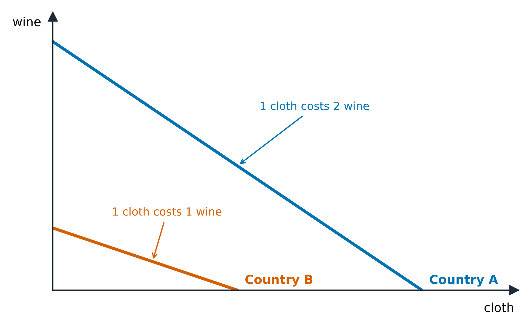
    Two producers can both gain from trade by specializing 专业化.

    • A producer has an absolute advantage 绝对优势 in a good if it can make more of it with the same resources.
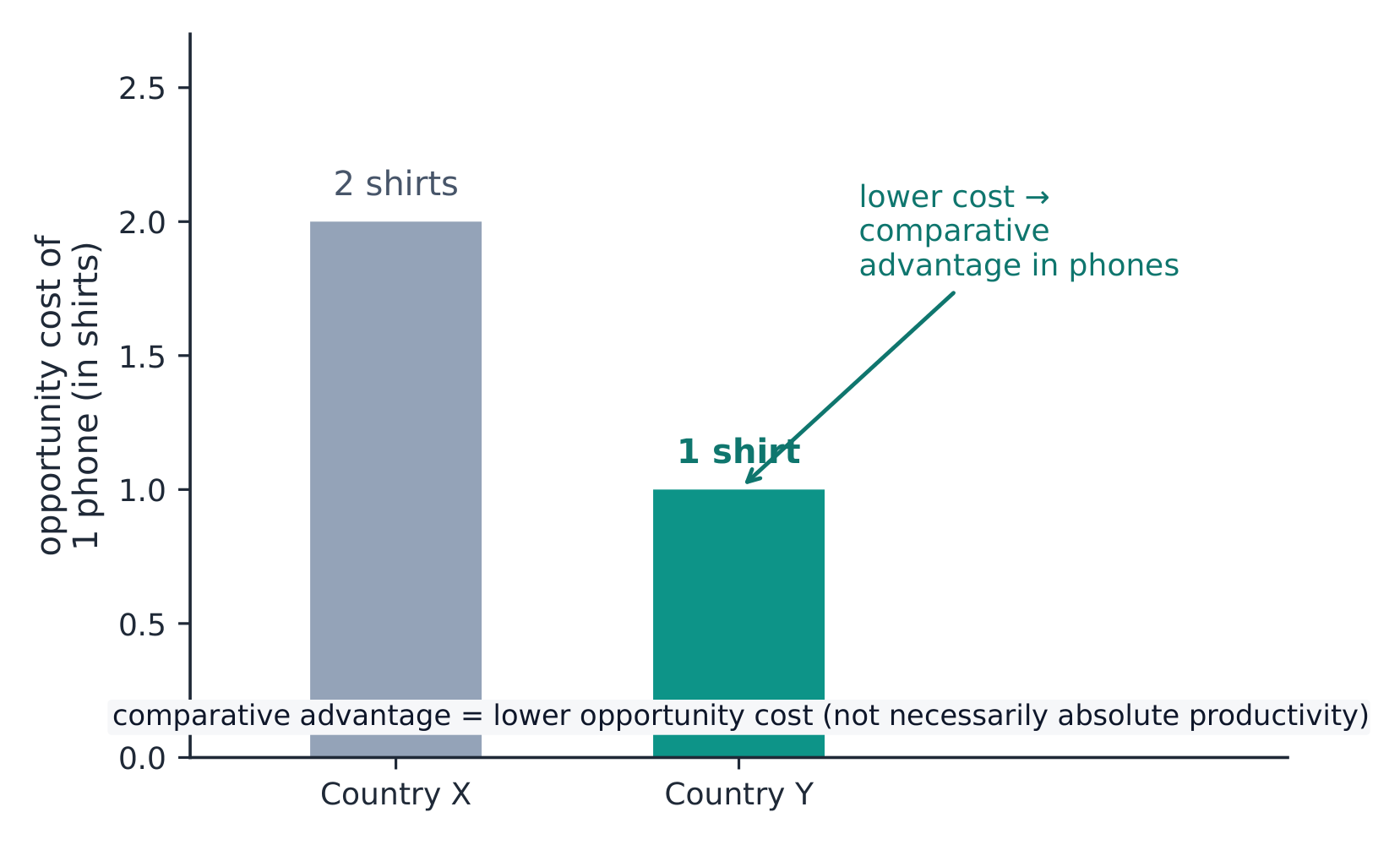
    • A producer has a comparative advantage 比较优势 if it has the lower opportunity cost for that good. Comparative advantage – not absolute – determines who should specialize.
    • Compute opportunity cost from output data: for each producer, one unit of good X costs (units of Y) $\div$ (units of X). The producer who gives up less Y should make X.
    • Both sides gain if they trade at a rate between their two opportunity costs – the terms of trade 贸易条件. Specializing by comparative advantage lets total output exceed what either could make alone, so consumption can lie outside each producer's own PPC.

    Worked example. Anna can make $20$ shirts or $10$ tables a day; Ben can make $12$ shirts or $12$ tables. For Anna one table costs $\tfrac{20}{10}=2$ shirts; for Ben it costs $\tfrac{12}{12}=1$ shirt. Ben gives up fewer shirts, so Ben specializes in tables and Anna in shirts. Any terms of trade between $1$ and $2$ shirts per table – say $1.5$ – leaves both better off than producing alone.

    Exam skill: these calculations appear almost every year – practice finding comparative advantage from both output tables and input tables, and stating a valid terms-of-trade range.

    한국어

    두 생산자가 전문화(specialization) 를 통해 교역으로부터 모두 이득을 얻을 수 있습니다.

    비교 우위는 기울기가 다른 생산 가능 곡선에서 비롯됩니다
    비교 우위는 기울기가 다른 생산 가능 곡선에서 비롯됩니다
    • 한 생산자가 동일한 자원으로 더 많은 양을 생산할 수 있을 때, 그 재화에 대해 절대 우위를 가집니다.
    • 한 생산자가 해당 재화에 대해 더 낮은 기회비용을 가질 때, 비교 우위를 가집니다. 절대 우위가 아니라 비교 우위가 누가 전문화해야 할지를 결정합니다.
    • 산출 데이터로부터 기회비용을 계산합니다: 각 생산자에 대해 재화 X 1단위의 비용은 Y 단位数 $\div$ ÷ X 단位数 (units of X)입니다. 더 적은 Y를 포기하는 생산자가 X를 생산해야 합니다.
    • 양측이 서로의 기회비용 사이의 비율로 교역할 때(이를 교역 조건이라 함), 모두 이득을 봅니다. 비교 우위에 따른 전문화는 총 산출량을 개별 생산자가 단독으로 생산할 수 있는 것을 초과하게 하므로, 소비는 각 생산자의 own PPC 바깥에 위치할 수 있습니다.

    해설 예제. 안나는 하루에 $20$개의 셔츠 또는 $10$개의 테이블을 만들 수 있고, 벤은 하루에 $12$개의 셔츠 또는 $12$개의 테이블을 만들 수 있습니다. 안나에게 테이블 1개는 $\tfrac{20}{10}=2$개의 셔츠를 의미하고, 벤에게는 $\tfrac{12}{12}=1$개의 셔츠를 의미합니다. 벤이 더 적은 셔츠를 포기하므로 벤은 테이블에 전문화하고 안나는 셔츠에 전문화합니다. 테이블당 $1$개와 $2$개 사이의 어떤 교역 조건 – 예를 들어 $1.5$개 – 이라면 두 사람 모두 단독 생산보다 나아집니다.

    고사 기법: 이러한 계산은 거의 매년 출제되므로, 산출표와 투입표 모두에서 비교 우위를 찾고 유효한 교역 조건 범위를 서술하는 연습을 하십시오.

    비교 우위는 기회 비용이 낮은 생산자에게 배당됩니다
    비교 우위는 더 낮은 기회비용을 가진 생산자에게 돌아갑니다
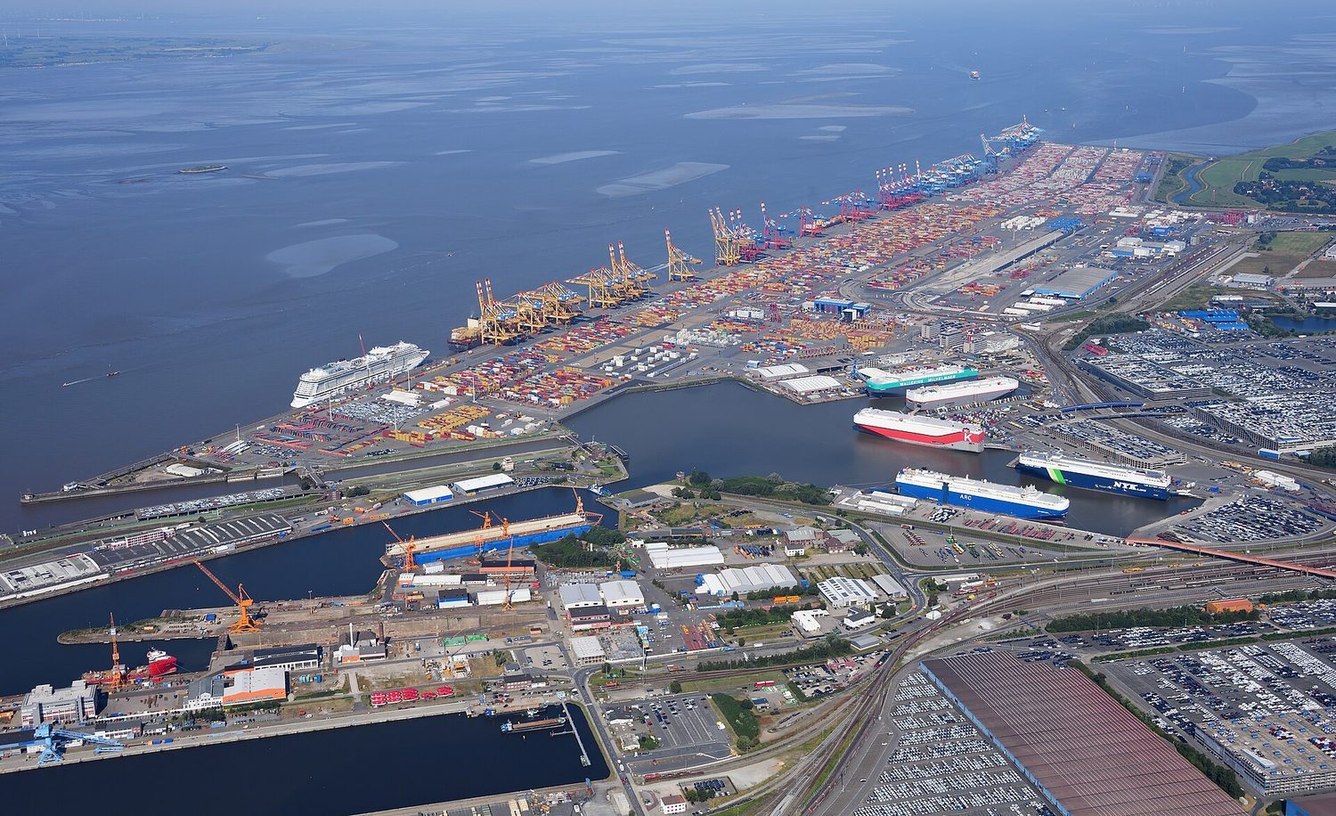
    컨테이너 운송: 비교 우위와 무역은 국가의 전문화와 이득을 가능하게 합니다
    컨테이너 운송: 비교 우위와 무역은 국가의 전문화와 이득을 가능하게 합니다
    Explore · ⁨탐색하기⁩

    See why trade lets you consume beyond the frontier · ⁨무역이 frontier(전개선) 너머 소비를 가능하게 하는 이유 보기⁩

    A producer should specialize where its opportunity cost is lowest, then trade for the rest. Because the terms of trade lie between the two producers' costs, trade lets a country consume outside its own production frontier. · ⁨생산자는 기회비용이 가장 낮은 곳에서 전문화하고 나머지는 무역을 통해 조달해야 합니다. 무역 조건이 두 생산자의 비용 사이에 있으므로, 무역은 국가가 자체 생산 frontier(전개선) 바깥에서 소비할 수 있게 합니다.⁩

    Vocabulary · ⁨어휘⁩ Train · ⁨연습하기⁩
    English 한국어
    comparative advantage/kəmˈpærətɪv ədˈvæntɪdʒ/ 상대적 우위
    terms of trade/tɜːmz ɒv treɪd/ Terms of Trade
    1.5

    Cost-Benefit Analysis · ⁨비용-편익 분석⁩

    Syllabus
    English

    Enduring Understanding (CBA-1): Rational economic decisions require the evaluation of costs and benefits.

    Learning Objective CBA-1.A: a. Define opportunity cost. b. Explain the opportunity costs associated with choices. c. Calculate the opportunity costs associated with choices.

    • CBA-1.A.1 Rational agents consider opportunity costs, whether implicit or explicit, when calculating the total economic costs of any decision.
    • CBA-1.A.2 Total benefits form the metric "utility" for consumers and total revenue for firms.

    Learning Objective CBA-1.B: a. Explain a decision by comparing total benefits and total costs (using a table or a graph when appropriate). b. Calculate total benefits and total costs (using a table or graph where appropriate).

    • CBA-1.B.1 Total net benefits, the difference between total benefits and total costs, are maximized at the optimal choice.
    • CBA-1.B.2 Some decisions permit rational agents to look at only marginal benefit and marginal cost. Other decisions cannot be broken down into increments in this way and must be evaluated by looking at total benefits and total costs.
    한국어

    지속적 이해 (CBA-1): 합리적인 경제 결정은 비용과 편익의 평가가 요구된다.

    학습목표 CBA-1.A: a. 기회비용을 정의하시오. b. 선택에 수반되는 기회비용을 설명하시오. c. 선택에 수반되는 기회비용을 계산하시오.

    • CBA-1.A.1 합리적 주체는 어떤 결정에 대한 총 경제 비용을 계산할 때 암묵적이든 명시적이든 기회비용을 고려한다.
    • CBA-1.A.2 총 편익은 소비자에게는 '편익'이라는 지표가 되며 기업에게는 총 매출이 된다.

    학습목표 CBA-1.B: a. (적절한 경우 표나 그래프를 사용하여) 총 편익과 총 비용을 비교하여 결정을 설명하시오. b. (적절한 경우 표나 그래프를 사용하여) 총 편익과 총 비용을 계산하시오.

    • CBA-1.B.1 총 편익과 총 비용의 차이인 순총 편익은 최적의 선택 지점에서 최대화된다.
    • CBA-1.B.2 일부 결정은 합리적 주체가 한계 편익과 한계 비용만 보게允许한다. 다른 결정들은 이的方式로 세분할 수 없으며, 총 편익과 총 비용을 살펴서 평가되어야 한다.

    Source: College Board AP Course and Exam Description · ⁨출처: College Board AP Course and Exam Description⁩

    English

    Rational decision-makers weigh benefits against costs. An action is worthwhile only when its benefit is at least as large as its cost – including the opportunity cost. Money already spent and unrecoverable is a sunk cost 沉没成本 and should be ignored in decisions: only future costs and benefits matter.

    한국어

    합리적인 의사결정자는 편익을 비용과 대조합니다. 행동의 편익이 비용 이상일 때만 그 행동은 타당합니다.这里包括机会成本。 이미 지출되어 회수할 수 없는 돈은 沉没成本이며, 의사결정 시 고려해서는 안 됩니다: 오직 미래의 비용과 편익만 중요합니다.

    Explore · ⁨탐색하기⁩

    Weigh total benefit against total cost · ⁨총편익과 총비용 비교하기⁩

    A choice is worth it only while the benefit of one more unit beats its cost. Where total revenue meets total cost is the break-even point; past it, extra activity adds more cost than value. · ⁨한 단위당 편익이 비용보다 클 때까지 택은 가치 있는 것입니다. 총수입과 총비용이 만나는 지점이 손익분기점이며, 그 이후로는 추가 활동이 가치보다 더 많은 비용을 초래합니다.⁩

    1.6

    Marginal Analysis and Consumer Choice · ⁨한계 분석과 소비자 선택⁩

    Syllabus
    English

    Enduring Understanding (CBA-2): To determine the optimal level at which to pursue an activity whose total benefits exceed total cost, rational economic agents compare marginal benefits and marginal costs.

    Learning Objective CBA-2.A: a. Define the key assumptions of consumer choice theory. b. Explain (using a table or graph as appropriate) how a rational consumer's decision making involves the use of marginal benefits and marginal costs. c. Calculate (using a table or a graph when appropriate) how a rational consumer's decision making involves the use of marginal benefits and marginal costs.

    • CBA-2.A.1 Consumers face constraints and have to make optimal decisions accounting for these constraints.
    • CBA-2.A.2 In a model of rational consumer choice, consumers are assumed to make choices so as to maximize their total utility.
    • CBA-2.A.3 Consumers experience diminishing marginal utility in the consumption of goods and services.
    • CBA-2.A.4 Consumers allocate their limited income to purchase the combination of goods that maximizes their utility by equating/comparing the marginal utility of the last dollar spent on each good.
      • Exclusion statement: Indifference curves are beyond the scope of the course and the AP Exam, but equating the ratios of marginal utility to price is within the scope.

    Learning Objective CBA-2.B: a. Define marginal analysis and related terms. b. Explain a decision using marginal analysis (using a table or a graph when appropriate).

    • CBA-2.B.1 Marginal analysis involves comparing the additional benefit of increasing a given activity with the additional cost. Comparing marginal benefit (MB) with marginal cost (MC) helps individuals (firms) decide whether to increase, decrease, or maintain their consumption (production) levels.
    • CBA-2.B.2 The optimal quantity at any point in time does not depend on fixed costs (sunk costs) or fixed benefits that have already been determined by past choices.
    • CBA-2.B.3 The optimal quantity is achieved when marginal benefit is equal to marginal cost or where total benefit is maximized.
    한국어

    지속적 이해 (CBA-2): 총 편익이 총 비용 초과일 때 어떤 활동을 추구할 최적 수준을 결정하기 위해 합리적 경제 주체는 한계 편익과 한계 비용을 비교한다.

    학습목표 CBA-2.A: a. 소비자 선택 이론의 핵심 가정들을 정의하시오. b. (적절한 경우 표나 그래프를 사용하여) 합리적 소비자의 의사결정이 한계 편익과 한계 비용의 활용을 어떻게 포함하는지 설명하시오. c. (적절한 경우 표나 그래프를 사용하여) 합리적 소비자의 의사결정이 한계 편익과 한계 비용의 활용을 어떻게 포함하는지 계산하시오.

    • CBA-2.A.1 소비자는 제약을 faced하며, 이러한 제약을 고려하여 최적의 결정을 내린다.
    • CBA-2.A.2 합리적 소비자 선택 모델에서 소비자는 총 편익을 극대화하도록 선택한다고 가정한다.
    • CBA-2.A.3 소비자는 재화와 서비스 소비 시递减한 한계 편익을 경험한다.
    • CBA-2.A.4 소비자는 제한된 소득을 각 재화에_last dollar에 대한 한계 편익을 동일하게 하거나 비교함으로써 편익을 극대화하는 재화의 조합에 할당한다.
      • 제외 문구: 무차별 곡선은 과정 및 AP 시험 범위를 벗어나지만, 한계 편익과 가격의 비율을 동일하게 하는 것은 범위 내에 포함된다.

    학습목표 CBA-2.B: a. 한계 분석과 관련 용어를 정의하시오. b. (적절한 경우 표나 그래프를 사용하여) 한계 분석을 사용하여 결정을 설명하시오.

    • CBA-2.B.1 한계 분석은给定 활동의 증가는 추가 편익과 추가 비용을 비교하는 것을 포함한다. 한계 편익(MB)을 한계 비용(MC)과 비교하면 개인(기업)이 소비(생산) 수준을 증가, 감소, 혹은 유지해야 할지 결정하는 데 도움이 된다.
    • CBA-2.B.2 어떤 시점에서의 최적 수량은 과거 선택에 의해 이미 결정된 고정비(沉没成本)나 고정편익에 의존하지 않는다.
    • CBA-2.B.3 최적 수량은 한계 편익이 한계 비용과 같아지거나 총 편익이 최대화되는 지점에서 달성된다.

    Source: College Board AP Course and Exam Description · ⁨출처: College Board AP Course and Exam Description⁩

    English

    Most real decisions are not "all or nothing" but "a little more or a little less." Marginal analysis 边际分析 compares the marginal benefit 边际收益 (the benefit of one more unit) with the marginal cost 边际成本 (the cost of one more unit).

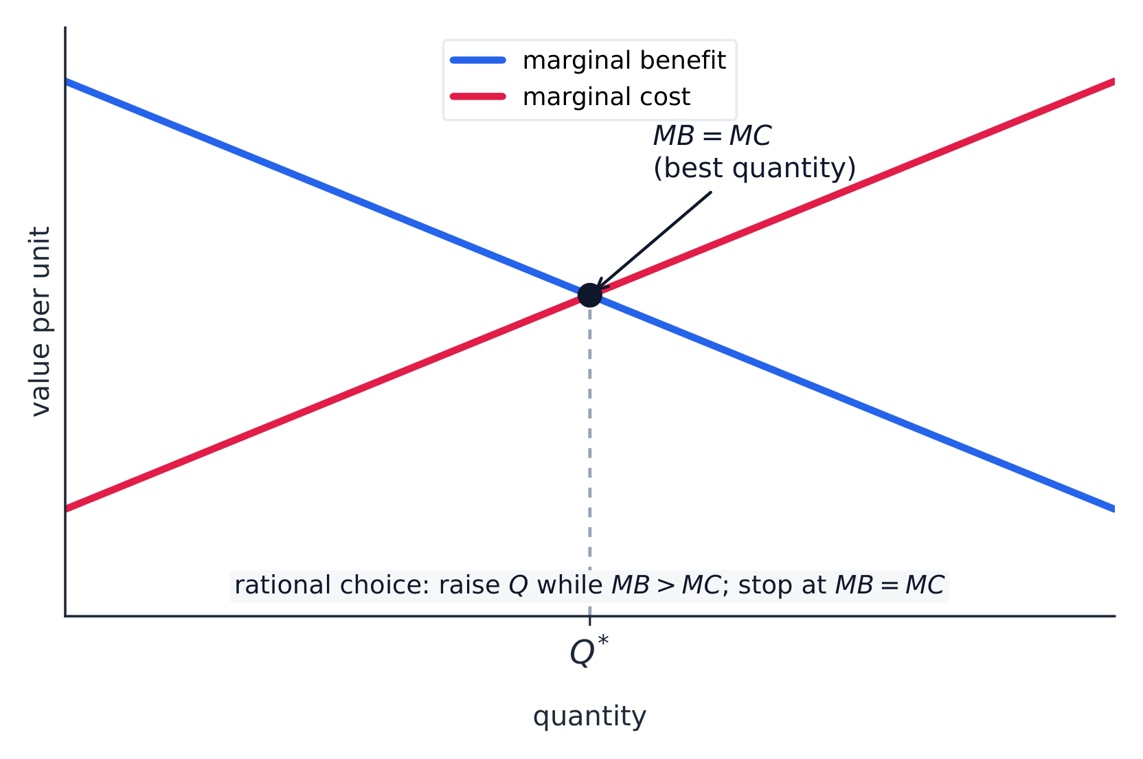
    • Decision rule: keep doing the activity while marginal benefit $>$ marginal cost; stop where MB $=$ MC. That point maximizes net benefit (total benefit minus total cost).
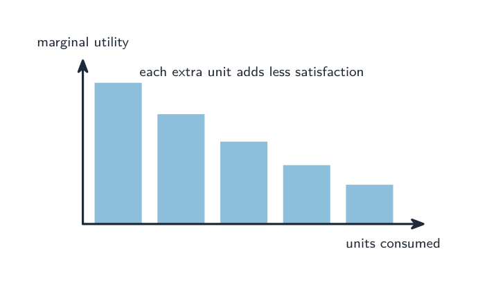
    • Consumers get utility 效用 (satisfaction) from goods, but each extra unit usually gives less added satisfaction – the law of diminishing marginal utility 边际效用递减法则.
    • A consumer maximizes total utility by the utility-maximizing rule: spend so that the marginal utility per dollar is equal across all goods, $\dfrac{MU_x}{P_x}=\dfrac{MU_y}{P_y}$, using up the whole budget. If one good gives more utility per dollar, buy more of it until the ratios equalize.

    Worked example. A consumer is choosing between good X ($MU_x=20$, $P_x=\$2$) and good Y ($MU_y=15$, $P_y=\$1$). The utility per dollar is $\tfrac{20}{2}=10$ for X but $\tfrac{15}{1}=15$ for Y. Y delivers more satisfaction per dollar, so the consumer should buy more Y and less X; as they do, $MU_y$ falls and $MU_x$ rises until $\tfrac{MU_x}{2}=\tfrac{MU_y}{1}$ and the budget is spent.

    Exam skill: the "MB = MC" logic and the "equal MU-per-dollar" rule are tested repeatedly – be able to find the optimal quantity from a table and explain why it is optimal.

    한국어

    실제 대부분의 의사결정은 "모두 또는 아무것도"가 아니라 "약간 더 많거나 적게"입니다. 한계 분석은 한계 편익(추가 1단위의 편익)과 한계 비용(추가 1단위의 비용)을 비교합니다.

    소비되는 추가 단위마다 추가 만족도가 감소함(한계效用递减)
    소비되는 추가 단위마다 추가 만족도가 감소함(한계效用递减)
    • 결정 규칙: 한계 편익 $>$ 한계 비용인 동안 활동을 계속하고, MB $=$ MC 지점에서 중단합니다. 이 점은 순편익(총편익 minus 총비용)을 극대화합니다.
    • 소비자는 재화에서 효용(만족도)을 얻지만, 일반적으로 추가 단위는 더 적은 추가 만족도를 제공합니다 – 이는 한계 효용 체감의 법칙입니다.
    • 소비자는 유틸리티 극대화 규칙에 따라 총 유틸리티를 극대화합니다: 모든 재화에서 달러당 한계效用이 동일하도록, 즉 $\dfrac{MU_x}{P_x}=\dfrac{MU_y}{P_y}$, 전체 예산을 소진하도록 지출합니다. 한 재화가 달러당 더 높은 유틸리티를 제공하면, 비율이 일치할 때까지 그 재화를 더 많이 구매합니다.

    해설 예제. 소비자가 재화 X($MU_x=20$, $P_x=\$2$) and good Y ($MU_y=15$, $P_y=\$1$)와 재화 Y 사이에서 선택하고 있습니다. 달러당 유틸리티는 X의 경우 $\tfrac{20}{2}=10$이지만 Y의 경우 $\tfrac{15}{1}=15$입니다. Y가 달러당 더 많은 만족도를 제공하므로 소비자는 Y를 더 많이, X를 적게 구매해야 합니다.这样做时, $MU_y$이 감소하고 $MU_x$이 상승하여 $\tfrac{MU_x}{2}=\tfrac{MU_y}{1}$가 되고 예산이 소진됩니다.

    고사 기법: "MB = MC" 논리와 "달러당 한계效用 등가" 규칙은 반복해서 출제됩니다. 표에서 최적 수량을 찾고 왜 그것이 최적인지 설명할 수 있어야 합니다.

    합리적 선택: 한계편익이 한계비용을 초과할 때까지 계속하고, 두 값이 같아지는 지점에서 멈춘다
    합리적 선택: 한계편익이 한계비용을 초과할 때까지 계속하고, 두 값이 같아지는 지점에서 멈춘다
    Vocabulary · ⁨어휘⁩ Train · ⁨연습하기⁩
    English 한국어
    utility/juːˈtɪlɪti/ 유틸리티/utility
    law of diminishing marginal utility/lɔː ɒv dɪˈmɪnɪʃɪŋ ˈmɑːdʒɪnl juːˈtɪlɪti/ 한계 효용 체감의 법칙
    1.6

    Exam tips · ⁨시험 팁⁩

    English
    • Opportunity cost is the next-best alternative given up; ignore sunk costs in any decision.
    • Comparative advantage (lower opportunity cost) determines specialisation and the gains from trade.
    • Apply marginal analysis: keep doing an activity while MB > MC, stopping where MB = MC.
    • Maximise utility by equalising the marginal utility per dollar across goods.
    • Read opportunity cost off the PPC slope; a bowed curve shows increasing cost.
    한국어
    • 기회비용은 포기한 차선책의 대가이며, **沉没原費( sunk costs)**는 모든 의사결정에서 고려하지 않아야 한다.
    • 비교우위(더 낮은 기회비용)는 전문화와 무역의 이점을 결정한다.
    • 한계분석을 적용하라: MB > MC일 때 해당 활동을 유지하고, MB = MC가 되는 지점에서 멈추라.
    • 재화 간 달러당 한계효용을 동일하게 하여 효용을 극대화하라.
    • PPC의 기울기에서 기회비용을 읽으라. 오목한 곡선은 증가하는 비용을 의미한다.
    Vocabulary · ⁨어휘⁩ Train · ⁨연습하기⁩
    English 한국어
    sunk cost/sʌŋk kɒst/ 沉没成本
    Marginal analysis/ˈmɑːdʒɪnl əˈnæləsɪs/ 한계 분석
    marginal benefit/ˈmɑːdʒɪnl ˈbenɪfɪt/ 한계 편익
    marginal cost/ˈmɑːdʒɪnl kɒst/ 한계비용
  • 2

    Supply and Demand · ⁨공급과 수요⁩

    Watch lesson · ⁨수업 보기⁩
    2.1

    Demand · ⁨수요⁩

    Syllabus
    English

    Enduring Understanding (MKT-3): Individuals and firms respond to incentives and face constraints.

    Learning Objective MKT-3.A: a. Define (using graphs as appropriate) key terms and factors related to consumer decision making and the law of demand. b. Explain (using graphs as appropriate) the relationship between price and quantity demanded and how buyers respond to incentives and constraints.

    • MKT-3.A.1 A well-defined system of property rights is necessary for the market system to function well.
    • MKT-3.A.2 Economic agents respond to incentives.
    • MKT-3.A.3 Individuals often respond to incentives, such as those presented by prices, but also face constraints, such as income, time, and legal and regulatory frameworks.
    • MKT-3.A.4 The law of demand suggests that a change in the own-price causes a change in quantity demanded in the opposite direction and a movement along a demand (marginal benefit) curve.
    • MKT-3.A.5 The conceptual relationship between price and quantity stated by the law of demand leads to downward-sloping demand curves explained by the income effect and substitution effect and/or by diminishing marginal utility.
    • MKT-3.A.6 The market demand curve (schedule) is derived from the summation of individual demand curves (schedules).

    Learning Objective MKT-3.B: Explain (using graphs as appropriate) buyers' responses to changes in incentives and constraints.

    • MKT-3.B.1 Changes in the determinants of consumer demand can cause the demand curve to shift.
    한국어

    지속적 이해 (MKT-3): 개인과 기업은 유인에 반응하며 제약을 받는다.

    학습 목표 MKT-3.A: a. 소비자의 의사결정 및 수요의 법칙과 관련된 핵심 용어 및 요인을 정의하시오(필요시 그래프 활용). b. 가격과 수량 간 관계 및 구매자가 유인과 제약에 어떻게 반응하는지를 설명하시오(필요시 그래프 활용).

    • MKT-3.A.1 시장 체제가 원활하게 작동하기 위해서는 명확히 정의된 재산권 체계가 필요하다.
    • MKT-3.A.2 경제 주체는 유인에 반응한다.
    • MKT-3.A.3 개인은 가격과 같은 유인에 자주 반응하지만, 소득, 시간, 법적 및 규제 체계와 같은 제약을 받기도 한다.
    • MKT-3.A.4 수요의 법칙에 따르면 자가격 격의 변화는 수량에 반대 방향으로 변화를 일으키며, 이는 수요(한계 효용) 곡선 위에서의 이동을 의미한다.
    • MKT-3.A.5 수요의 법칙이 제시하는 가격과 수량의 개념적 관계는 소득 효과와 대체 효과, 그리고/또는 한계 효용 체감 원리에 의해 하향 경사需求 곡선으로 설명된다.
    • MKT-3.A.6 시장 수요 곡선(수요표)은 개별 수요 곡선(수요표)들의 합산에서 유도된다.

    학습 목표 MKT-3.B: 유인과 제약의 변화에 대한 구매자의 반응을 설명하시오(필요시 그래프 활용).

    • MKT-3.B.1 소비자의 수요를 결정하는 요인의 변화는 수요 곡선을 이동시킬 수 있다.
    Source: College Board AP Course and Exam Description · ⁨출처: College Board AP Course and Exam Description⁩

    English
    Supply & demand: a shift raises P and Q

    A market works only where property rights 产权 are well defined – owners can use, exclude others from, and trade their resources; without them, prices cannot coordinate exchange. Within that framework, the two forces are demand and supply.

    Demand 需求 is the relationship between the price of a good and the quantity buyers are willing and able to buy. The law of demand 需求定律 says price and quantity demanded move in opposite directions, so the demand curve slopes downward. Two reasons: the substitution effect 替代效应 (when a good gets pricier, buyers switch to alternatives) and the income effect 收入效应 (a higher price shrinks real purchasing power).

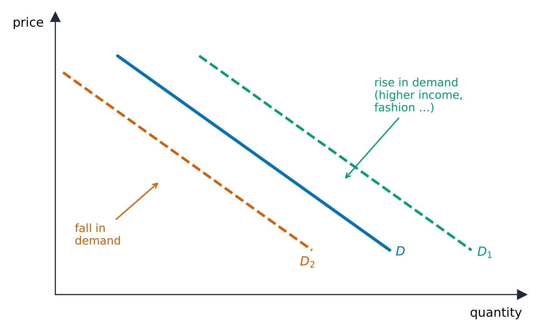
    Distinguish a change in quantity demanded (a move along the curve, caused only by the good's own price) from a change in demand (a shift of the whole curve). Demand shifts with the determinants 决定因素, remembered as TRIBE:

    • Tastes/preferences,
    • Related goods – a rise in the price of a substitute 替代品 raises demand; a rise in the price of a complement 互补品 lowers it,
    • Income – for a normal good 正常商品 more income raises demand; for an inferior good 低档商品 it lowers it,
    • Buyers (number of consumers),
    • Expectations of future price or income.

    The market demand curve is the horizontal summation 水平相加 of every individual buyer's demand curve – at each price, add up the quantities all buyers want. That is why more buyers (the B above) shifts the whole market curve to the right.

    한국어
    시장 속 쇼핑객: 수요는 수량 요구가 가격에 어떻게 반응하는지를 보여줍니다
    시장 속 구매자: 수요는 수요량이 가격에 어떻게 반응하는지를 보여준다
    공급 및 수요: 이동은 P와 Q를 높입니다

    시장은 재산권이 명확히 정의될 때만 기능한다. 소유자는 자원을 사용하거나 타인을 배제하며 거래할 수 있으며, 재산권이 없으면 가격은 교환을 조정할 수 없다. 그 틀 안에서는 두 가지 힘인 수요와 공급이 작용한다.

    수요는 재화의 가격과 구매자가 사려하고 구매할 수 있는 수량 간의 관계이다. 수요의 법칙은 가격과 수需求量가 반대 방향으로 움직이므로 수요곡선은 하향으로 경사됨을 말한다. 그 이유는 교체효과(재화가 비싸지면 구매자가 대체재로 전환함)와 소득효과(높은 가격이 실질 구매력을 감소시) 때문이다.

    수요 곡선은 아래로 경사되며, 소득, 취향, 관련 가격이 이를 이동시킵니다
    수요 곡선은 아래로 경사되며, 소득, 취향, 관련 가격이 이를 이동시킵니다

    수요량의 변화(곡선 상에서의 이동, 오직 재화의 자신 가격에 의해 발생)와 수요의 변화(전체 곡선의 이동)를 구별하라. 수요는 TRIBE라고 기억되는 요구인자에 따라 이동한다:

    • Taste/Preference(취향/선호),
    • Related goods(관련재): 대체재의 가격이 상승하면 수요가 증가하고, 보완재의 가격이 상승하면 수요가 감소함,
    • Income(소득): 정상재는 소득 증가 시 수요가 늘고, 저급재는 소득 증가 시 수요가 줄어듦,
    • Buyers(구매자: 소비자 수),
    • Expectations of future price or income(미래 가격 또는 소득에 대한 기대).

    시장수요곡선은 각 개별 구매자의 수요곡선을 수평 합산한 것이다. 모든 가격 수준에서 모든 구매자가 원하는 수량을 더하는 것이므로, 더 많은 구매자(B)가 시장 전체 곡선을 오른쪽으로 이동시킨다.

    Explore · ⁨탐색하기⁩

    Shift demand and watch price and quantity · ⁨수요를 이동시키고 가격 및 수량 확인하기⁩

    The demand curve slopes down: lower price, more wanted. A change in income, tastes or related-good prices shifts the whole curve, moving the equilibrium. · ⁨수요 곡선은 하향 사선입니다: 가격이 낮을수록 더 많이 원합니다. 소득, 취향 또는 관련재 가격의 변화는 전체 곡선을 이동시켜 균형을 바꿉니다.⁩

    Vocabulary · ⁨어휘⁩ Train · ⁨연습하기⁩
    English 한국어
    property rights/ˈprɒpəti raɪts/ 재산권
    Demand/dɪˈmænd/ 수요
    law of demand/lɔː ɒv dɪˈmænd/ 수요의 법칙
    substitution effect/ˌsʌbstɪˈtjuːʃn ɪˈfekt/ 교체 효과
    income effect/ˈɪŋkʌm ɪˈfekt/ 소득 효과 때문
    determinants/dɪˈtɜːmɪnənts/ 영향 요인(determinants)
    substitute/ˈsʌbstɪtjuːt/ 치환
    complement/ˈkɒmplɪmənt/ 보 event
    normal good/ˈnɔːml ɡʊd/ 정품
    inferior good/ɪnˈfɪərɪə ɡʊd/ 저급품
    horizontal summation/ˌhɒrɪˈzɒntl sʌˈmeɪʃn/ 수평 합계
    Supply/səˈplaɪ/ 공급
    law of supply/lɔː ɒv səˈplaɪ/ 공급의 법칙(law of supply)
    subsidies/ˈsʌbsɪdiz/ 보조금
    Price elasticity of demand/praɪs ɪlæˈstɪsɪti ɒv dɪˈmænd/ 수요의 가격 탄력성
    2.2

    Supply · ⁨공급⁩

    Syllabus
    English

    Enduring Understanding (MKT-3): Individuals and firms respond to incentives and face constraints.

    Learning Objective MKT-3.C: a. Define (using graphs as appropriate) the law of supply. b. Explain (using graphs as appropriate) the relationship between price and quantity supplied.

    • MKT-3.C.1 A change in own-price causes a change in quantity supplied in the same direction and a movement along a supply curve.
    • MKT-3.C.2 The market supply curve (schedule) is derived from the summation of individual supply curves (schedules). The market supply curve is upward-sloping.

    Learning Objective MKT-3.D: Explain (using graphs as appropriate) producers' (sellers') responses to changes in incentives and technology.

    • MKT-3.D.1 Changes in the determinants of supply can cause the supply curve to shift.
    한국어

    지속적 이해 (MKT-3): 개인과 기업은 유인에 반응하며 제약을 받는다.

    학습 목표 MKT-3.C: a. 공급의 법칙을 정의하십시오(적절한 경우 그래프 사용). b. 가격과 공급량 간의 관계를 설명하시오(필요시 그래프 활용).

    • MKT-3.C.1 자가격 격의 변화는 공급량에 같은 방향으로 변화를 일으키며, 이는 공급 곡선 위에서의 이동을 의미한다.
    • MKT-3.C.2 시장 공급 곡선(공급표)은 개별 공급 곡선(공급표)들의 합산에서 유도된다. 시장 공급 곡선은 상향 경사이다.

    학습 목표 MKT-3.D: 생산자(판매자)가 유인과 기술의 변화에 어떻게 반응하는지를 설명하시오(필요시 그래프 활용).

    • MKT-3.D.1 공급을 결정하는 요인의 변화는 공급 곡선을 이동시킬 수 있다.

    Source: College Board AP Course and Exam Description · ⁨출처: College Board AP Course and Exam Description⁩

    English
    A shift in supply

    Supply 供给 is the relationship between price and the quantity sellers will offer. The law of supply 供给定律: price and quantity supplied move in the same direction, so the supply curve slopes upward (higher prices cover higher marginal costs and reward more output).

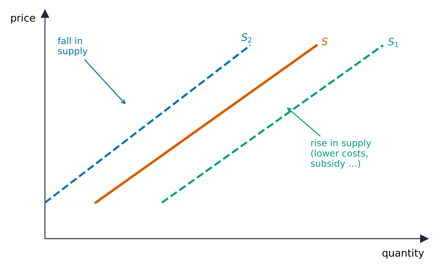
    Again separate a change in quantity supplied (movement along the curve, from the good's own price) from a change in supply (a shift). Supply shifts with input prices, technology, taxes and subsidies 补贴, prices of other goods a firm could make, number of sellers, and expectations. Just like demand, the market supply curve is the horizontal sum of individual firms' supply curves – add the quantities all firms offer at each price – so more sellers shifts market supply to the right.

    Exam skill: on the free-response section you must draw correctly labeled supply-and-demand graphs and shift the right curve in the right direction – decide first whether the event changes an "own price" (move along) or a determinant (shift).

    한국어
    공급의 이동

    공급은 가격과 판매자가 제공하려는 수량 간의 관계이다. 공급의 법칙: 가격과 공급량은 같은 방향으로 움직이므로 공급곡선은 상향으로 경사된다(높은 가격은 높은 한계비용을 커버하고 더 많은 산출에 보상을 제공함).

    공급 곡선은 위로 경사되며, 비용, 기술, 세금, 보조금이 이를 이동시킵니다
    공급 곡선은 위로 경사되며, 비용, 기술, 세금, 보조금이 이를 이동시킵니다

    다시 공급량의 변화(곡선 상에서의 이동, 재화의 자신 가격에 의해)와 공급의 변화(이동)를 분리하라. 공급은 投入價格, 기술, 세금 및 보조금, 기업이 생산할 수 있는 다른 재화의 가격, 판매자 수, 그리고 기대에 따라 이동한다. 수요와 마찬가지로 시장공급곡선은 각 기업의 공급곡선을 수평 합산한 것이며, 모든 가격 수준에서 모든 기업이 제공하는 수량을 더하므로, 더 많은 판매자가 시장공급을 오른쪽으로 이동시킨다.

    시험 기술: 서술형 문제에서는 올바른 레이블이 붙은 공급-수요 그래프를 정확히 그려야 하며, 오른쪽 곡선을 올바른 방향으로 이동시켜야 한다. 먼저 해당 사건이 "자신 가격"(이동)을 변경하는지 아니면 요구인자(이동)를 변경하는지 결정하라.

    2.3

    Price Elasticity of Demand · ⁨수요의 가격 탄력성⁩

    Syllabus
    English

    Enduring Understanding (MKT-3): Individuals and firms respond to incentives and face constraints.

    Learning Objective MKT-3.E: a. Define measures of elasticity. b. Explain (using graphs where appropriate) measures of elasticity and the impact of a given price change on total revenue or total expenditure. c. Calculate (using data from a graph or a table as appropriate) measures of elasticity.

    • MKT-3.E.1 Economists use the concept of elasticity to measure the magnitude of percentage changes in quantity owing to any given changes in the own-price, income, and prices of related goods.
    • MKT-3.E.2 Price elasticity of demand is measured by the percentage change in quantity demanded divided by the percentage change in price or the responsiveness of the quantity demanded to changes in price. Elasticity varies along a linear demand curve, meaning slope is not elasticity.
    • MKT-3.E.3 Ranges of values of elasticity of demand are described as elastic or inelastic with the separating benchmark being a magnitude of 1, where the change in the price and the change in the quantity demanded are proportional.
      • a. When the magnitude of the value of elasticity is greater than 1, the demand is described as being elastic with respect to that price in the range of the given change.
      • b. When the magnitude of the value of elasticity is less than 1, the demand is described as being inelastic with respect to that price in the range of the given change.
      • c. When the magnitude of the value of elasticity is equal to 1, the demand is described as being unit elastic with respect to that price in the range of the given change.
    • MKT-3.E.4 The price elasticity of demand depends on certain factors such as the availability of substitutes.
    • MKT-3.E.5 The impact of a given price change on total revenue or total expenditure will depend on whether demand is elastic, inelastic, or unit elastic.
    한국어

    지속적 이해 (MKT-3): 개인과 기업은 유인에 반응하며 제약을 받는다.

    학습 목표 MKT-3.E: a. 탄력성의 측정 지표를 정의하시오. b. 탄력성의 측정 지표와 특정 가격 변화가 총수입 또는 총지출에 미치는 영향을 설명하시오(필요시 그래프 활용). c. 탄력성의 측정 지표를 계산하시오(필요시 그래프나 표의 데이터 활용).

    • MKT-3.E.1 경제학자는 탄력성 개념을 사용하여 자가격 격, 소득, 관련 재화의 가격 등의 특정 변화에 따른 수량의 백분율 변화 크기를 측정하는 데 사용한다.
    • MKT-3.E.2 수요의 가격 탄력성은 수량의 백분율 변화량을 가격의 백분율 변화량으로 나눈 값으로 측정되거나, 수량이 가격 변화에 얼마나 민감하게 반응하는지로 정의된다. 탄력성은 선형 수요 곡선 위에서 변하므로, 기울기는 탄력성과 다르다.
    • MKT-3.E.3 수요의 탄력성 값 범위는 탄력적(elastic) 또는 비탄력적(inelastic)으로 묘사되며, 이때 구분 기준은 1이라는 크기이며, 이 경우 가격 변화와 수량 변화가 비례한다.
      • a. 탄력성 값의 크기가 1보다 클 때, 해당 가격에 대해 주어진 변화 범위 내에서 수요는 탄력적이라고 묘사된다.
      • b. 탄력성 값의 크기가 1보다 작을 때, 해당 가격에 대해 주어진 변화 범위 내에서 수요는 비탄력적이라고 묘사된다.
      • c. 탄력성 값의 크기가 1과 같을 때, 해당 가격에 대해 주어진 변화 범위 내에서 수요는 단위 탄력적(unit elastic)이라고 묘사된다.
    • MKT-3.E.4 수요의 가격 탄력성은 교대재의 가용성과 같은 특정 요인에 의존한다.
    • MKT-3.E.5 특정 가격 변화가 총수입 또는 총지출에 미치는 영향은 수요가 탄력적인지, 비탄력적인지, 아니면 단위 탄력적인지에 따라 달라진다.

    Source: College Board AP Course and Exam Description · ⁨출처: College Board AP Course and Exam Description⁩

    English
    Price elasticity of demand

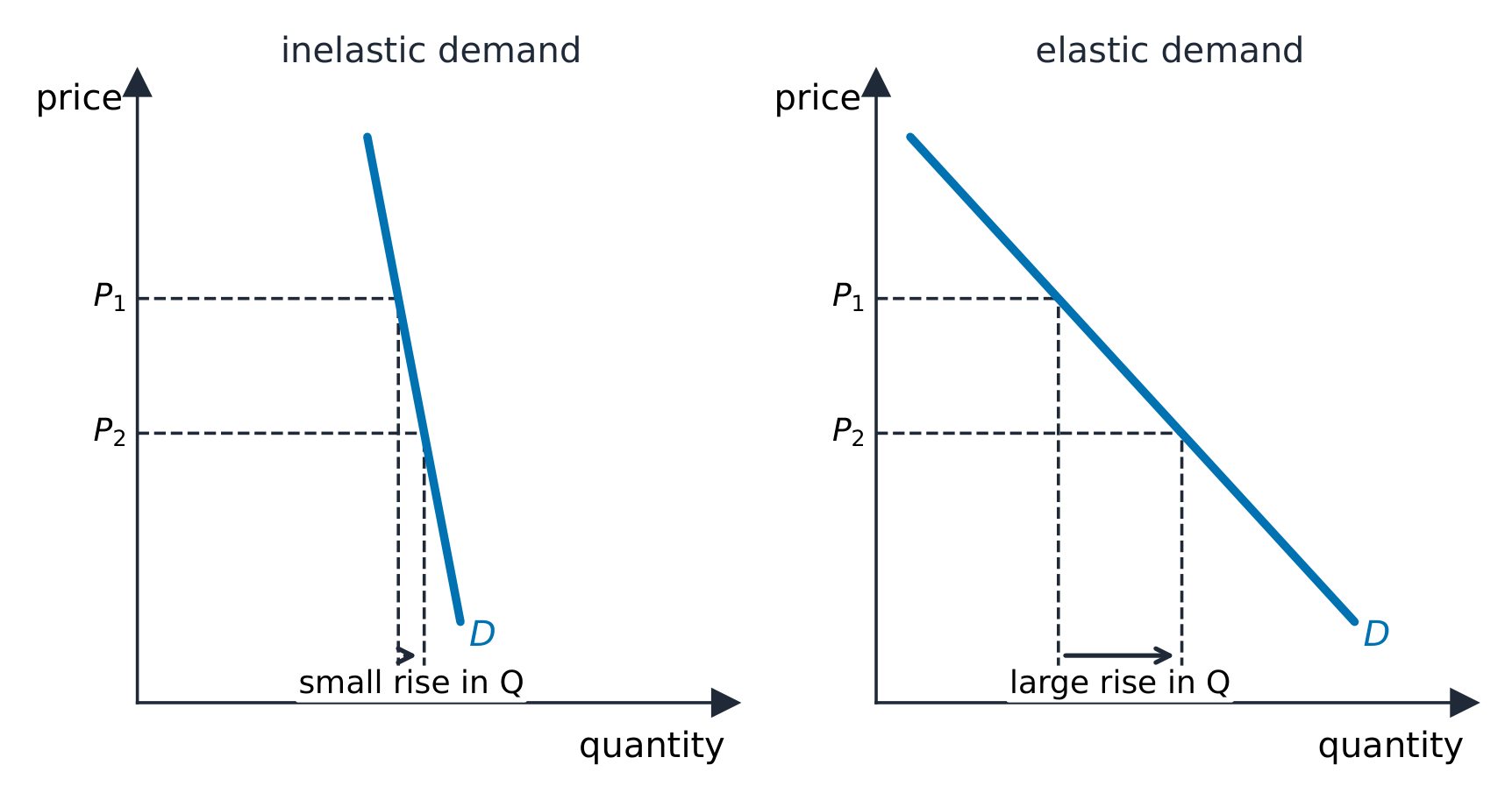
    Price elasticity of demand 需求价格弹性 measures how responsive quantity demanded is to a price change:

    $$E_d=\left|\frac{\%\ \Delta\ \text{quantity demanded}}{\%\ \Delta\ \text{price}}\right|.$$

    • $E_d>1$: elastic 富有弹性 (quantity responds strongly);
    • $E_d<1$: inelastic 缺乏弹性 (quantity barely responds);
    • $E_d=1$: unit elastic.

    Demand is more elastic when there are more substitutes, the good is a luxury, it takes a large share of income, or buyers have more time to adjust. Elasticity links to total revenue 总收入 ($P\times Q$): if demand is elastic, a price cut raises revenue; if inelastic, a price cut lowers it. Along a straight-line demand curve, elasticity falls as you move down (elastic on top, inelastic at the bottom).

    Worked example. A price rise from $\$10$ to $\$12$ (a $+20\%$ change) cuts quantity demanded from $100$ to $85$ (a $-15\%$ change). Then $E_d=\left|\dfrac{-15\%}{20\%}\right|=0.75<1$, so demand is inelastic. Because it is inelastic, the price rise raises total revenue: from $\$10\times100=\$1000$ to $\$12\times85=\$1020$.

    한국어
    수요의 가격 탄력성

    수요의 가격 탄력성은 수요량이 가격 변화에 얼마나 민감하게 반응하는지를 측정한다:

    $$E_d=\left|\frac{\%\ \Delta\ \text{quantity demanded}}{\%\ \Delta\ \text{price}}\right|.$$

    비탄력적 수요와 탄력적 수요: 가격 변화에 대한 작은 반응 vs 큰 반응
    비탄력적 수요와 탄력적 수요: 가격 변화에 따른 작은 반응과 큰 반응
    • $E_d>1$: 탄력적 (수량이 강하게 반응);
    • $E_d<1$: 비탄력적 (수량이 거의 반응하지 않음);
    • $E_d=1$: 단위 탄력적.

    대체재가 많거나, 재화가 사치재이거나, 소득 중 차지하는 비중이 크거나, 구매자가进行调整에 더 많은 시간을 가질 때 수요는 더 탄력적이다. 탄력성은 총수입(Total Revenue) ($P\times Q$)과 연결된다: 수요가 탄력적이면 가격 인하가 수익을 증가시키고, 비탄력적이면 가격 인하가 수익을 감소시킨다. 직선 수요곡선 위에서 아래로 이동할수록 탄력성이 떨어진다(위쪽은 탄력적, 아래쪽은 비탄력적).

    해설 예제. 가격이 $\$10$ to $\$12$로 상승함($+20\%$ 변화)으로 인해 수량 요구가 $100$에서 $85$로 감소함($-15\%$ 변화). 따라서 $E_d=\left|\dfrac{-15\%}{20\%}\right|=0.75<1$이므로, 수요는 비탄력적입니다. 비탄력적이므로 가격 상승은 총수입을 높입니다: $\$10\times100=\$1000$에서 시작하여 $\$12\times85=\$1020$로 증가합니다.

    Explore · ⁨탐색하기⁩

    Stretch price and measure elasticity · ⁨가격을 늘리고 탄력성 측정하기⁩

    Price elasticity of demand is how strongly quantity responds to price. A steep curve is inelastic (small response); a shallow one is elastic (large response). · ⁨수요의 가격 탄력성은 수량이 가격에 얼마나 민감하게 반응하는지를 나타냅니다. 가파른 곡선은 비탄력적(작은 반응), 완만한 곡선은 탄력적(큰 반응)입니다.⁩

    Vocabulary · ⁨어휘⁩ Train · ⁨연습하기⁩
    English 한국어
    elastic/ɪˈlæstɪk/ 탄성 충돌
    inelastic/ɪnɪˈlæstɪk/ 비 탄력적일 때
    total revenue/ˈtəʊtl ˈrevənjuː/ 총매출
    Price elasticity of supply/praɪs ɪlæˈstɪsɪti ɒv səˈplaɪ/ 공급의 가격 탄력성
    Cross-price elasticity/krɒs praɪs ɪlæˈstɪsɪti/ 교체 가격 탄력성
    Income elasticity/ˈɪŋkʌm ɪlæˈstɪsɪti/ 소득 탄력성
    2.4

    Price Elasticity of Supply · ⁨공급의 가격 탄력성⁩

    Syllabus
    English

    Enduring Understanding (MKT-3): Individuals and firms respond to incentives and face constraints.

    Learning Objective MKT-3.E: a. Define measures of elasticity. b. Explain (using graphs where appropriate) measures of elasticity and the impact of a given price change on total revenue or total expenditure. c. Calculate (using data from a graph or a table as appropriate) measures of elasticity.

    • MKT-3.E.6 Price elasticity of supply is measured by the percentage change in quantity supplied divided by the percentage change in price, or the responsiveness of the quantity supplied to changes in price.
    • MKT-3.E.7 Ranges of values of elasticity of supply are described as elastic or inelastic with the separating benchmark being a magnitude of 1, where the change in the price and the change in the quantity supplied are proportional.
      • a. When the magnitude of the value of elasticity is greater than 1, the supply is described as being elastic with respect to that price in the range of the given change.
      • b. When the magnitude of the value of elasticity is less than 1, the supply is described as being inelastic with respect to that price in the range of the given change.
      • c. When the magnitude of the value of elasticity is equal to 1, the supply is described as being unit elastic with respect to that price in the range of the given change.
    • MKT-3.E.8 The price elasticity of supply depends on certain factors such as the price of alternative inputs.
    한국어

    지속적 이해 (MKT-3): 개인과 기업은 유인에 반응하며 제약을 받는다.

    학습 목표 MKT-3.E: a. 탄력성의 측정 지표를 정의하시오. b. 탄력성의 측정 지표와 특정 가격 변화가 총수입 또는 총지출에 미치는 영향을 설명하시오(필요시 그래프 활용). c. 탄력성의 측정 지표를 계산하시오(필요시 그래프나 표의 데이터 활용).

    • MKT-3.E.6 공급의 가격 탄력성은 공급량의 백분율 변화량을 가격의 백분율 변화량으로 나눈 값으로 측정되거나, 공급량이 가격 변화에 얼마나 민감하게 반응하는지로 정의된다.
    • MKT-3.E.7 공급의 탄력성 값 범위는 탄력적(elastic) 또는 비탄력적(inelastic)으로 묘사되며, 이때 구분 기준은 1이라는 크기이며, 이 경우 가격 변화와 공급량 변화가 비례한다.
      • a. 탄력성 값의 크기가 1보다 클 때, 해당 가격에 대해 주어진 변화 범위 내에서 공급은 탄력적이라고 묘사된다.
      • b. 탄력성 값의 크기가 1보다 작을 때, 해당 가격에 대해 주어진 변화 범위 내에서 공급은 비탄력적이라고 묘사된다.
      • c. 탄력성 값의 크기가 1과 같을 때, 해당 가격에 대해 주어진 변화 범위 내에서 공급은 단위 탄력적(unit elastic)이라고 묘사된다.
    • MKT-3.E.8 공급의 가격 탄력성은 교대 투입재의 가격과 같은 특정 요인에 의존한다.

    Source: College Board AP Course and Exam Description · ⁨출처: College Board AP Course and Exam Description⁩

    English

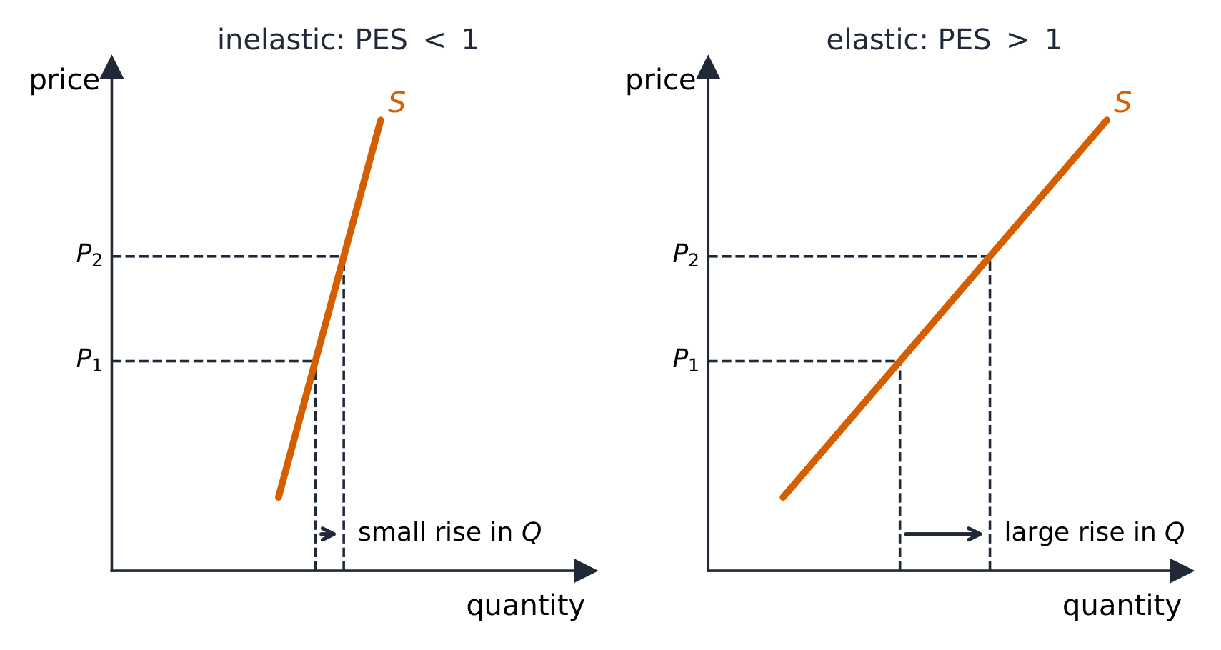
    Price elasticity of supply 供给价格弹性, $E_s=\dfrac{\%\ \Delta\ Q_s}{\%\ \Delta\ P}$, measures how responsive sellers are. Supply is more elastic when firms can adjust output easily – spare capacity, storable goods, and above all more time (supply is more elastic in the long run than the short run).

    한국어

    공급의 가격 탄력성, $E_s=\dfrac{\%\ \Delta\ Q_s}{\%\ \Delta\ P}$,는 판매자가 얼마나 민감하게 반응하는지를 측정한다. 기업이 산출량을 쉽게 조정할 수 있을 때 공급은 더 탄력적이다—여유 용량, 보관 가능한 재화, 그리고 무엇보다 더 많은 시간(장기가 단기에 비해 공급 탄력성이 더 큼).

    PES가 1 미만일 때는 동일한 가격 상승이 작은 공급 반응을, 1 이상일 때는 큰 공급 반응을 나타냄
    PES가 1 미만일 때는 같은 가격 상승이 작은 공급 반응을, 1보다 클 때는 큰 공급 반응을 보인다
    2.5

    Other Elasticities · ⁨기타 탄력성⁩

    Syllabus
    English

    Enduring Understanding (MKT-3): Individuals and firms respond to incentives and face constraints.

    Learning Objective MKT-3.E: a. Define measures of elasticity. b. Explain (using graphs where appropriate) measures of elasticity and the impact of a given price change on total revenue or total expenditure. c. Calculate (using data from a graph or a table as appropriate) measures of elasticity.

    • MKT-3.E.9 Elasticity can be measured for any determinant of demand or supply, not just the price.
    • MKT-3.E.10 Income elasticity of demand is measured by the percentage change in the quantity demanded divided by the percentage change in consumers' income. Economists use the income elasticity of demand to determine whether a good is normal or inferior.
    • MKT-3.E.11 Cross-price elasticity of demand is measured by the percentage change in the quantity demanded of one good divided by the percentage change in the price of another good. Economists use the cross-price elasticity of demand to determine whether goods are substitutes, complements, or not related.
    한국어

    지속적 이해 (MKT-3): 개인과 기업은 유인에 반응하며 제약을 받는다.

    학습 목표 MKT-3.E: a. 탄력성의 측정 지표를 정의하시오. b. 탄력성의 측정 지표와 특정 가격 변화가 총수입 또는 총지출에 미치는 영향을 설명하시오(필요시 그래프 활용). c. 탄력성의 측정 지표를 계산하시오(필요시 그래프나 표의 데이터 활용).

    • MKT-3.E.9 탄력성은 가격뿐만 아니라 수요나 공급을 결정하는 모든 요인에 대해 측정할 수 있다.
    • MKT-3.E.10 수요의 소득 탄력성은 수량의 백분율 변화량을 소비자의 소득의 백분율 변화량으로 나눈 값으로 측정된다. 경제학자는 수요의 소득 탄력성을 사용하여 재화가 정상재(normal good)인지 열등재(inferior good)인지를 판단하는 데 사용한다.
    • MKT-3.E.11 교차 수요 탄력성은 한 재화의 수량 요구량 변화율을 다른 재화의 가격 변화율로 나눈 값으로 측정된다. 경제학자들은 교차 수요 탄력성을 사용하여 재화가 대체재인지, 보완재인지, 아니면 무관한지 판단하는 데 사용한다.

    Source: College Board AP Course and Exam Description · ⁨출처: College Board AP Course and Exam Description⁩

    English
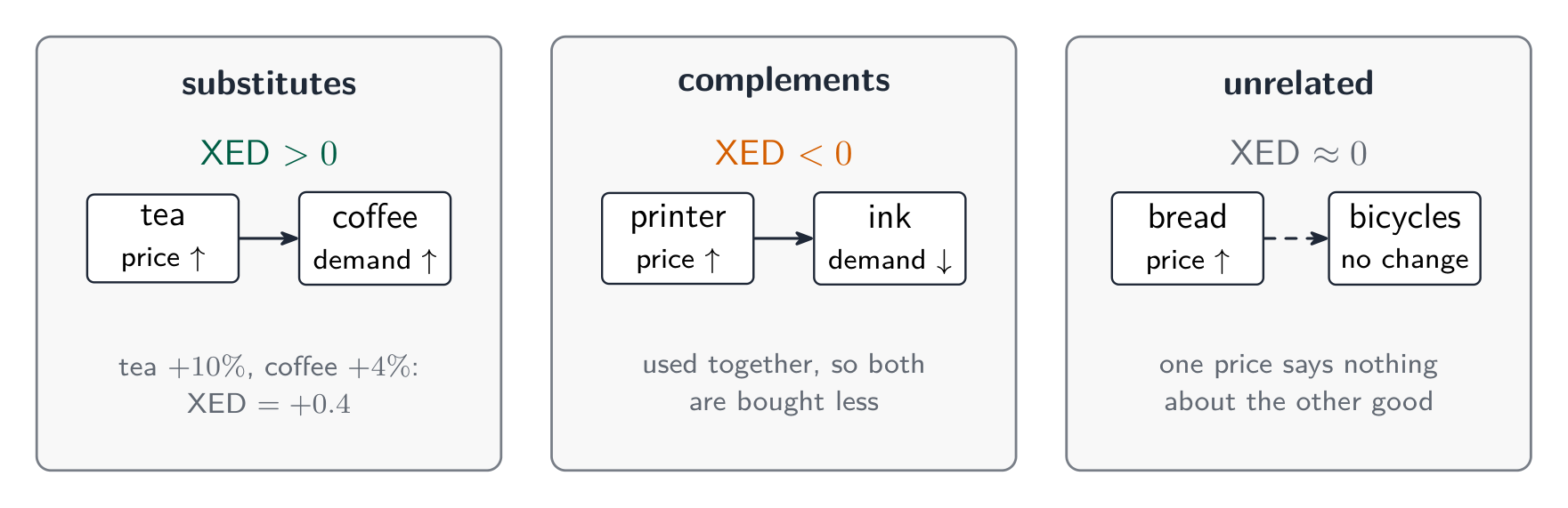
    • Cross-price elasticity 交叉价格弹性 $=\dfrac{\%\ \Delta\ Q_x}{\%\ \Delta\ P_y}$: positive for substitutes, negative for complements – the sign tells you the relationship.
    • Income elasticity 收入弹性 $=\dfrac{\%\ \Delta\ Q}{\%\ \Delta\ \text{income}}$: positive for normal goods (and $>1$ for luxuries), negative for inferior goods.

    Worked example. When the price of coffee rises $10\%$, the quantity of tea demanded rises $6\%$: cross-price elasticity $=\dfrac{+6\%}{+10\%}=+0.6$. The positive sign confirms coffee and tea are substitutes. If instead a $5\%$ rise in incomes raised restaurant-meal demand $10\%$, income elasticity $=\dfrac{10\%}{5\%}=+2$ – a normal good, and a luxury since it exceeds $1$.

    Exam skill: you are expected to compute an elasticity, classify it, and read a sign as evidence of substitute/complement or normal/inferior.

    한국어
    • 교차가격 탄력성 $=\dfrac{\%\ \Delta\ Q_x}{\%\ \Delta\ P_y}$: 대체재에서는 양수, 보완재에서는 음수—부호는 관계를 나타낸다.
    • 소득 탄력성 $=\dfrac{\%\ \Delta\ Q}{\%\ \Delta\ \text{income}}$: 정상재(그리고 사치재인 경우 $>1$ 이상)에서는 양수, 저급재에서는 음수.

    해설 예시. 커피의 가격이 $10\%$ 상승하면, 차에 대한 수요량이 $6\%$ 증가한다: 교차가격 탄력성 $=\dfrac{+6\%}{+10\%}=+0.6$. 양(+) 의 부호는 커피와 차가 대체재임을 확인시켜 준다. 만약 소득이 $5\%$ 상승하여 레스토랑 식사 수요가 $10\%$ 증가했다면, 이는 소득 탄력성 $=\dfrac{10\%}{5\%}=+2$ – 정품이며, $1$를 초과하므로 고급재이다.

    교차탄력성: 대체재는 양(-), 보완재는 음(-)
    교차탄력성: 대체재는 양(-), 보완재는 음(-)

    시험 기술: 탄력성을 계산하고, 이를 분류하며, 부호를 대체재/보완재 또는 정품/저급품의 증거로 읽어야 한다.

    2.6

    Market Equilibrium, Consumer Surplus, and Producer Surplus · ⁨시장 균형, 소비자余유, 생산자余유⁩

    Syllabus
    English

    Enduring Understanding (MKT-4): Although equilibria are stable, an economy can move from one equilibrium to another if market conditions change.

    Learning Objective MKT-4.A: a. Define (using graphs as appropriate) market equilibrium, consumer surplus, and producer surplus. b. Explain (using graphs as appropriate) how equilibrium price, quantity, consumer surplus, and producer surplus for a good or service are determined. c. Calculate (using data from a graph or table as appropriate) areas of consumer surplus and producer surplus at equilibrium.

    • MKT-4.A.1 The supply-demand model is a tool for understanding what factors influence prices and quantities and why prices and quantities might differ across markets or change over time.
    • MKT-4.A.2 In a perfectly competitive market, equilibrium is achieved (and markets clear with no shortages or surpluses) when the price of a good or service brings the quantity supplied and quantity demanded into balance, in the sense that buyers wish to purchase the same quantity that sellers wish to provide.
    • MKT-4.A.3 Equilibrium price provides information to economic decision-makers to guide resource allocation.
    • MKT-4.A.4 Economists use consumer surplus and producer surplus to measure the benefits markets create to buyers and sellers and understand market efficiency.
    • MKT-4.A.5 Market equilibrium maximizes total economic surplus in the absence of market failures, meaning that perfectly competitive markets are efficient.
    한국어

    지속적 이해 (MKT-4): 균형은 안정적이지만 시장 조건이 변하면 경제가 한 균형에서 다른 균형으로 이동할 수 있다.

    학습 목표 MKT-4.A: a. 시장 균형, 소비자 ErrorMessage, 생산자 ErrorMessage를 정의하시오(적절할 경우 그래프 사용). b. 특정 재화나 서비스의 균형 가격, 수량, 소비자 ErrorMessage, 생산자 ErrorMessage가 어떻게 결정되는지 설명하시오(적절할 경우 그래프 사용). c. 적절할 경우 그래프나 표의 데이터를 사용하여 균형 시의 소비자 ErrorMessage와 생산자 ErrorMessage 면적을 계산하시오.

    • MKT-4.A.1 수요-공급 모델은 어떤 요인이 가격과 수량에 영향을 미치는지, 그리고 왜 가격과 수량이 시장 간 또는 시간에 따라 달라질 수 있는지를 이해하기 위한 도구이다.
    • MKT-4.A.2 완벽 경쟁 시장에서 균형(수급이 일치하여 공백이나 과잉 없이 시장이 청산됨)은 재화나 서비스의 가격이 공급 수량과 수요 수량을 조화시키는 수준일 때 달성되며, 이는 구매자가 원하는 수량이 판매자가 제공하려는 수량과 동일함을 의미한다.
    • MKT-4.A.3 균형 가격은 경제적 의사결정자에게 자원 배분에 대한 정보를 제공하여 가이드 역할을 한다.
    • MKT-4.A.4 경제학자들은 소비자와 생산자가create하는 이익을 측정하고 시장의 효율성을 이해하기 위해 소비자 ErrorMessage와 생산자 ErrorMessage를 사용한다.
    • MKT-4.A.5 시장 실패가 없는 상황에서 시장 균형은 총 경제적 ErrorMessage를 극대화하므로, 완벽 경쟁 시장은 효율적이다.

    Source: College Board AP Course and Exam Description · ⁨출처: College Board AP Course and Exam Description⁩

    English
    Consumer & producer surplus

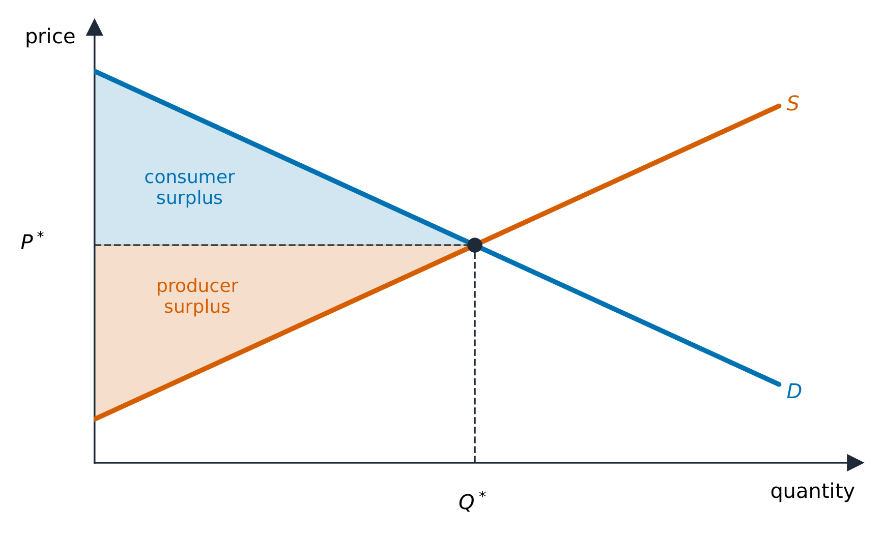
    Equilibrium 均衡 is where supply meets demand: the equilibrium price clears the market, so quantity demanded equals quantity supplied and there is no shortage or surplus.

    • Consumer surplus 消费者剩余 is the area below the demand curve and above the price – the gap between what buyers would pay and what they do pay.
    • Producer surplus 生产者剩余 is the area above the supply curve and below the price – the gap between the price and sellers' minimum acceptable price.
    • Their sum is total surplus 总剩余, and the competitive equilibrium maximizes it – this is why free markets are called allocatively efficient 配置有效率.
    한국어
    소비자 & 생산자 surplus

    균형은 공급과 수요가 만나는 지점이다: 균형 가격은 시장을 청산하여, 수요량과 공급량이 같아지고 과잉수요나 과잉공급이 없다.

    시장 균형 상태에서의 소비자가잉여와 생산자가잉여
    시장 균형 상태에서의 소비자가잉여와 생산자가잉여
    • 소비자余유는 수요 곡선 아래이고 가격 위에 있는 영역 – 구매자가 지불할 금액과 실제 지불하는 금액 사이의 차이이다.
    • 생산자余유는 공급 곡선 위이고 가격 아래에 있는 영역 – 가격과 판매자의 최소 허용 가격 사이의 차이이다.
    • 두 값의 합은 총余유이며, 경쟁적 균형은 이를 최대화한다 – 이것이 자유 시장이 배분 효율적이라고 불리는 이유이다.
    과일과 야채를 파는 시장 가판대
    실제 시장: 많은 구매자와 판매자가 만나, 원하는 수량이 제공된 수량과 같아지는 지점에서 가격이 결정됨
    Explore · ⁨탐색하기⁩

    See consumer and producer surplus · ⁨소비자 surplus(초과)와 생산자 surplus(초과) 보기⁩

    At equilibrium the market clears. The gap between what buyers would pay and the price is consumer surplus; the gap above sellers' costs is producer surplus. · ⁨균형에서 시장은 청산됩니다. 구매자가 지불하려 했던 금액과 실제 가격 사이의 차이가 **소비자 surplus(초과)**이며, 판매자의 비용보다 높은 차이는 **생산자 surplus(초과)**입니다.⁩

    Vocabulary · ⁨어휘⁩ Train · ⁨연습하기⁩
    English 한국어
    Producer surplus/prəˈdjuːsə ˈsɜːpləs/ 생산자 잔여
    total surplus/ˈtəʊtl ˈsɜːpləs/ 총잉여
    allocatively efficient/ˈæləkətɪvli ɪˈfɪʃənt/ 배당 효율적
    surplus/ˈsɜːpləs/ 초과를 초래한다
    shortage/ˈʃɔːtɪdʒ/ 부족을 초래한다
    2.7

    Market Disequilibrium and Changes in Equilibrium · ⁨시장 비균형 및 균형 변화⁩

    Syllabus
    English

    Enduring Understanding (MKT-4): Although equilibria are stable, an economy can move from one equilibrium to another if market conditions change.

    Learning Objective MKT-4.B: a. Define a surplus and shortage. b. Explain (using graphs where appropriate) how changes in underlying conditions and shocks to a competitive market can alter price, quantity, consumer surplus, and producer surplus. c. Calculate (using data from a graph or table as appropriate) changes in price, quantity, consumer surplus, and producer surplus in response to changes in market conditions or market disequilibrium.

    • MKT-4.B.1 Whenever markets experience imbalances—creating disequilibrium prices and quantities, surpluses, and shortages—market forces drive price and quantity toward equilibrium.
    • MKT-4.B.2 Factors that shift the market demand and market supply curves cause price, quantity, consumer surplus, producer surplus, and total economic surplus (within that market) to change. The impact of the change depends on the price elasticities of demand and supply.
    한국어

    지속적 이해 (MKT-4): 균형은 안정적이지만 시장 조건이 변하면 경제가 한 균형에서 다른 균형으로 이동할 수 있다.

    학습 목표 MKT-4.B: a. 과잉과 부족을 정의하십시오. b. 적절할 경우 그래프를 사용하여 경쟁 시장에 대한 하위 조건 변화와 충격이 가격, 수량, 소비자 ErrorMessage, 생산자 ErrorMessage에 어떻게 영향을 미치는지 설명하시오. c. 적절할 경우 그래프나 표의 데이터를 사용하여 시장 조건 변화 또는 시장 비균형에 따른 가격, 수량, 소비자 ErrorMessage, 생산자 ErrorMessage의 변화를 계산하시오.

    • MKT-4.B.1 시장이 불균형을 겪어 비균형 가격과 수량, 과잉, 부족을 초래할 때마다 시장 힘은 가격과 수량을 균형 방향으로 유도한다.
    • MKT-4.B.2 시장 수요 곡선과 시장 공급 곡선을 이동시키는 요인은 가격, 수량, 소비자 ErrorMessage, 생산자 ErrorMessage, 그리고 해당 시장의 총 경제적 ErrorMessage를 변화시킨다. 이 변화의 영향은 수요와 공급의 가격 탄력성에 따라 다르다.

    Source: College Board AP Course and Exam Description · ⁨출처: College Board AP Course and Exam Description⁩

    English

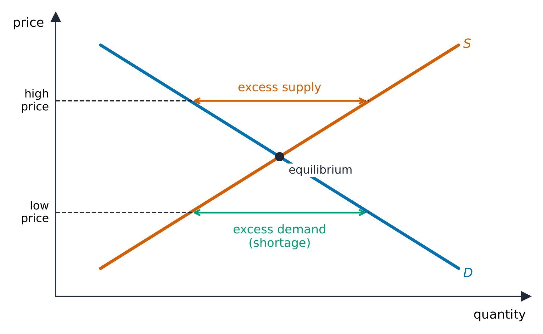
    Away from equilibrium the market self-corrects: above the equilibrium price there is a surplus 过剩 (excess supply) that pushes price down; below it a shortage 短缺 (excess demand) that pushes price up.

    When a determinant shifts a curve, the equilibrium moves predictably. A single shift gives a definite result for both price and quantity. When both curves shift, one of price or quantity is indeterminate (depends on the relative sizes of the shifts) – a favorite exam trap. Work these out by drawing the shifts.

    한국어

    균형에서 벗어난 시장에서는 자체적으로 교정된다: 균형 가격 위에는 과잉공급이 있어 가격을 낮추고, 아래에는 과잉수요가 있어 가격을 높인다.

    균형 위에는 과잉공급; 아래에는 과잉수요
    균형 위에는 과잉공급; 아래에는 과잉수요

    결정 요인이 곡선을 이동시키면 균형이 예측 가능하게 움직인다. 단일 이동은 가격과 수량 모두에 명확한 결과를 가져온다. 양쪽 곡선이 모두 이동할 때, 가격이나 수량 중 하나는 불확정적이다(이동의 상대적 크기에 따름) – 시험의的经典陷阱。이것들은 이동을 그려서 풀어야 한다.

    Vocabulary · ⁨어휘⁩ Train · ⁨연습하기⁩
    English 한국어
    Equilibrium/ˌiːkwɪˈlɪbrɪəm/ 평형
    Consumer surplus/kənˈsuːmə ˈsɜːpləs/ 소비자 잔여
    2.8

    The Effects of Government Intervention in Markets · ⁨정부의 시장 개입 효과⁩

    Syllabus
    English

    Enduring Understanding (POL-1): Government policies influence consumer and producer behavior and therefore affect market outcomes.

    Learning Objective POL-1.A: a. Define forms of government price and quantity intervention. b. Explain (using graphs where appropriate) how government policies alter consumer and producer behaviors that influence incentives and therefore affect outcomes. c. Calculate (using data from a graph or table where appropriate) changes in market outcomes resulting from government policies.

    • POL-1.A.1 Some government policies, such as price floors, price ceilings, and other forms of price and quantity regulation, affect incentives and outcomes in all market structures.
    • POL-1.A.2 Governments use taxes and subsidies to change incentives in ways that influence consumer and producer behavior, shifting the supply and demand curves accordingly.
    • POL-1.A.3 Taxes and subsidies affect government revenues or costs.
    • POL-1.A.4 Government intervention in a market producing the efficient quantity through taxes, subsidies, price controls, or quantity controls can only decrease allocative efficiency.
    • POL-1.A.5 Deadweight loss represents the losses to buyers and sellers as a result of government intervention in an efficient market.
    • POL-1.A.6 The incidence of taxes and subsidies imposed on goods traded in perfectly competitive markets depends on the elasticity of supply and demand.
    한국어

    지속적 이해 (POL-1): 정부 정책은 소비자와 생산자의 행동에 영향을 미치므로 시장 결과에도 영향을 준다.

    학습 목표 POL-1.A: a. 정부의 가격 및 수량 개입 형태를 정의하시오. b. 적절할 경우 그래프를 사용하여 정부 정책이 인센티브에 영향을 미침으로써 소비자와 생산자의 행동을 어떻게 변경시키고 이로 인해 결과가 달라지는지 설명하시오. c. 적절할 경우 그래프나 표의 데이터를 사용하여 정부 정책에 따른 시장 결과의 변화를 계산하시오.

    • POL-1.A.1 최저가, 최고가 등 가격 및 수량 규제 등의 일부 정부 정책은 모든 시장 구조에서 인센티브와 결과에 영향을 미친다.
    • POL-1.A.2 정부는 세금과 보조금을 사용하여 소비자와 생산자의 행동에 영향을 미치는 방식으로 인센티브를 변화시키며, 이에 따라 공급 및 수요 곡선이 이동한다.
    • POL-1.A.3 세금과 보조금은 정부의 세수 또는 비용에 영향을 미친다.
    • POL-1.A.4 세금, 보조금, 가격 통제 또는 수량 통제를 통해 효율적인 수량을 생산하는 시장에 대한 정부 개입은 배분 효율성만 감소시킬 수 있다.
    • POL-1.A.5 사각지대 손실(Deadweight loss)은 효율적인 시장에서 정부 개입으로 인한 구매자와 판매자의 손실을 나타낸다.
    • POL-1.A.6 완벽 경쟁 시장에서 거래되는 재화에 부과된 세금과 보조금의 부담(세입부담)은 공급과 수요의 탄력성에 의존한다.

    Source: College Board AP Course and Exam Description · ⁨출처: College Board AP Course and Exam Description⁩

    English
    A price ceiling causes a shortage
    A tax and the deadweight loss

    Governments intervene, usually reducing total surplus:

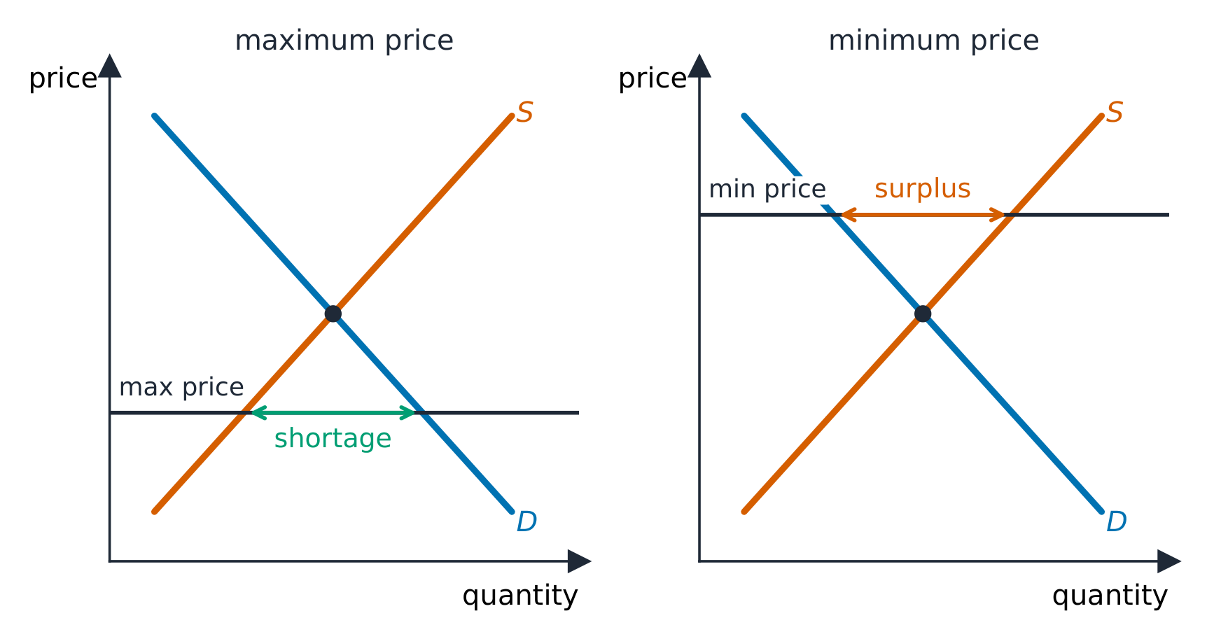
    • A price ceiling 价格上限 (a legal maximum, like rent control) below equilibrium causes a persistent shortage.
    • A price floor 价格下限 (a legal minimum, like a minimum wage) above equilibrium causes a persistent surplus.
    • An excise tax 消费税 shifts supply up by the tax; the burden (tax incidence 税收归宿) falls more heavily on whichever side is more inelastic.
    • A subsidy shifts supply down, raising quantity.

    Each of these creates deadweight loss 无谓损失 – mutually beneficial trades that no longer happen, shown as a triangle between the curves at the new quantity.

    Exam skill: on a graph, be able to shade consumer surplus, producer surplus, government revenue from a tax, and deadweight loss, and say who bears the tax and why.

    한국어
    가격 상한선이 과잉수요를 유발함
    세금과 무효 손실

    정부는 보통 총余유를 감소시키는 방식으로 개입한다:

    가격 상한선은 부족을, 가격 하한선은 과잉 공급을 유발함
    가격 상한선이 과잉수요를 유발하고, 가격 하한선이 과잉공급을 유발함
    • 가격 상한선 (임대료 규제와 같은 법적 최대액)이 균형보다 낮으면persistent한 과잉수요가 발생한다.
    • 가격 하한선 (최저임금과 같은 법적 최소액)이 균형보다 높으면persistent한 과잉공급이 발생한다.
    • 소모세는 세금만큼 공급 곡선을 위로 이동시키고, 부담(세목 전가)은 더 불탄력적인 쪽에 더 크게fall한다.
    • 보조금은 공급 곡선을 아래로 이동시켜 수량을 늘린다.

    이들 모두는 무효 손실을 발생시킨다 – 새로운 수량에서 곡선 사이에서 삼각형으로 표시되는 더 이상 일어나지 않는 상호 유익적인 거래들이다.

    시험 기술: 그래프 위에서 소비자余유, 생산자余유, 세금으로부터의 정부 세수, 그리고 무효 손실을 채우며, 누가 세금을 부담하고 그 이유를 설명할 수 있어야 한다.

    Explore · ⁨탐색하기⁩

    Add a tax or price control · ⁨세금이나 가격 통제 추가하기⁩

    A price ceiling below equilibrium causes shortages; a tax drives a wedge between what buyers pay and sellers get, shrinking the quantity traded. · ⁨가격 상한선이 균형보다 낮으면 부족 현상이 발생하며, 세금은 구매자가支付的金额과 판매자가 받는 금액 사이에 격차를 만들어 거래 수량을 축소시킵니다.⁩

    Vocabulary · ⁨어휘⁩ Train · ⁨연습하기⁩
    English 한국어
    price ceiling/praɪs ˈsiːlɪŋ/ 가격 상한선
    price floor/praɪs flɔː/ 가격 하한선
    excise tax/ekˈsaɪz tæks/ 소모세
    tax incidence/tæks ˈɪnsɪdəns/ 세 부담
    deadweight loss/ˈdedweɪt lɒs/ 无谓损失
    world price/wɜːld praɪs/ 세계 가격
    imports/ɪmˈpɔːts/ 수입의 증대를 의미한다.
    exports/ˈekspɔːts/ 수출
    2.9

    International Trade and Public Policy · ⁨국제 무역 및 공공 정책⁩

    Syllabus
    English

    Enduring Understanding (POL-1): Government policies influence consumer and producer behavior and therefore affect market outcomes.

    Learning Objective POL-1.B: a. Define tariffs and quotas. b. Explain (using graphs where appropriate) how markets are affected by public policy related to international trade. c. Calculate (using data from a graph or table as appropriate) changes in market outcomes resulting from public policy related to international trade.

    • POL-1.B.1 Equilibria in competitive markets may be altered by the decision to open an economy to trade with other countries; equilibrium price can be higher or lower than under autarky, and the gap between domestic supply and demand is filled by trade. Opening an economy to trade with other countries affects consumer surplus, producer surplus, and total economic surplus.
    • POL-1.B.2 Tariffs, which governments sometimes use to influence international trade, affect domestic price, quantity, government revenue, and consumer surplus and total economic surplus.
    • POL-1.B.3 Quotas can be used to alter quantities produced and therefore affect price, consumer surplus, and total economic surplus.
      • Exclusion statement: The graphing of quotas is beyond the scope of the course and the AP Exam, but understanding how quotas affect quantities produced is within the scope.
    한국어

    지속적 이해 (POL-1): 정부 정책은 소비자와 생산자의 행동에 영향을 미치므로 시장 결과에도 영향을 준다.

    학습 목표 POL-1.B: a. 관세와 수입 제한_quota_을 정의하시오. b. 적절할 경우 그래프를 사용하여 국제 무역 관련 공공 정책이 시장에 미치는 영향을 설명하시오. c. 적절할 경우 그래프나 표의 데이터를 사용하여 국제 무역 관련 공공 정책에 따른 시장 결과의 변화를 계산하시오.

    • POL-1.B.1 경쟁 시장의 균형은 국가间 무역을 위한 경제 개방 결정에 의해 변경될 수 있으며, 균형 가격은 자족 상태下的보다 높거나 낮을 수 있고, 국내 공급과 수요의 격차는 무역을 통해 메워진다. 경제를 타국과의 무역에 개방하면 소비자 ErrorMessage, 생산자 ErrorMessage, 총 경제적 ErrorMessage에 영향을 미친다.
    • POL-1.B.2 정부가 국제 무역에 영향을 주기 위해时使用하는 관세는 국내 가격, 수량, 정부 세수, 소비자 ErrorMessage 및 총 경제적 ErrorMessage에 영향을 미친다.
    • POL-1.B.3 수입 제한_quota_은 생산 수량을 변경하기 위해 사용될 수 있으므로 가격, 소비자 ErrorMessage, 총 경제적 ErrorMessage에 영향을 미친다.
      • 제외 사항: 수입 quota_의 그래프 작성은 과정 및 AP 시험 범위를 벗어나지만, 수입 quota_이 생산 수량에 미치는 영향을 이해하는 것은 범위 내에 포함된다.

    Source: College Board AP Course and Exam Description · ⁨출처: College Board AP Course and Exam Description⁩

    English

    When a country opens to trade at a world price 世界价格:

    • If the world price is below the domestic price, the country imports 进口 – consumers gain more than producers lose, so total surplus rises.
    • If the world price is above the domestic price, the country exports 出口 – producers gain more than consumers lose.

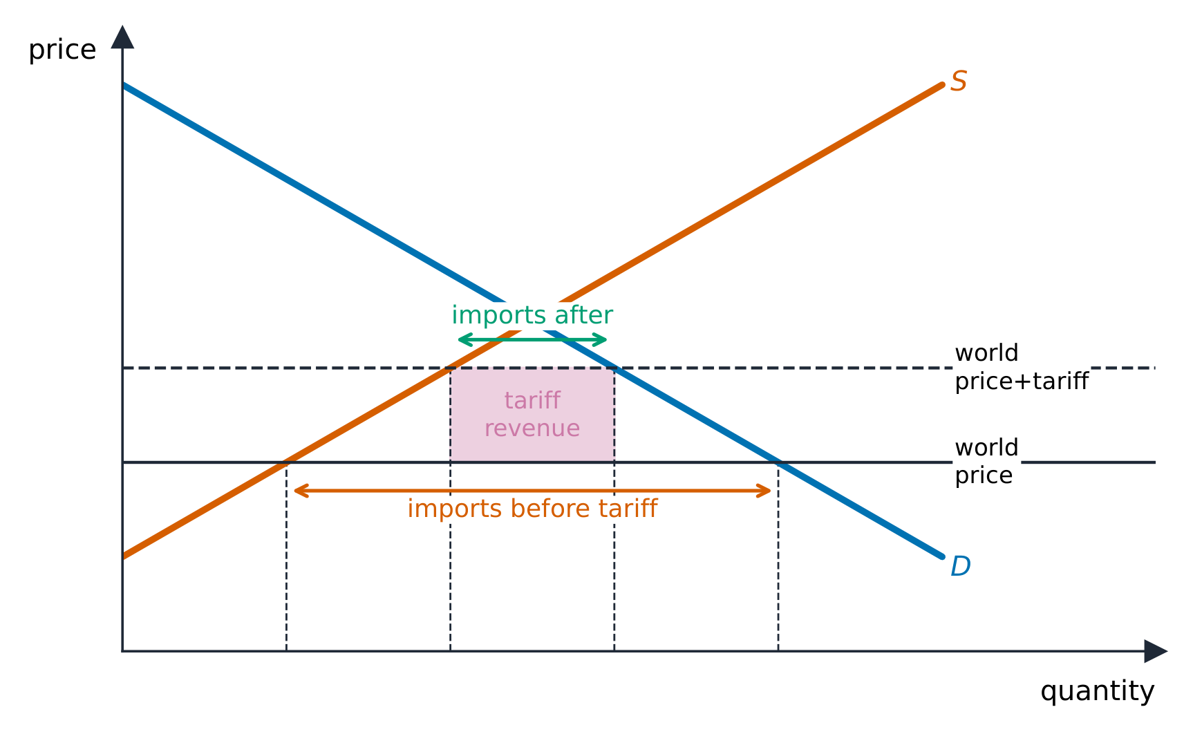
    A tariff 关税 (a tax on imports) or a quota 配额 (a limit on imports) raises the domestic price, helps domestic producers, hurts consumers more, and creates deadweight loss. Free trade maximizes total surplus, which is the core efficiency argument for it.

    한국어

    한 국가가 세계 가격으로 무역을 열 때:

    관세는 국내 공급을 늘리고 수요를 줄이며 수입을 축소함
    관세는 국내 공급을 늘리고 수요를 줄이며 수입을 축소함
    • 세계 가격이 국내 가격보다 낮으면,该国是수입국 – 소비자의 이득이 생산자의 손실보다 커서 총余유가 증가한다.
    • 세계 가격이 국내 가격보다 높으면,该国是수출국 – 생산자의 이득이 소비자의 손실보다 크다.

    관세(수입에 부과되는 세금) 또는 수입 quota(수입 제한)는 국내 가격을 높여 국내 생산자를 돕고 소비자에게 더 큰 피해를 주며 무효 손실을 만든다. 자유 무역은 총余유를 극대화하므로 이것이 자유 무역의 핵심 효율성 논리이다.

    Vocabulary · ⁨어휘⁩ Train · ⁨연습하기⁩
    English 한국어
    tariff/ˈtærɪf/ 관세
    quota/ˈkwəʊtə/ 수입 quota
    2.9

    Exam tips · ⁨시험 팁⁩

    English
    • Separate a movement along a curve (own price) from a shift (a determinant); a single shift gives a definite result, a double shift leaves one variable indeterminate.
    • Compute elasticity $E_d=|\%\Delta Q \div \%\Delta P|$; elastic ($>1$) means a price cut raises total revenue, inelastic ($<1$) lowers it.
    • Read the sign of cross-price elasticity (substitutes $+$, complements $-$) and income elasticity (normal $+$, inferior $-$).
    • Shade consumer/producer surplus and the deadweight loss from a tax or price control; incidence falls on the more inelastic side.
    • A price ceiling below equilibrium causes a shortage; a price floor above causes a surplus.
    한국어
    • 곡선 위의 이동(자신 가격)과 이동(결정 요인)을 구분하라; 단일 이동은 명확한 결과를 내지만, 이중 이동은 하나의 변수를 불확정적으로 만든다.
    • 탄력성을 계산한다 $E_d=|\%\Delta Q \div \%\Delta P|$; 탄력적($>1$)이면 가격 인하가 총수입을 늘리고, 비탄력적($<1$)이면 줄인다.
    • 교차가격 탄력성의 부호를 읽는다(대체재 $+$, 보완재 $-$)와 소득 탄력성을 읽는다(정품 $+$, 저급품 $-$).
    • 세금이나 가격 통제로부터의 소비자/생산자余유와 무효 손실을 채우고, 부담이 더 불탄력적인 쪽에fall함을 명시한다.
    • 균형 이하의 가격 상한선은 과잉수요를, 균형 이상의 가격 하한선은 과잉공급을 유발한다.
  • 3

    Production, Cost, and the Perfect Competition Model · ⁨생산, 비용 및 완전 경쟁 모델⁩

    Watch lesson · ⁨수업 보기⁩
    3.1

    The Production Function

    Syllabus
    English

    Enduring Understanding (PRD-1): Firms' production and cost constraints over different input and output levels shape optimal decisions in the short run and long run.

    Learning Objective PRD-1.A: a. Define (using graphs where appropriate) key terms and concepts relating to production and cost. b. Explain (using graphs where appropriate) how production and cost are related in the short run and long run. c. Calculate (using data from a graph or table as appropriate) the various measures of productivity and short-run and long-run costs.

    • PRD-1.A.1 The production function explains the relationship between inputs and outputs both in the short run and the long run.
    • PRD-1.A.2 Marginal product and average product change as input usage changes, and hence, total product changes.
    • PRD-1.A.3 Diminishing marginal returns occur as the firm employs more of one input, holding other inputs constant, to produce a product (output) in the short run.
    한국어

    지속적 이해 (PRD-1): 기업의 생산 및 비용 제약 조건이 입력 및 출력 수준에 따라 단기 및 장기에서 최적의 의사결정을 형성한다.

    학습 목표 PRD-1.A: a. (그림이 필요한 경우 그림을 사용하여) 생산 및 비용과 관련된 주요 용어 및 개념을 정의하시오. b. (그림이 필요한 경우 그림을 사용하여) 단기 및 장기에서 생산과 비용이 어떻게 관련되는지 설명하시오. c. (그래프나 표의 데이터를 사용하는 경우가 필요한 경우) 다양한 생산성 지표와 단기 및 장기 비용을 계산하시오.

    • PRD-1.A.1 생산 함수는 단기 및 장期的에 inputs와 outputs 사이의 관계를 설명한다.
    • PRD-1.A.2 입력 사용량이 변화함에 따라 한계생산량과 평균생산량이 변하므로 총생산량도 변한다.
    • PRD-1.A.3 단기에 기업이 하나의 입력만을 증가시키고 다른 입력들은 일정하게 유지하여 제품(출력)을 생산할 때 한계수익체감현상이 발생한다.

    Source: College Board AP Course and Exam Description · ⁨출처: College Board AP Course and Exam Description⁩

    A steel plant: production functions and costs shape how firms supply goods
    A steel plant: production functions and costs shape how firms supply goods

    The production function 生产函数 links inputs to output. In the short run 短期 at least one input (usually capital) is fixed 固定; in the long run 长期 all inputs vary.

    • Total product 总产量 is the total output.
    • Marginal product 边际产量 (MP) is the extra output from one more unit of a variable input (usually labor): $MP=\dfrac{\Delta\ \text{output}}{\Delta\ \text{labor}}$.
    • Average product 平均产量 is output per worker.

    As you add workers to fixed capital, MP eventually falls – the law of diminishing marginal returns 边际收益递减法则. This shape of MP is what drives the shape of the cost curves below.

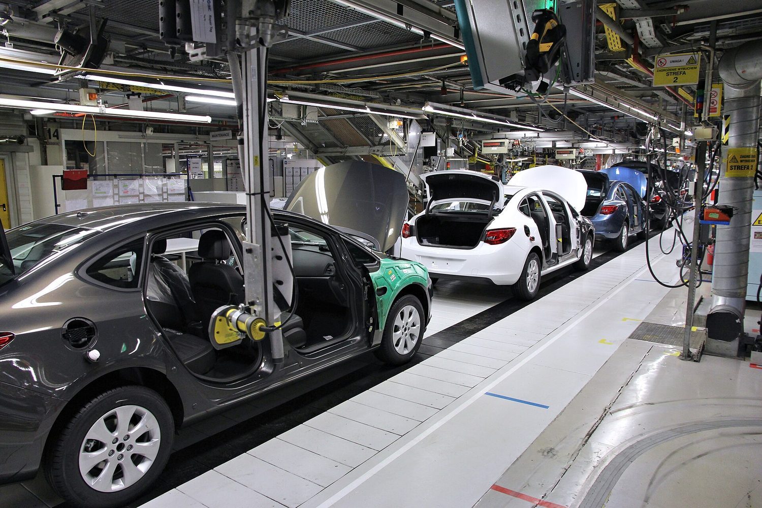
    A robotic arm working on a factory production line
    The production function turns inputs — labour and capital like this robot — into output
    Vocabulary · ⁨어휘⁩ Train · ⁨연습하기⁩
    English 한국어
    production function/prəˈdʌkʃn ˈfʌŋkʃn/ 생산 함수
    short run/ʃɔːt rʌn/ 단기
    fixed/fɪkst/ 고정된다
    long run/lɒŋ rʌn/ 장기
    Total product/ˈtəʊtl ˈprɒdʌkt/ 총생산
    Marginal product/ˈmɑːdʒɪnl ˈprɒdʌkt/ 한계생산
    Average product/ˈævrɪdʒ ˈprɒdʌkt/ 평균생산
    law of diminishing marginal returns/lɔː ɒv dɪˈmɪnɪʃɪŋ ˈmɑːdʒɪnl rɪˈtɜːnz/ 한계 수익 체감의 법칙
    3.2

    Short-Run Production Costs

    Syllabus
    English

    Enduring Understanding (PRD-1): Firms' production and cost constraints over different input and output levels shape optimal decisions in the short run and long run.

    Learning Objective PRD-1.A: a. Define (using graphs where appropriate) key terms and concepts relating to production and cost. b. Explain (using graphs where appropriate) how production and cost are related in the short run and long run. c. Calculate (using data from a graph or table as appropriate) the various measures of productivity and short-run and long-run costs.

    • PRD-1.A.4 Fixed costs and variable costs determine the total cost.
    • PRD-1.A.5 Marginal cost, average (fixed, variable, and total) cost, total cost, and total variable cost change as total output changes, but total fixed cost remains constant at all output levels, including zero output.
    • PRD-1.A.6 Production functions with diminishing marginal returns yield an upward-sloping marginal cost curve.
    • PRD-1.A.7 Specialization and the division of labor reduce marginal costs for firms.
    • PRD-1.A.8 Cost curves can shift in response to changes in input costs and productivity.
    한국어

    지속적 이해 (PRD-1): 기업의 생산 및 비용 제약 조건이 입력 및 출력 수준에 따라 단기 및 장기에서 최적의 의사결정을 형성한다.

    학습 목표 PRD-1.A: a. (그림이 필요한 경우 그림을 사용하여) 생산 및 비용과 관련된 주요 용어 및 개념을 정의하시오. b. (그림이 필요한 경우 그림을 사용하여) 단기 및 장기에서 생산과 비용이 어떻게 관련되는지 설명하시오. c. (그래프나 표의 데이터를 사용하는 경우가 필요한 경우) 다양한 생산성 지표와 단기 및 장기 비용을 계산하시오.

    • PRD-1.A.4 고정비와 변동비는 총비용을 결정한다.
    • PRD-1.A.5 총생산량이 변화함에 따라 한계비용, 평균(고정, 변동, 총)비용, 총비용 및 총변동비가 변하지만, 총고정비는 모든 출력 수준(0 출력 포함)에서 일정하다.
    • PRD-1.A.6 한계수익체감현상을 나타내는 생산 함수는 우상향하는 한계비용 곡선을 산출한다.
    • PRD-1.A.7 전문성과 노동의 분업은 기업의 한계비용을 낮춘다.
    • PRD-1.A.8 입력 비용 및 생산성의 변화에 따라 비용 곡선이 이동할 수 있다.

    Source: College Board AP Course and Exam Description · ⁨출처: College Board AP Course and Exam Description⁩

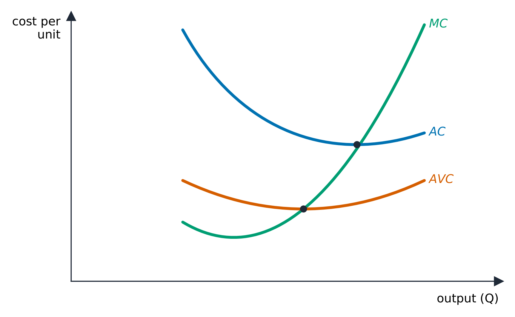
    Short-run cost curves (MC, ATC, AVC)

    Costs split into fixed and variable:

    The short-run marginal, average, and average variable cost curves
    The short-run marginal, average, and average variable cost curves
    • Fixed cost 固定成本 (FC) does not change with output (rent on the factory).
    • Variable cost 可变成本 (VC) rises with output (materials, labor).
    • Total cost 总成本 $TC=FC+VC$.

    The per-unit costs matter most:

    • Average fixed cost $AFC=FC/Q$ falls continuously (spreading fixed cost).
    • Average variable cost $AVC=VC/Q$ and average total cost $ATC=TC/Q$ are U-shaped.
    • Marginal cost 边际成本 $MC=\dfrac{\Delta TC}{\Delta Q}$ is the cost of one more unit.

    Two key facts: MC is the mirror image of MP (when MP rises, MC falls, and vice versa), and MC cuts both AVC and ATC at their minimum points (when marginal is below average, the average falls; when above, it rises).

    Worked example. A firm has fixed cost $FC=\$100$. At $Q=10$ its total cost is $\$300$, so variable cost is $\$200$: then $ATC=\tfrac{300}{10}=\$30$, $AVC=\tfrac{200}{10}=\$20$, and $AFC=\tfrac{100}{10}=\$10$ (note $AFC+AVC=ATC$). If raising output to $Q=11$ pushes total cost to $\$325$, the marginal cost of that $11$th unit is $\dfrac{\Delta TC}{\Delta Q}=\dfrac{325-300}{1}=\$25$.

    Explore · ⁨탐색하기⁩

    Explore the U-shaped cost curves · ⁨U자형 비용 곡선 탐구하기⁩

    As output rises, marginal cost eventually climbs (diminishing returns) and cuts through the U-shaped average cost at its minimum — the most efficient scale. · ⁨생산량이 증가함에 따라 한계비용이 eventually 상승(한계报酬 감소)하여 U자형 평균비용의 최소점을 지나갑니다—가장 효율적인 규모입니다.⁩

    Vocabulary · ⁨어휘⁩ Train · ⁨연습하기⁩
    English 한국어
    Fixed cost/fɪkst kɒst/ 고정비
    Variable cost/ˈveərɪəbl kɒst/ 변동비
    Total cost/ˈtəʊtl kɒst/ 총 비용
    Marginal cost/ˈmɑːdʒɪnl kɒst/ AC가 최소인 지점
    3.3

    Long-Run Production Costs

    Syllabus
    English

    Enduring Understanding (PRD-1): Firms' production and cost constraints over different input and output levels shape optimal decisions in the short run and long run.

    Learning Objective PRD-1.A: a. Define (using graphs where appropriate) key terms and concepts relating to production and cost. b. Explain (using graphs where appropriate) how production and cost are related in the short run and long run. c. Calculate (using data from a graph or table as appropriate) the various measures of productivity and short-run and long-run costs.

    • PRD-1.A.9 In the long run, firms can adjust all their inputs, and as a result, all costs become variable.
    • PRD-1.A.10 The relationship between inputs and outputs in the long run is described by the scale of production—increasing, decreasing, or constant returns to scale.
    • PRD-1.A.11 The long-run average total cost is characterized by economies of scale, diseconomies of scale, or constant returns to scale (efficient scale).
    • PRD-1.A.12 The minimum efficient scale plays a role in determining the concentration of firms in a market and the market structure.
    한국어

    지속적 이해 (PRD-1): 기업의 생산 및 비용 제약 조건이 입력 및 출력 수준에 따라 단기 및 장기에서 최적의 의사결정을 형성한다.

    학습 목표 PRD-1.A: a. (그림이 필요한 경우 그림을 사용하여) 생산 및 비용과 관련된 주요 용어 및 개념을 정의하시오. b. (그림이 필요한 경우 그림을 사용하여) 단기 및 장기에서 생산과 비용이 어떻게 관련되는지 설명하시오. c. (그래프나 표의 데이터를 사용하는 경우가 필요한 경우) 다양한 생산성 지표와 단기 및 장기 비용을 계산하시오.

    • PRD-1.A.9 장기에는 기업이 모든 입력을 조정할 수 있으므로 결과적으로 모든 비용이 변동비가 된다.
    • PRD-1.A.10 장기에서의 입력과 출력 간의 관계는 규모에 따른 수익성—증가, 감소 또는 일정—로 설명된다.
    • PRD-1.A.11 장기평균총비용은 규모의 경제, 규모의 비경제 또는 일정规模에 따른 수익성(효율적 규모)으로 특징지어진다.
    • PRD-1.A.12 최소 효율적 규모는 시장의 기업 밀집도를 결정하고 시장 구조에 영향을 미친다.

    Source: College Board AP Course and Exam Description · ⁨출처: College Board AP Course and Exam Description⁩

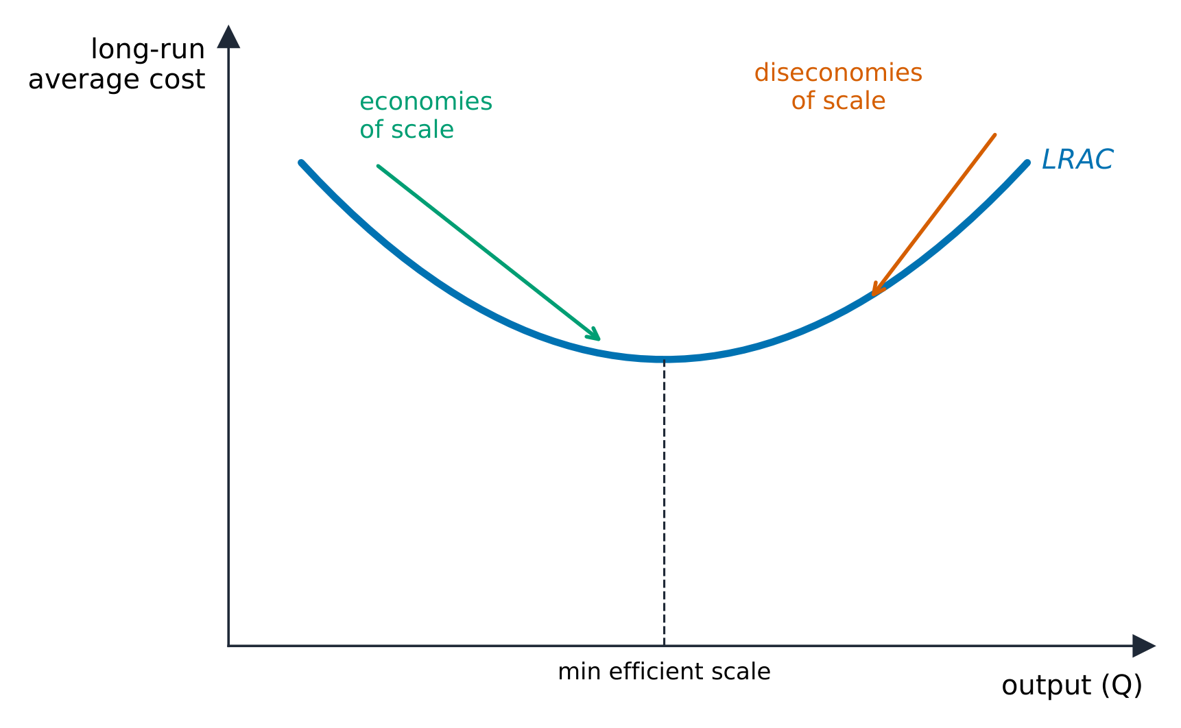
    In the long run all inputs – including plant size – can change, so only the long-run average total cost (LRATC) curve matters. Its shape shows returns to scale:

    Economies and diseconomies of scale on the long-run average cost curve
    Economies and diseconomies of scale on the long-run average cost curve
    • Economies of scale 规模经济: LRATC falls as output grows (bulk buying, specialization).
    • Constant returns to scale: LRATC flat.
    • Diseconomies of scale 规模不经济: LRATC rises (a firm too big to manage well).

    Exam skill: know that "diminishing returns" is a short-run idea (one fixed input) while "economies of scale" is a long-run idea (all inputs vary) – examiners test the distinction.

    Vocabulary · ⁨어휘⁩ Train · ⁨연습하기⁩
    English 한국어
    Economies of scale/ɪˈkɒnəmiz ɒv skeɪl/ 규모의 경제
    Diseconomies of scale/ˌdɪsɪˈkɒnəmiz ɒv skeɪl/ Diseconomies of scale
    3.4

    Types of Profit

    Syllabus
    English

    Enduring Understanding (CBA-2): To determine the optimal level at which to pursue an activity whose total benefits exceed total cost, rational economic agents compare marginal benefits and marginal costs.

    Learning Objective CBA-2.C: a. Define the different types of profit. b. Explain how firms respond to profit opportunities. c. Calculate a firm's profit or loss.

    • CBA-2.C.1 Firms respond to economic profit (loss) rather than accounting profit.
    • CBA-2.C.2 Accounting profit fails to account for implicit costs (such as cost of financial capital, compensation for risk, or an entrepreneur's time), which, if fully compensated, result in normal profit.
    한국어

    지속적 이해 (CBA-2): 총 편익이 총 비용 초과일 때 어떤 활동을 추구할 최적 수준을 결정하기 위해 합리적 경제 주체는 한계 편익과 한계 비용을 비교한다.

    학습 목표 CBA-2.C: a. 다양한 유형의 이익을 정의하시오. b. 기업이 이익 기회에 어떻게 대응하는지 설명하시오. c. 기업의 이익 또는 손실을 계산하시오.

    • CBA-2.C.1 기업은 회계이익이 아닌 경제이익(손실)에 대응한다.
    • CBA-2.C.2 회계이익은 암묵적 비용(금융 자본의 비용, 위험에 대한 보상, 사업가의 시간 등)을 고려하지 못하는데, 이를 완전히 보전하면 정상이익이 발생한다.

    Source: College Board AP Course and Exam Description · ⁨출처: College Board AP Course and Exam Description⁩

    Economists count all opportunity costs, including the owner's:

    • Explicit costs 显性成本 are out-of-pocket payments; implicit costs 隐性成本 are the opportunity costs of owner-supplied resources (forgone salary, forgone interest).
    • Accounting profit 会计利润 $=$ revenue $-$ explicit costs.
    • Economic profit 经济利润 $=$ revenue $-$ explicit $-$ implicit costs.

    Because economic profit subtracts more, it is smaller. Zero economic profit (a normal profit 正常利润) still means the owner is earning exactly the opportunity cost of their resources – a perfectly acceptable outcome.

    Worked example. A shopkeeper takes in $\$200{,}000$ of revenue and pays $\$120{,}000$ in explicit costs, so accounting profit is $\$80{,}000$. But she gave up a $\$70{,}000$ salary elsewhere and $\$5{,}000$ of interest on the savings she invested – $\$75{,}000$ of implicit costs. Her economic profit is $80{,}000-75{,}000=\$5{,}000$: still positive, so staying in business genuinely beats her next-best alternative.

    Vocabulary · ⁨어휘⁩ Train · ⁨연습하기⁩
    English 한국어
    Explicit costs/ekˈsplɪsɪt kɒsts/ 명시 비용
    implicit costs/ɪmˈplɪsɪt kɒsts/ 명시되지 않은 비용
    Accounting profit/əˈkaʊntɪŋ ˈprɒfɪt/ 회계 이익
    Economic profit/ˌiːkəˈnɒmɪk ˈprɒfɪt/ 경제 이익
    normal profit/ˈnɔːml ˈprɒfɪt/ 정상 이득
    3.5

    Profit Maximization

    Syllabus
    English

    Enduring Understanding (CBA-2): To determine the optimal level at which to pursue an activity whose total benefits exceed total cost, rational economic agents compare marginal benefits and marginal costs.

    Learning Objective CBA-2.D: a. Define (using graphs or data as appropriate) the profit-maximizing rule. b. Explain (using a graph or data as appropriate) the profit-maximizing level of production.

    • CBA-2.D.1 Firms are assumed to produce output to maximize their profits by comparing marginal revenue and marginal cost.
    한국어

    지속적 이해 (CBA-2): 총 편익이 총 비용 초과일 때 어떤 활동을 추구할 최적 수준을 결정하기 위해 합리적 경제 주체는 한계 편익과 한계 비용을 비교한다.

    학습 목표 CBA-2.D: a. (그림이나 데이터가 필요한 경우) 이윤 극대화 규칙을 정의하시오. b. (그림이나 데이터가 필요한 경우) 이윤 극대화를 위한 생산 수준을 설명하시오.

    • CBA-2.D.1 기업은 한계수입과 한계비용을 비교하여 이윤을 극대화하는 출력을 생산한다고 가정한다.

    Source: College Board AP Course and Exam Description · ⁨출처: College Board AP Course and Exam Description⁩

    Every firm, in every market structure, maximizes profit at the quantity where marginal revenue equals marginal cost:

    $$MR=MC.$$
    Produce each unit whose MR exceeds its MC; stop when they are equal. Producing less leaves profitable units unmade; producing more adds units that cost more than they earn.

    3.6

    Deciding to Produce, Enter, or Exit

    Syllabus
    English

    Enduring Understanding (PRD-2): Firms' short-run decisions to produce output, and long-run decisions to enter or exit a market, are based on profitability.

    Learning Objective PRD-2.A: Explain (using graphs or data where appropriate) firms' short-run decisions to produce positive output levels, or long-run decisions to enter or exit a market in response to profit-making opportunities.

    • PRD-2.A.1 In the short run, firms decide to operate (i.e., produce positive output) or shut down (i.e., produce zero output) by comparing total revenue to total variable cost or price to average variable cost (AVC).
    • PRD-2.A.2 In the absence of barriers to entry or exit, in the long run (i.e., once factors that are fixed in the short run become variable), firms enter a market in which there are profit-making opportunities and exit a market when they anticipate economic losses.
    한국어

    지속적 이해 (PRD-2): 기업의 단기 생산 의사결정과 시장의 진입·퇴출 장기 의사결정은 수익성에 기반한다.

    학습 목표 PRD-2.A: (그림이나 데이터가 필요한 경우) 기업이 이익 창출 기회에 responding하여 양의 출력 수준을 생산하거나 시장에 진입·퇴출하는 단기 및 장기 의사결정을 설명하시오.

    • PRD-2.A.1 단기에서 기업은 총수익을 총변동비와 비교하거나 가격을 평균변동비(AVC)와 비교하여 운영(즉, 양의 출력 생산)하거나停产(즉, 0 출력 생산) 여부를 결정한다.
    • PRD-2.A.2 진입·퇴출 장벽이 없는 경우, 장기에서(즉, 단기에 고정된 요인이 변동이 된 후) 기업은 이익 기회가 있는 시장에 진입하고 경제적 손실이 예상될 때는 퇴출한다.

    Source: College Board AP Course and Exam Description · ⁨출처: College Board AP Course and Exam Description⁩

    Even at $MR=MC$, a firm must check whether to operate:

    • Short run – the shutdown rule: keep producing only if price covers average variable cost ($P\geq AVC$). If $P, shut down and lose only fixed cost. So the firm's short-run supply curve is its MC curve above minimum AVC.
    • Profit check: compare $P$ to $ATC$ at the profit-maximizing quantity – $P>ATC$ means economic profit, $P means a loss, $P=ATC$ means break-even.
    • Long run – entry and exit: economic profits attract entry 进入; losses cause exit 退出. This continues until economic profit is zero.
    Vocabulary · ⁨어휘⁩ Train · ⁨연습하기⁩
    English 한국어
    entry/ˈentri/ 진입
    exit/ˈeɡzɪt/ 퇴출
    3.7

    Perfect Competition

    Syllabus
    English

    Enduring Understanding (PRD-3): Even with a common goal of profit-maximization, market structure constrains and influences prices, output, and efficiency.

    Learning Objective PRD-3.A: a. Define (using graphs as appropriate) the characteristics of perfectly competitive markets and efficiency. b. Explain (using graphs where appropriate) equilibrium and firm decision making in perfectly competitive markets and how prices in perfectly competitive markets lead to efficient outcomes. c. Calculate (using data from a graph or table as appropriate) economic profit (loss) in perfectly competitive markets.

    • PRD-3.A.1 A perfectly competitive market is efficient. Firms in perfectly competitive markets face no barriers to entry and have no market power.
    • PRD-3.A.2 In perfectly competitive markets, prices communicate to consumers and producers the magnitude of others' marginal costs of production and marginal benefits of consumption and provide incentives to act on that information (i.e., price equals marginal cost in an efficient market).
    • PRD-3.A.3 In perfectly competitive markets, firms can sell all their outputs at a constant price determined by the market.
    • PRD-3.A.4 At a competitive market equilibrium, firms are price takers and select output to maximize profit by producing the level of output where the marginal cost equals marginal revenue (at the price).
    • PRD-3.A.5 At a competitive market equilibrium, the price of a product equals both the private marginal benefit received by the last unit consumed and the private marginal cost incurred to produce the last unit, thus achieving allocative efficiency.
    • PRD-3.A.6 In a short-run competitive equilibrium, price can either be above or below its long-run competitive level resulting in profits or losses, motivating entry or exit of firms and moving prices and quantities toward long-run equilibrium.
    • PRD-3.A.7 In a long-run perfectly competitive equilibrium, productive efficiency implies all operating firms produce at efficient scale, price equals marginal cost and minimum average total cost, and firms earn zero economic profit.
    • PRD-3.A.8 Firms may be in a constant cost, increasing cost, or decreasing cost industry. Long-run prices depend on the portion of the long-run cost curves on which firms operate.
    • PRD-3.A.9 A perfectly competitive market in long-run equilibrium is allocatively and productively efficient.
    한국어

    지속적 이해 (PRD-3): 이윤 극대화를 위한 공통된 목표를 가지더라도 시장 구조는 가격, 출력 및 효율성을 제한하고 영향을 미친다.

    학습 목표 PRD-3.A: a. (그림이 필요한 경우) 완전경쟁 시장의 특성과 효율성을 정의하시오. b. (그림이 필요한 경우) 완전경쟁 시장의 균형과 기업의 의사결정을 설명하고, 완전경쟁 시장의 가격이 어떻게 효율적인 결과를 초래하는지 설명하시오. c. (그래프나 표의 데이터를 사용하는 경우가 필요한 경우) 완전경쟁 시장의 경제이익(손실)을 계산하시오.

    • PRD-3.A.1 완전경쟁 시장은 효율적이다. 완전경쟁 시장의 기업은 진입 장벽이 없고 시장 지배력이 없다.
    • PRD-3.A.2 완전경쟁 시장에서 가격은 소비자와 생산자에게 타인의 한계생산비용 및 한계소비편익의 크기를 전달하며, 그 정보를 바탕으로 행동할 동기를 제공한다(즉, 효율적 시장에서는 가격이 한계비용과 같다).
    • PRD-3.A.3 완전경쟁 시장에서 기업은 시장이 결정하는 일정한 가격으로 모든 출력을 판매할 수 있다.
    • PRD-3.A.4 경쟁 시장 균형에서 기업은 가격 수용자이며, 한계비용이 한계수익과 같아지는 출력 수준을 생산함으로써(가격에서) 이윤을 극대화하는 출력을 선택한다.
    • PRD-3.A.5 경쟁 시장 균형에서 상품의 가격은 마지막 단위가 소비됨에 따라 얻는 사적 한계 편익과 마지막 단위를 생산하는 데 드는 사적 한계 비용과 같아지므로 배분 효율성이 달성됩니다.
    • PRD-3.A.6 단기 경쟁 균형에서는 가격이 장기 경쟁 수준보다 높거나 낮을 수 있어 이득이나 손실을 초래하며, 이는 기업의 진입이나 퇴출을 촉진하고 가격 및 수량을 장기 균형으로 이동시킵니다.
    • PRD-3.A.7 장기 완전경쟁 균형에서 생산 효율성은 모든 운영 기업이 효율적 규모로 생산함을 의미하며, 가격은 한계 비용과 최소 평균 총비용과 같고 기업은 영(零)의 경제적 이득을 얻습니다.
    • PRD-3.A.8 기업은 일정 비용, 증가 비용 또는 감소 비용 산업에 속할 수 있습니다. 장기 가격은 기업이 운영하는 장기 비용 곡선의 부분에 따라 결정됩니다.
    • PRD-3.A.9 장기 균형 상태인 완전경쟁 시장은 배분 효율적이고 생산 효율적입니다.

    Source: College Board AP Course and Exam Description · ⁨출처: College Board AP Course and Exam Description⁩

    A perfectly competitive 完全竞争 market has many small firms, an identical (homogeneous) product, free entry and exit, and perfect information. Each firm is a price taker 价格接受者 – too small to affect the price – so it faces a horizontal demand curve at the market price, and price = marginal revenue = average revenue ($P=MR=AR$).

    This is why economists prize perfect competition. In long-run equilibrium it is both allocatively efficient 配置效率 and productively efficient 生产效率. Allocative efficiency holds because the firm produces where $P = MC$: the price (society's marginal benefit from the last unit) equals its marginal cost, so exactly the right amount is made. Productive efficiency holds because free entry drives price down to the minimum of average total cost, so goods are made as cheaply as possible. The market price is itself a signal that communicates everyone's marginal costs and benefits.

    The market sets the price; the price-taking firm produces where MC = P, here with short-run profit
    The market sets the price; the price-taking firm produces where MC = P, here with short-run profit

    The side-by-side panel is the graph the exam wants: the market (left) fixes the price $P^{*}$; the firm (right) takes it as a horizontal line and produces where $MC=P$. When $P>ATC$ there is a short-run profit (the shaded box); that profit attracts entry, which shifts market supply right and pushes the price down.

    A perfectly competitive firm makes only normal profit in the long run
    A perfectly competitive firm makes only normal profit in the long run
    • Short run: the firm can earn profit, break even, or take a loss, producing where $P=MC$.
    • Long run: entry and exit drive the firm to zero economic profit, producing where $P=MC=ATC$ at minimum ATC. This double efficiency – productive efficiency (lowest-cost output) and allocative efficiency ($P=MC$, so the last unit's value equals its cost) – is the benchmark against which every other market structure is judged.

    Exam skill: be able to draw the side-by-side market and single-firm graphs, show a short-run profit or loss, then show how entry/exit restores long-run equilibrium at minimum ATC.

    Explore · ⁨탐색하기⁩

    A price-taking firm in a competitive market · ⁨경쟁 시장에서의 가격 수용 기업⁩

    In perfect competition the market sets the price and each firm is a price-taker. It produces where price equals marginal cost, earning zero economic profit in the long run. · ⁨완전 경쟁에서 시장이 가격을 설정하고 각 기업은 가격 수용자입니다. 기업은 가격이 한계비용과 같아지는 지점에서 생산하며, 장기적으로 0의 경제적 이익을 얻습니다.⁩

    Vocabulary · ⁨어휘⁩ Train · ⁨연습하기⁩
    English 한국어
    perfectly competitive/ˈpɜːfektlɪ kəmˈpetɪtɪv/ 완전 경쟁
    price taker/praɪs ˈteɪkə/ 가격 수용자
    allocatively efficient/ˈæləkətɪvli ɪˈfɪʃənt/ 배당 효율적
    productively efficient/prəˈdʌktɪvli ɪˈfɪʃənt/ 생산 효율성
    3.7

    Exam tips

    • Know the cost curves: AFC falls, ATC/AVC are U-shaped, and MC cuts ATC and AVC at their minimums.
    • Every firm maximises profit at MR = MC; check the shutdown rule ($P \ge AVC$ in the short run).
    • Distinguish accounting profit (revenue − explicit costs) from economic profit (also minus implicit/opportunity costs); zero economic profit is normal.
    • "Diminishing returns" is short-run (one fixed input); "economies of scale" is long-run (all inputs vary).
    • In perfect competition $P=MR=AR$; entry/exit drive long-run economic profit to zero at minimum ATC.
  • 4

    Imperfect Competition · ⁨불완전 경쟁⁩

    Watch lesson · ⁨수업 보기⁩
    4.1

    Imperfect Competition and Market Power

    Syllabus
    English

    Enduring Understanding (PRD-3): Even with a common goal of profit-maximization, market structure constrains and influences prices, output, and efficiency.

    Learning Objective PRD-3.B: a. Define (using graphs where appropriate) the characteristics of imperfectly competitive markets and inefficiency.

    • PRD-3.B.1 Imperfectly competitive markets include monopoly, oligopoly, and monopolistic competition in product markets and monopsony in factor markets.
    • PRD-3.B.2 In imperfectly competitive output markets and assuming all else is constant, a firm must lower price to sell additional units.
    • PRD-3.B.3 In imperfectly competitive markets, consumers and producers respond to prices that are above the marginal costs of production and/or marginal benefits of consumption (i.e., price is greater than marginal cost in an inefficient market).
    • PRD-3.B.4 Incentives to enter an industry may be mitigated by barriers to entry. Barriers to entry—such as high fixed/start-up costs, legal barriers to entry, and exclusive ownership of key resources—can sustain imperfectly competitive market structures.
    한국어

    지속적 이해 (PRD-3): 이윤 극대화를 위한 공통된 목표를 가지더라도 시장 구조는 가격, 출력 및 효율성을 제한하고 영향을 미친다.

    학습 목표 PRD-3.B: a. (적절한 경우 그래프를 사용하여) 불완전경쟁 시장의 특징과 비효율성을 정의합니다.

    • PRD-3.B.1 불완전경쟁 시장에는 제품 시장의 독점, 과점, 제품 차별화 경쟁과 요인 시장의 독점 매수자가 포함됩니다.
    • PRD-3.B.2 불완전경쟁의 산출 시장에서 기타 조건이 동일하다고 가정할 때, 기업은 추가 단위를 판매하기 위해 가격을 인하해야 합니다.
    • PRD-3.B.3 불완전경쟁 시장에서 소비자와 생산자는 생산 한계 비용 및/또는 소비 한계 편익보다 높은 가격에 대응합니다(즉, 비효율적인 시장에서는 가격이 한계 비용보다 큼).
    • PRD-3.B.4 산업 진입 유인은 진입 장벽에 의해 완화될 수 있습니다. 높은 고정비/초기 투자 비용, 법적 진입 장벽, 핵심 자원의 독점 소유와 같은 진입 장벽은 불완전경쟁 시장 구조를 유지시킬 수 있습니다.

    Source: College Board AP Course and Exam Description · ⁨출처: College Board AP Course and Exam Description⁩

    A car assembly line: market power and firm scale differ under imperfect competition
    A car assembly line: market power and firm scale differ under imperfect competition

    Most real markets are imperfectly competitive 不完全竞争: firms have some market power 市场势力 – the ability to set price rather than take it. The source of that power is a downward-sloping demand curve facing the firm, which means that to sell one more unit the firm must lower the price on all units.

    Market structures range from perfect competition to monopoly
    Market structures range from perfect competition to monopoly

    Because of this, marginal revenue is below price ($MR) for every firm with market power. On a straight-line demand curve the MR curve has the same intercept but twice the slope, lying below demand. This one fact – $MR – separates every imperfect market from perfect competition and explains why they produce less and charge more.

    Worked example. A firm with market power faces demand $P=100-Q$. Selling $1$ unit gives $P=\$99$ and total revenue $\$99$; selling a $2$nd forces the price down to $\$98$ on both units, so revenue rises to $2\times98=\$196$. The marginal revenue of that $2$nd unit is $196-99=\$97$ – below its $\$98$ price. In general $MR=100-2Q$, falling twice as fast as demand.

    Vocabulary · ⁨어휘⁩ Train · ⁨연습하기⁩
    English 한국어
    imperfectly competitive/ɪmˈpɜːfektlɪ kəmˈpetɪtɪv/ 불완전 경쟁
    market power/ˈmɑːkɪt ˈpaʊə/ 시장 지배력
    4.2

    Monopoly

    Syllabus
    English

    Enduring Understanding (PRD-3): Even with a common goal of profit-maximization, market structure constrains and influences prices, output, and efficiency.

    Learning Objective PRD-3.B: b. Explain (using graphs where appropriate) equilibrium, firm decision making, consumer surplus, producer surplus, profit (loss), and deadweight loss in imperfectly competitive markets and why prices in imperfectly competitive markets cannot be relied on to coordinate the actions of all possible market participants and can lead to inefficient outputs. c. Calculate (using data from a graph or table as appropriate) areas of consumer surplus, producer surplus, profit (loss), and deadweight loss in imperfectly competitive markets.

    • PRD-3.B.5 A monopoly exists because of barriers to entry.
    • PRD-3.B.6 In a monopoly, equilibrium (profit-maximizing) quantity is determined by equating marginal revenue (MR) to marginal cost (MC). The price charged is greater than the marginal cost.
      • Equation: $MR = MC$
    • PRD-3.B.7 In a natural monopoly, long-run economies of scale for a single firm exist throughout the entire effective demand of its product.
    한국어

    지속적 이해 (PRD-3): 이윤 극대화를 위한 공통된 목표를 가지더라도 시장 구조는 가격, 출력 및 효율성을 제한하고 영향을 미친다.

    학습 목표 PRD-3.B: b. (적절한 경우 그래프를 사용하여) 불완전경쟁 시장에서의 균형, 기업의 의사결정, 소비자 여력, 생산자 여력, 이득(손실), 그리고 사각지대 손실을 설명하고, 불완전경쟁 시장의 가격이 모든 가능한 시장 참여자의 행동을 조율하는 데 의존할 수 없으며 비효율적인 산출을 초래할 수 있는 이유를 설명합니다. c. (적절한 경우 그래프나 표의 데이터를 사용하여) 불완전경쟁 시장에서의 소비자 여력, 생산자 여력, 이득(손실), 사각지대 손실의 면적을 계산합니다.

    • PRD-3.B.5 독점은 진입 장벽 때문에 존재합니다.
    • PRD-3.B.6 독점에서 균형(이득 극대화) 수량은 한계 수익(MR)을 한계 비용(MC)과 같게 함으로써 결정됩니다. 부과되는 가격은 한계 비용보다 높습니다.
      • 식: $MR = MC$
    • PRD-3.B.7 자연 독점에서 단일 기업의 장기 규모의 경제는其产品의 전체 유효 수요 범위 전반에 걸쳐 존재합니다.

    Source: College Board AP Course and Exam Description · ⁨출처: College Board AP Course and Exam Description⁩

    Monopoly: MR = MC pricing

    A monopoly 垄断 is a single seller of a product with no close substitutes, protected by barriers to entry 进入壁垒 (economies of scale – a natural monopoly 自然垄断 – control of a key resource, patents, or government license).

    A monopoly maximises profit where MC = MR and can earn supernormal profit
    A monopoly maximises profit where MC = MR and can earn supernormal profit
    • The monopolist maximizes profit at $MR=MC$, then charges the highest price the demand curve allows at that quantity (read price up to the demand curve, not the MR curve).
    • Compared with perfect competition it produces less and charges more, earning long-run economic profit because entry is blocked.
    • This under-production creates deadweight loss 无谓损失 – the monopoly is allocatively inefficient because $P>MC$: the last unit is worth more than it costs, yet is not made.

    Governments may respond with antitrust 反垄断 law, or regulate a natural monopoly's price toward $P=MC$ (socially optimal, but may cause a loss) or $P=ATC$ (fair-return, break-even).

    Exam skill: the monopoly graph is a staple – show quantity at $MR=MC$, price up on the demand curve, and shade profit (between $P$ and $ATC$) and deadweight loss (the triangle to the competitive quantity).

    A large utility plant: monopoly and market power mean a single firm can set price above marginal cost
    A large utility plant: monopoly and market power mean a single firm can set price above marginal cost
    Explore · ⁨탐색하기⁩

    A monopoly's cost curves · ⁨독점 기업의 비용 곡선⁩

    A monopoly is the sole seller, so it faces the whole downward demand curve and its marginal revenue lies below price. It produces where MR = MC — less output, higher price than competition. · ⁨독점은 유일한 판매자이므로 전체 하향 수요 곡선에 직면하며, 한계수익은 가격보다 낮습니다. MR = MC인 지점에서 생산하므로, 경쟁보다 적은 산출과 높은 가격을 형성합니다.⁩

    Vocabulary · ⁨어휘⁩ Train · ⁨연습하기⁩
    English 한국어
    monopoly/məˈnɒpəli/ 독점
    barriers to entry/ˈbærɪəz tʊ ˈentri/ 진입 장벽
    natural monopoly/ˈnætʃərəl məˈnɒpəli/ 자연 독점
    deadweight loss/ˈdedweɪt lɒs/ 无谓损失
    antitrust/ˌæntɪˈtrʌst/ 반독점
    4.3

    Price Discrimination

    Syllabus
    English

    Enduring Understanding (PRD-3): Even with a common goal of profit-maximization, market structure constrains and influences prices, output, and efficiency.

    Learning Objective PRD-3.B: b. Explain (using graphs where appropriate) equilibrium, firm decision making, consumer surplus, producer surplus, profit (loss), and deadweight loss in imperfectly competitive markets and why prices in imperfectly competitive markets cannot be relied on to coordinate the actions of all possible market participants and can lead to inefficient outputs. c. Calculate (using data from a graph or table as appropriate) areas of consumer surplus, producer surplus, profit (loss), and deadweight loss in imperfectly competitive markets.

    • PRD-3.B.8 A firm with market power can engage in price discrimination to increase its profits or capture additional consumer surplus under certain conditions.
    • PRD-3.B.9 With perfect price discrimination, a monopolist produces the quantity where price equals marginal cost (just as a competitive market would) but extracts all economic surplus associated with its product and eliminates all deadweight loss.
      • Equation: $P = MC$
    한국어

    지속적 이해 (PRD-3): 이윤 극대화를 위한 공통된 목표를 가지더라도 시장 구조는 가격, 출력 및 효율성을 제한하고 영향을 미친다.

    학습 목표 PRD-3.B: b. (적절한 경우 그래프를 사용하여) 불완전경쟁 시장에서의 균형, 기업의 의사결정, 소비자 여력, 생산자 여력, 이득(손실), 그리고 사각지대 손실을 설명하고, 불완전경쟁 시장의 가격이 모든 가능한 시장 참여자의 행동을 조율하는 데 의존할 수 없으며 비효율적인 산출을 초래할 수 있는 이유를 설명합니다. c. (적절한 경우 그래프나 표의 데이터를 사용하여) 불완전경쟁 시장에서의 소비자 여력, 생산자 여력, 이득(손실), 사각지대 손실의 면적을 계산합니다.

    • PRD-3.B.8 시장 지력을 가진 기업은 특정 조건 하에서 이득을 증대시키거나 추가적인 소비자 여력을 확보하기 위해 가격차별을 수행할 수 있습니다.
    • PRD-3.B.9 완벽 가격차별의 경우, 독점자는 가격이 한계 비용과 같아지는 수량(경쟁 시장과 동일하게)까지 생산하지만, 해당 상품과 관련된 모든 경제적 여력을 회수하여 사각지대 손실을 완전히 제거합니다.
      • 식: $P = MC$

    Source: College Board AP Course and Exam Description · ⁨출처: College Board AP Course and Exam Description⁩

    Price discrimination 价格歧视 is charging different buyers different prices for the same good. It requires market power, the ability to separate buyers by willingness to pay, and the ability to prevent resale.

    Under perfect (first-degree) price discrimination, the firm charges each buyer their maximum price. The result: the firm produces the efficient quantity (where $P=MC$, no deadweight loss), but converts all consumer surplus into producer surplus (profit). Real examples – student discounts, airline fares, coupons – are partial versions.

    Explore · ⁨탐색하기⁩

    Elasticity and price discrimination · ⁨탄력성과 가격차별⁩

    Price discrimination charges each group a different price by their elasticity: inelastic buyers (who won't switch) pay more, elastic buyers pay less. Stretch the curve to see why. · ⁨가격차별은各组의 탄력성에 따라 다른 가격을 부과합니다: 비탄력적 구매자(교체하지 않음)는 더 많이, 탄력적 구매자는 적게 지불합니다. 곡선을 늘려 그 이유를 확인하십시오.⁩

    Vocabulary · ⁨어휘⁩ Train · ⁨연습하기⁩
    English 한국어
    Price discrimination/praɪs dɪˌskrɪmɪˈneɪʃn/ 가격 차별
    4.4

    Monopolistic Competition

    Syllabus
    English

    Enduring Understanding (PRD-3): Even with a common goal of profit-maximization, market structure constrains and influences prices, output, and efficiency.

    Learning Objective PRD-3.B: b. Explain (using graphs where appropriate) equilibrium, firm decision making, consumer surplus, producer surplus, profit (loss), and deadweight loss in imperfectly competitive markets and why prices in imperfectly competitive markets cannot be relied on to coordinate the actions of all possible market participants and can lead to inefficient outputs. c. Calculate (using data from a graph or table as appropriate) areas of consumer surplus, producer surplus, profit (loss), and deadweight loss in imperfectly competitive markets.

    • PRD-3.B.10 In a market with monopolistic competition, firms producing differentiated products may earn positive, negative, or zero economic profit in the short run. Firms typically use advertising as a means of differentiating their product. Free entry and exit drive profits to zero in the long run. The output level, however, is smaller than the output level needed to minimize average total costs, creating excess capacity. The price is greater than marginal cost, creating allocative inefficiency.
    한국어

    지속적 이해 (PRD-3): 이윤 극대화를 위한 공통된 목표를 가지더라도 시장 구조는 가격, 출력 및 효율성을 제한하고 영향을 미친다.

    학습 목표 PRD-3.B: b. (적절한 경우 그래프를 사용하여) 불완전경쟁 시장에서의 균형, 기업의 의사결정, 소비자 여력, 생산자 여력, 이득(손실), 그리고 사각지대 손실을 설명하고, 불완전경쟁 시장의 가격이 모든 가능한 시장 참여자의 행동을 조율하는 데 의존할 수 없으며 비효율적인 산출을 초래할 수 있는 이유를 설명합니다. c. (적절한 경우 그래프나 표의 데이터를 사용하여) 불완전경쟁 시장에서의 소비자 여력, 생산자 여력, 이득(손실), 사각지대 손실의 면적을 계산합니다.

    • PRD-3.B.10 제품 차별화 경쟁 시장에서는 제품을 차별화하여 생산하는 기업은 단기에서 양의, 음의 또는 영(零)의 경제적 이득을 얻을 수 있습니다. 기업은 일반적으로 자신의 제품을 차별화하기 위한 수단으로 광고를 사용합니다. 자유로운 진입과 퇴출은 장기에서 이득을 영(零)으로 만듭니다. 그러나 산출 수준은 평균 총비용을 최소화하는 데 필요한 산출 수준보다 작아 과잉 용량을 생성합니다. 가격은 한계 비용보다 높아 배분 비효율을 유발합니다.

    Source: College Board AP Course and Exam Description · ⁨출처: College Board AP Course and Exam Description⁩

    Monopolistic competition 垄断竞争 has many firms selling differentiated 差异化 products with easy entry and exit (restaurants, salons, clothing brands). Product differentiation gives each firm a downward-sloping demand curve and thus some price-setting power.

    • Short run: like a monopoly – produce at $MR=MC$, and profit or loss is possible.
    • Long run: easy entry competes away profit, so each firm earns zero economic profit, producing where demand is tangent to ATC.
    • Because it still charges $P>MC$ and does not produce at minimum ATC, it has excess capacity 过剩产能 and is neither allocatively nor productively efficient. The trade-off society accepts is product variety and choice.
    Vocabulary · ⁨어휘⁩ Train · ⁨연습하기⁩
    English 한국어
    Monopolistic competition/məˈnɒpəlɪstɪk ˌkɒmpəˈtɪʃn/ 차별화 경쟁
    differentiated/ˌdɪfəˈrenʃɪeɪtɪd/ 차별화되어 있다
    excess capacity/ekˈses kəˈpæsɪti/ 초과 생산 능력
    4.5

    Oligopoly and Game Theory

    Syllabus
    English

    Enduring Understanding (PRD-3): Even with a common goal of profit-maximization, market structure constrains and influences prices, output, and efficiency.

    Learning Objective PRD-3.C: a. Define (using tables as appropriate) key terms, strategies, and concepts relating to oligopolies and simple games. b. Explain (using tables as appropriate) strategies and equilibria in simple games and the connections to theoretical behaviors in various oligopoly market and non-market settings. c. Calculate (using tables as appropriate) the incentive sufficient to alter a player's dominant strategy.

    • PRD-3.C.1 An oligopoly is an inefficient market structure with high barriers to entry, where there are few firms acting interdependently.
    • PRD-3.C.2 Firms in an oligopoly have an incentive to collude and form cartels.
    • PRD-3.C.3 A game is a situation in which a number of individuals take actions, and the payoff for each individual depends directly on both the individual's own choice and the choices of others.
    • PRD-3.C.4 A strategy is a complete plan of actions for playing a game; the normal form model of a game shows the payoffs that result from each collection of strategies (one for each player).
    • PRD-3.C.5 A player has a dominant strategy when the payoff to a particular action is always higher independent of the action taken by the other player.
    • PRD-3.C.6 A Nash equilibrium is a condition describing the set of actions in which no player can increase his or her payoff by unilaterally taking another action, given the other players' actions.
      • Exclusion statement: Dominant strategies and Nash equilibrium with more than two players or more than two actions per player, mixed-strategy equilibria, extensive form games, and normal form games with more than two players or more than two actions per player are beyond the scope of the course and the AP Exam.
    • PRD-3.C.7 Oligopolists have difficulty achieving the monopoly outcome for reasons similar to those that prevent players from achieving a cooperative outcome in the Prisoner's Dilemma; nevertheless, prices are generally higher and quantities lower with oligopoly (or duopoly) than with perfect competition.
    한국어

    지속적 이해 (PRD-3): 이윤 극대화를 위한 공통된 목표를 가지더라도 시장 구조는 가격, 출력 및 효율성을 제한하고 영향을 미친다.

    학습 목표 PRD-3.C: a. (적절한 경우 표를 사용하여) 과점 및 간단한 게임과 관련된 주요 용어, 전략 및 개념을 정의합니다. b. (적절한 경우 표를 사용하여) 간단한 게임에서의 전략과 균형 및 다양한 과점 시장 및 비시장 환경에서의 이론적 행동과의 연관성을 설명합니다. c. (적절한 경우 표를 사용하여) 플레이어의 우세 전략을 변경할 만큼 충분한 유인을 계산합니다.

    • PRD-3.C.1 과점은 진입 장벽이 높고 소수의 기업이 상호 의존적으로 행동하는 비효율적인 시장 구조입니다.
    • PRD-3.C.2 과점의 기업들은 카르텔을 결성하고 담합할 유인이 있습니다.
    • PRD-3.C.3 게임은 여러 개인이 행동을 취하는 상황이며, 각 개인의 보상은 해당 개인의 선택과 다른 사람들의 선택 모두에 직접적으로 의존합니다.
    • PRD-3.C.4 전략은 게임을 플레이하기 위한 완전한行动计划; 게임의 정형 모델(normal form model)은 각 전략 조합(각 플레이어마다 하나씩)으로부터 발생하는 보상을 보여줍니다.
    • PRD-3.C.5 플레이어가 특정 행동에 대한 보상이 다른 플레이어의 선택과 무관하게 항상 더 높을 때 우세 전략(dominant strategy)을 가집니다.
    • PRD-3.C.6 내쉬 균형(Nash equilibrium)은 다른 플레이어들의 행동을 고려할 때, 어떤 플레이어도 일방적으로 다른 행동을 취함으로써 자신의 보상을 증가시킬 수 없는 행동의 집합을 묘사하는 조건입니다.
      • 배제 사항: 2명 이상 또는 각 player당 2개 이상의 행동이 있는 주류 전략과 내시 균형, 혼합 전략 균형, 확장형 게임, 그리고 2명 이상 또는 각 player당 2개 이상의 행동이 있는 정형 게임은 해당 과정 및 AP 시험의 범위를 벗어난다.
    • PRD-3.C.7 올리고폴리는 죄수의 딜레마에서 플레이어가 협상적 결과를 달성하지 못하게 하는 것과 유사한 이유로 독점적 결과를 달성하는 데 어려움을 겪습니다. 그럼에도 불구하고, 올리고폴리(또는 이중독점)에서는 완전경쟁에 비해 가격이 일반적으로 높고 수량이 낮습니다.

    Source: College Board AP Course and Exam Description · ⁨출처: College Board AP Course and Exam Description⁩

    An oligopoly 寡头垄断 is a market with a few large, interdependent 相互依存 firms (cars, airlines, phones). Because each firm's best move depends on rivals' moves, we analyze them with game theory 博弈论.

    • A payoff matrix 收益矩阵 shows each firm's profit for every combination of choices.
    • A dominant strategy 优势策略 is a firm's best choice regardless of what the rival does.
    • A Nash equilibrium 纳什均衡 is an outcome where no firm can do better by unilaterally changing its choice.
    • The classic prisoners' dilemma 囚徒困境 shows why firms often fail to cooperate: both would gain by colluding 勾结 (acting like a monopoly), but each has an incentive to cheat, so they end up at the competitive-ish, lower-profit outcome. Collusion and cartels 卡特尔 are unstable for the same reason (and usually illegal).

    Worked example. Two firms each choose a High or Low price. Profits (A, B): both High $\to(10,10)$; A Low, B High $\to(14,4)$; A High, B Low $\to(4,14)$; both Low $\to(6,6)$. For A: if B plays High, Low ($14$) beats High ($10$); if B plays Low, Low ($6$) beats High ($4$) – so Low is A's dominant strategy, and by symmetry B's too. The Nash equilibrium is both Low $(6,6)$, worse for both than the cooperative $(10,10)$ – the prisoners' dilemma in action.

    A prisoners' dilemma: each firm's dominant strategy is Low, giving the Nash equilibrium
    A prisoners' dilemma: each firm's dominant strategy is Low, giving the Nash equilibrium

    Exam skill: be able to find each firm's dominant strategy and the Nash equilibrium from a 2×2 payoff matrix, and explain why the cooperative outcome is hard to sustain.

    Vocabulary · ⁨어휘⁩ Train · ⁨연습하기⁩
    English 한국어
    oligopoly/ˌɒlɪˈɡɒpəli/ 과점
    interdependent/ˌɪntədɪˈpendənt/ 상호 의존적
    game theory/ɡeɪm ˈθɪəri/ 게임 이론
    payoff matrix/ˈpeɪɒf ˈmeɪtrɪks/ 보수 행렬
    dominant strategy/ˈdɒmɪnənt ˈstrætədʒi/ 우세 전략
    Nash equilibrium/næʃ ˌiːkwɪˈlɪbrɪəm/ 내시 균형
    prisoners' dilemma/ˈprɪzənəz daɪˈlemə/ 포로자의 딜레마
    colluding/kəˈluːdɪŋ/ 타협하는
    cartels/kɑːˈtelz/ 카르텔
    4.5

    Exam tips

    • A firm with market power faces a downward-sloping demand, so MR < P (MR has twice the slope).
    • A monopoly produces where MR = MC, then charges the price up on the demand curve; it makes deadweight loss because $P > MC$.
    • Under perfect price discrimination the firm produces the efficient quantity but captures all consumer surplus.
    • Monopolistic competition earns zero long-run profit with excess capacity (product variety is the trade-off).
    • In an oligopoly find the dominant strategy and Nash equilibrium from the payoff matrix; the cooperative outcome is hard to sustain.
  • 5

    Factor Markets · ⁨요소 시장⁩

    Watch lesson · ⁨수업 보기⁩
    5.1

    Introduction to Factor Markets

    Syllabus
    English

    Enduring Understanding (PRD-4): Factor prices provide incentives and convey information to firms and factors of production.

    Learning Objective PRD-4.A: a. Define (using graphs where appropriate) key terms and concepts relating to factor markets. b. Explain (using graphs where appropriate) the relationship between factors of production, firms, and factor prices. c. Calculate (using data from a graph or table where appropriate) the marginal revenue product and marginal resource cost.

    • PRD-4.A.1 Factors of production (labor, capital, and land) respond to factor prices (wages, interest, and rent), and employers' (firms') decision to hire is based on the productivity of the factors, output price, and cost of the factor.
    • PRD-4.A.2 The quantity of labor demanded is negatively related to the wage rate, while the quantity of labor supplied is positively related to the wage rate in a given labor market, other things constant.
    한국어

    지속적 이해(PRD-4): 생산要素價格은 기업과 생산要素에 대한 동기를 제공하고 정보를 전달합니다.

    학습 목표 PRD-4.A: a. (적절한 경우 그래프를 사용하여) 생산要素市場과 관련된 주요 용어 및 개념을 정의하십시오. b. (적절한 경우 그래프를 사용하여) 생산要素, 기업, 생산要素價格 간의 관계를 설명하십시오. c. (적절한 경우 그래프나 표의 데이터를 사용하여) 한계 수익 제품(MRP)과 한계 자원 비용(MRC)을 계산하십시오.

    • PRD-4.A.1 생산要素(노동, 자본, 토지)는 생산要素價格(임금, 이자, 임대료)에 반응하며, 고용주(기업)의 고용 결정은 생산要素의 생산성, 산출물 가격, 생산要素비용에 기반합니다.
    • PRD-4.A.2 주어진 노동시장에서 다른 조건은 동일할 때, 노동 수요량은 임금률에 음의 상관관계가 있으며, 노동 공급량은 임금률에 양의 상관관계가 있습니다.

    Source: College Board AP Course and Exam Description · ⁨출처: College Board AP Course and Exam Description⁩

    A garment factory: factor markets determine wages for labour and other inputs
    A garment factory: factor markets determine wages for labour and other inputs

    A factor market 要素市场 is where firms buy the factors of production – labor, land, capital. The roles reverse: firms demand and households supply. The most-tested factor is labor.

    A competitive labour market sets the wage where labour demand meets labour supply
    A competitive labour market sets the wage where labour demand meets labour supply

    Factor demand is a derived demand 派生需求 – firms want labor not for itself but for the output (and revenue) it produces. So the demand for workers depends on the demand for the product they make.

    Explore · ⁨탐색하기⁩

    A labour (factor) market · ⁨노동(요소) 시장⁩

    In a factor market firms demand labour and households supply it; the wage settles where demand meets supply. Shift either curve and watch the wage and employment move. · ⁨요소 시장에서 기업이 노동을 수요하고 가구가 공급하며, 임금은 수요와 공급이 만나는 지점에서 결정됩니다.任一 곡선을 이동시켜 임금과 고용량이 어떻게 움직이는지 확인하십시오.⁩

    Vocabulary · ⁨어휘⁩ Train · ⁨연습하기⁩
    English 한국어
    factor market/ˈfæktə ˈmɑːkɪt/ 要素市場
    derived demand/dɪˈraɪvd dɪˈmænd/ 파생 수요
    5.2

    Changes in Factor Demand and Factor Supply

    Syllabus
    English

    Enduring Understanding (PRD-4): Factor prices provide incentives and convey information to firms and factors of production.

    Learning Objective PRD-4.B: Explain (using graphs where appropriate) firms' and factors' responses to changes in incentives and constraints.

    • PRD-4.B.1 Changes in the determinants of labor demand, such as the output price and the productivity of the worker, cause the labor demand curve to shift.
    • PRD-4.B.2 Changes in the determinants of labor supply (such as immigration, education, working conditions, age distribution, availability of alternative options, preferences for leisure, and cultural expectations) cause the labor supply curve to shift.
    한국어

    지속적 이해(PRD-4): 생산要素價格은 기업과 생산要素에 대한 동기를 제공하고 정보를 전달합니다.

    학습 목표 PRD-4.B: (적절한 경우 그래프를 사용하여) 기업의 동기와 제약 조건 변화에 대한 기업 및 생산要素의 반응을 설명하십시오.

    • PRD-4.B.1 산출물 가격이나 근로자의 생산성과 같은 노동 수요의 결정 요인의 변화는 노동 수요 곡선을 이동시킵니다.
    • PRD-4.B.2 이민, 교육, 근무 환경, 연령 분포, 대체 옵션의 가용성, 휴식 선호도, 문화적 기대와 같은 노동 공급의 결정 요인의 변화는 노동 공급 곡선을 이동시킵니다.

    Source: College Board AP Course and Exam Description · ⁨출처: College Board AP Course and Exam Description⁩

    Labor demand shifts when:

    • the product price or product demand changes (more valuable output $\Rightarrow$ more labor demanded),
    • worker productivity changes (better training or capital),
    • the price of other inputs changes (a substitute input like machines, or a complement).

    Labor supply shifts with the number of qualified workers, immigration, workers' preferences (wages needed to attract them), and the wages available in other jobs. The market wage is set where labor demand meets labor supply.

    5.3

    Profit-Maximizing Behavior in Perfectly Competitive Factor Markets

    Syllabus
    English

    Enduring Understanding (PRD-4): Factor prices provide incentives and convey information to firms and factors of production.

    Learning Objective PRD-4.C: a. Define (using graphs as appropriate) the characteristics of perfectly competitive factor markets. b. Explain (using graphs where appropriate) the profit-maximizing behavior of firms buying labor (with other inputs fixed) in perfectly competitive markets. c. Calculate (using data from a graph or table where appropriate) measures representing the profit-maximizing behavior of firms buying labor (with other inputs fixed) in perfectly competitive markets.

    • PRD-4.C.1 In a perfectly competitive labor market, the wage is set by the market and each firm hires the quantity of workers, where the marginal factor (resource) cost (wage) equals the marginal revenue product of labor. A typical firm may be a perfect competitor in the labor market even if it is an imperfect competitor in its output markets.
    • PRD-4.C.2 A typical firm hires labor in a perfectly competitive labor market as long as the marginal revenue product of labor is greater than the market wage.
    • PRD-4.C.3 To minimize costs or maximize profits, firms allocate inputs such that the last dollar spent on each input yields the same amount of marginal product.
    한국어

    지속적 이해(PRD-4): 생산要素價格은 기업과 생산要素에 대한 동기를 제공하고 정보를 전달합니다.

    학습 목표 PRD-4.C: a. (적절한 경우 그래프를 사용하여) 완전경쟁 생산要素市場의 특성을 정의하십시오. b. (적절한 경우 그래프를 사용하여) 완전경쟁 시장에서 다른 투입재를 고정된 상태로 두고 노동을 구매하는 기업의 이윤 극대화 행위를 설명하십시오. c. (적절한 경우 그래프나 표의 데이터를 사용하여) 완전경쟁 시장에서 다른 투입재를 고정된 상태로 두고 노동을 구매하는 기업의 이윤 극대화 행위를 나타내는 지표를 계산하십시오.

    • PRD-4.C.1 완전경쟁 노동시장에서 임금은 시장으로 결정되며, 각 기업은 한계생산要素(자원)비용(임금)이 노동의 한계수익제품과 일치하는 Worker 수량을 고용합니다. 기업이其产品시장에서 불완전경쟁자일지라도 노동시장에서는 완전경쟁자가 될 수 있습니다.
    • PRD-4.C.2 일반 기업은 노동의 한계수익제품이 시장 임금보다 클 때까지 완전경쟁 노동시장에서 노동을 고용합니다.
    • PRD-4.C.3 비용을 최소화하거나 이윤을 극대화하기 위해 기업은 각 투입재에 last dollar로 지출했을 때 동일한 양의 한계생성물이 도래하도록 투입재를 배분합니다.

    Source: College Board AP Course and Exam Description · ⁨출처: College Board AP Course and Exam Description⁩

    A firm decides how many workers to hire with the same marginal logic as everything else – compare the marginal benefit and marginal cost of one more worker.

    • The marginal benefit of a worker is the marginal revenue product 边际收益产品 (MRP): the extra revenue from one more worker, $MRP = MP \times$ product price (in a competitive product market, where $P=MR$). MRP falls as more workers are hired, because of diminishing marginal product.
    • The marginal cost of a worker is the wage (in a competitive labor market the firm is a wage taker, so marginal factor cost $=$ the wage).
    • Hiring rule: hire workers up to where $MRP = \text{wage}$ (more generally, $MRP = MFC$). The MRP curve is the firm's labor demand curve.

    Worked example. A worker's marginal product is $8$ units and the firm sells each in a competitive market for $\$5$, so $MRP=8\times\$5=\$40$. If the wage is $\$30$, the firm hires this worker because $MRP>\text{wage}$. As more workers join, diminishing marginal product pulls MRP down; the firm keeps hiring until a worker whose $MP=6$ gives $MRP=6\times\$5=\$30$, exactly the wage – the profit-maximizing stopping point.

    To choose the least-cost combination of two inputs, set the MP-per-dollar equal across inputs: $\dfrac{MP_L}{P_L}=\dfrac{MP_K}{P_K}$ – the same equal-bang-per-buck rule as consumer choice.

    Exam skill: compute MRP from a table (marginal product $\times$ price) and find how many workers to hire at a given wage – a common free-response task.

    A car assembly line: firms hire labour until the marginal revenue product equals the wage
    A car assembly line: firms hire labour until the marginal revenue product equals the wage
    Vocabulary · ⁨어휘⁩ Train · ⁨연습하기⁩
    English 한국어
    marginal revenue product/ˈmɑːdʒɪnl ˈrevənjuː ˈprɒdʌkt/ 한계Revenue產品
    5.4

    Monopsonistic Markets

    Syllabus
    English

    Enduring Understanding (PRD-4): Factor prices provide incentives and convey information to firms and factors of production.

    Learning Objective PRD-4.D: a. Define (using graphs as appropriate) the characteristics of monopsonistic markets. b. Explain (using graphs where appropriate) the profit-maximizing behavior of firms buying labor (with other inputs fixed) in monopsonistic markets. c. Calculate (using data from a graph or table where appropriate) measures representing the profit-maximizing behavior of firms buying labor (with other inputs fixed) in monopsonistic markets.

    • PRD-4.D.1 In a monopsonistic labor market, a typical firm hires additional labor as long as the marginal revenue product is greater than the marginal factor (resource) cost (the wage of a new unit of labor plus the wage increase given to all existing labor).
    • PRD-4.D.2 When a typical firm hires additional workers in a monopsonistic labor market, the marginal factor (resource) cost is greater than the supply price of labor.
    한국어

    지속적 이해(PRD-4): 생산要素價格은 기업과 생산要素에 대한 동기를 제공하고 정보를 전달합니다.

    학습 목표 PRD-4.D: a. (적절한 경우 그래프를 사용하여) 독점적 구매 시장의 특성을 정의하십시오. b. (적절한 경우 그래프를 사용하여) 독점적 구매 시장에서 다른 투입재를 고정된 상태로 두고 노동을 구매하는 기업의 이윤 극대화 행위를 설명하십시오. c. (적절한 경우 그래프나 표의 데이터를 사용하여) 독점적 구매 시장에서 다른 투입재를 고정된 상태로 두고 노동을 구매하는 기업의 이윤 극대화 행위를 나타내는 지표를 계산하십시오.

    • PRD-4.D.1 독점적 구매 노동시장에서 일반 기업은 한계수익제품이 한계생산要素(자원)비용(새로운 노동 단위의 임금 및 기존 모든 노동자에게 지급된 임금 인상액)보다 클 때까지 추가 노동을 고용합니다.
    • PRD-4.D.2 일반 기업이 독점적 구매 노동시장에서 추가 Workers를 고용할 때, 한계생산要素(자원)비용은 노동의 공급 가격보다 큽니다.

    Source: College Board AP Course and Exam Description · ⁨출처: College Board AP Course and Exam Description⁩

    A monopsony 买方垄断 is a market with a single buyer of a factor – for example, the only large employer in a town.

    • Because it is the whole market, the monopsonist faces an upward-sloping labor supply curve: to hire more workers it must raise the wage for everyone.
    • So the marginal factor cost 边际要素成本 (MFC) is above the wage (like $MR for a monopoly, in reverse), and the MFC curve lies above the supply curve.
    • The monopsonist hires where $MRP = MFC$, then pays the lower wage the supply curve allows at that quantity.
    • Result: compared with a competitive labor market, a monopsony hires fewer workers at a lower wage – the mirror image of monopoly.
    A monopsony hires where MFC = MRP and pays a lower wage than a competitive market
    A monopsony hires where MFC = MRP and pays a lower wage than a competitive market

    Exam skill: draw the monopsony graph (supply, MFC above it, MRP as demand), mark quantity at $MRP=MFC$ and the wage down on the supply curve, and contrast it with the competitive wage and quantity.

    Vocabulary · ⁨어휘⁩ Train · ⁨연습하기⁩
    English 한국어
    monopsony/ˈmɒnəʊpsəni/ 독점 매수
    marginal factor cost/ˈmɑːdʒɪnl ˈfæktə kɒst/ 한계要素成本
    5.4

    Exam tips

    • Factor demand is derived demand; hire labour up to where MRP = wage (MRP = marginal product × price).
    • MRP falls as more workers are hired (diminishing marginal product).
    • For least-cost input use, equalise the marginal product per dollar across inputs.
    • A monopsony faces an upward supply, so its marginal factor cost is above the wage; it hires fewer workers at a lower wage.
    • Draw the monopsony graph (supply, MFC above it, MRP as demand) and contrast with the competitive outcome.
  • 6

    Market Failure and the Role of Government · ⁨시장 실패 및 정부의 역할⁩

    Watch lesson · ⁨수업 보기⁩
    6.1

    Socially Efficient and Inefficient Market Outcomes

    Syllabus
    English

    Enduring Understanding (POL-2): Perfectly competitive markets allocate resources efficiently, but imperfect competition often results in market inefficiencies.

    Learning Objective POL-2.A: a. Define social efficiency. b. Explain (using graphs where appropriate) why resource allocation in perfectly competitive markets is socially efficient.

    • POL-2.A.1 The optimal quantity of a good occurs where the marginal benefit of consuming the last unit equals the marginal cost of producing that last unit, thus maximizing total economic surplus.
    • POL-2.A.2 The market equilibrium quantity is equal to the socially optimal quantity only when all social benefits and costs are internalized by individuals in the market. Total economic surplus is maximized at that quantity. [See also PRD-3 and POL-3.]

    Learning Objective POL-2.B: Explain (using graphs where appropriate) how private incentives can lead to actions by rational agents that are socially undesirable (inefficient) market outcomes.

    • POL-2.B.1 Rational agents can pursue private actions to exploit or exercise market characteristics known as market power.
    • POL-2.B.2 Rational agents make optimal decisions by equating private marginal benefits and private marginal costs that can result in market inefficiencies.
    • POL-2.B.3 Policymakers use cost-benefit analysis to evaluate different actions to reduce or eliminate market inefficiencies.
    • POL-2.B.4 Market inefficiencies can be eliminated by designing policies that equate marginal social benefit with marginal social cost.

    Learning Objective POL-2.C: a. Explain equilibrium allocations in imperfect markets relative to efficient allocations (using graphs where appropriate) and why these markets are inefficient. b. Calculate (using graphs where appropriate) the deadweight loss resulting from the production of a non-efficient quantity.

    • POL-2.C.1 Equilibrium allocations can deviate from efficient allocations due to situations such as monopoly; oligopoly; monopolistic competition; negative and positive externalities in production or consumption; asymmetric information; and insufficient production of public goods.
    • POL-2.C.2 Producing any non-efficient quantity results in deadweight loss.
    한국어

    지속적 이해(POL-2): 완전경쟁 시장은 자원을 효율적으로 배분하지만, 불완전경쟁은 종종 시장 비효율을 초래합니다.

    학습 목표 POL-2.A: a. 사회적 효율성을 정의하십시오. b. (적절한 경우 그래프를 사용하여) 완전경쟁 시장의 자원 배분이 사회적으로 효율적인 이유를 설명하십시오.

    • POL-2.A.1 하나의 재화의 최적 수량은 마지막 단위 소비에 대한 한계_method가 그 마지막 단위 생산에 대한 한계비용과 같아지는 지점에 발생하므로, 총경제적 여력을 극대화합니다.
    • POL-2.A.2 시장 균형 수량은 시장 참여자들이 모든 사회적 이익과 비용을 내부화할 때만 사회적으로 최적의 수량과 같습니다. 그 수량에서 총경제적 여력이 극대화됩니다. [또한 PRD-3 및 POL-3 참조.]

    학습 목표 POL-2.B: (적절한 경우 그래프를 사용하여) 사적 동기가 합리적agents의 행동으로 이어져 사회적으로 불필요(비효율적인)한 시장 결과를 초래할 수 있는 방법을 설명하십시오.

    • POL-2.B.1 합리적인 agents는 시장권력이라는 알려진 시장 특성을 악용하거나 행사하기 위해 사적 행위를 추종할 수 있습니다.
    • POL-2.B.2 합리적인 주체는 사적 한계 편익과 사적 한계 비용을 일치시켜 최적의 결정을 내리지만, 이는 시장 비효율을 초래할 수 있다.
    • POL-2.B.3 정책 입안자들은 시장 비효율을 줄이거나 제거하기 위해 다양한 행동을 평가하기 위해 비용-편익 분석을 사용한다.
    • POL-2.B.4 시장 비효율은 한계 사회 편익과 한계 사회 비용을 일치시키는 정책을 설계함으로써 제거할 수 있다.

    학습 목표 POL-2.C: a. 불완전 시장의 균형 배분이 효율적 배분과 어떻게 다른지 설명하고(적절한 경우 그래프 활용) 이러한 시장이 비효율적인 이유를 설명한다. b. 비효율적 양의 생산으로 인한 사각지대 손실을 계산한다(적당한 경우 그래프 활용).

    • POL-2.C.1 독점; 과두 시장; 독점적 경쟁; 생산 또는 소비에서의 부정 및 긍정적 외부성; 비대칭 정보; 공공재의 부적절한 생산과 같은 상황에서 균형 배분은 효율적 배분에서 벗어날 수 있다.
    • POL-2.C.2 비효율적 양의 생산은 어떤 경우에도 사각지대 손실을 초래한다.

    Source: College Board AP Course and Exam Description · ⁨출처: College Board AP Course and Exam Description⁩

    A market outcome is socially efficient 社会有效率 when it maximizes total surplus – when the marginal social benefit equals the marginal social cost of the last unit. Perfect competition reaches this on its own. But sometimes markets fail to, producing too much or too little. This is market failure 市场失灵, and it is the main economic justification for government action.

    Productive efficiency is lowest cost; allocative efficiency is making what people want
    Productive efficiency is lowest cost; allocative efficiency is making what people want
    Vocabulary · ⁨어휘⁩ Train · ⁨연습하기⁩
    English 한국어
    socially efficient/ˈsəʊʃəli ɪˈfɪʃənt/ 사회적 효율성
    market failure/ˈmɑːkɪt ˈfeɪlɪə/ 시장 실패
    6.2

    Externalities

    Syllabus
    English

    Enduring Understanding (POL-3): Private incentives can fail to account for all socially relevant considerations.

    Learning Objective POL-3.A: a. Define externalities. b. Explain (using graphs where appropriate) how in the presence of externalities, private markets do not take into consideration social costs or social benefits.

    • POL-3.A.1 The socially optimal quantity of a good occurs where the marginal social benefit of consuming the last unit equals the marginal social cost of producing that last unit, thus maximizing total economic surplus.
    • POL-3.A.2 Externalities are either positive or negative and arise from lack of well-defined property rights and/or high transaction costs.
    • POL-3.A.3 In the presence of externalities, rational agents respond to private costs and benefits and not to external costs and benefits.
    • POL-3.A.4 Rational agents have the incentive to free ride when a good is non-excludable.

    Learning Objective POL-3.B: Explain (using graphs where appropriate) how public policies address positive or negative externalities.

    • POL-3.B.1 Policies that address positive or negative externalities include taxes/subsidies, environmental regulation, public provision, the assignment of property rights, and the reassignment of property rights through private transactions.
    한국어

    핵심 이해 (POL-3): 사적 유인에는 모든 사회적으로 중요한 고려 사항이 반영되지 않을 수 있다.

    학습 목표 POL-3.A: a. 외부성을 정의한다. b. 외부성이 존재하는 상황에서 사적 시장이 사회 비용이나 사회 편익을 고려하지 않는 이유를 설명한다(적절한 경우 그래프 활용).

    • POL-3.A.1 재화의 사회적으로 최적 양은 마지막 단위의 소비에 대한 한계 사회 편익이 해당 마지막 단위의 생산에 대한 한계 사회 비용과 일치할 때 발생하며, 이는 총 경제 surplus를 극대화한다.
    • POL-3.A.2 외부성은 긍정적이거나 부정적이며, 명확히 정의된 재산권 부재와/또는 높은 거래 비용에서 기인한다.
    • POL-3.A.3 외부성이 존재하는 상황에서 합리적인 주체는 외부 비용과 편익이 아닌 사적 비용과 편익에 대응한다.
    • POL-3.A.4 재화가 배제 불가능한 경우 합리적인 주체는 무임승차 유인을 가진다.

    학습 목표 POL-3.B: 공공 정책이 긍정적 또는 부정적 외부성을 어떻게 해결하는지 설명한다(적절한 경우 그래프 활용).

    • POL-3.B.1 긍정적 또는 부정적 외부성을 해결하는 정책으로는 세금/보조금, 환경 규제, 공공 제공, 재산권의 부여, 그리고 사적 거래를 통한 재산권의 재배치가 포함된다.

    Source: College Board AP Course and Exam Description · ⁨출처: College Board AP Course and Exam Description⁩

    Cigarettes: externalities mean private markets may not reach socially efficient outcomes
    Cigarettes: externalities mean private markets may not reach socially efficient outcomes
    Negative externalities

    An externality 外部性 is a cost or benefit that falls on a third party not involved in the transaction – so the private decision-makers ignore it.

    A negative externality: the market over-produces, causing a welfare loss
    A negative externality: the market over-produces, causing a welfare loss
    • A negative externality 负外部性 (pollution) means marginal social cost > marginal private cost. The market over-produces; the deadweight loss is a triangle. Fixes: a Pigovian tax 庇古税 or regulation to make producers "internalize" the cost (shifting private cost up to social cost).
    • A positive externality 正外部性 (vaccination, education) means marginal social benefit > marginal private benefit. The market under-produces. Fixes: a subsidy to consumers or producers.
    • Coase theorem 科斯定理: if property rights are clear and bargaining is costless, private parties can solve an externality themselves – but that is rare with many people involved.
    A city street jammed nose-to-tail with cars at a standstill
    Congestion is a negative externality: each driver imposes a cost on every other driver that no price collects

    Worked example. A factory's private marginal cost of a chemical is $\$8$ per unit, but each unit also dumps $\$3$ of pollution on neighbors, so the marginal social cost is $\$11$. Ignoring the $\$3$, the market over-produces. A Pigovian tax of exactly $\$3$ per unit raises the firm's private cost to $\$11$ – now equal to the social cost – so the firm cuts output to the efficient quantity and the externality is "internalized."

    Exam skill: identify whether an externality is positive or negative, show on a graph that private and social curves diverge, mark the deadweight loss, and name the correcting tax or subsidy.

    Industrial pollution: a negative externality where social cost exceeds private cost
    Industrial pollution: a negative externality where social cost exceeds private cost
    Explore · ⁨탐색하기⁩

    A market with an externality · ⁨외부성이 있는 시장⁩

    An externality makes private cost differ from social cost, so the free-market quantity is inefficient. See the deadweight loss and how a tax or subsidy corrects it. · ⁨외부성은 사적 비용과 사회적_cost를 다르게 하여 자유 시장의 수량이 비효율적입니다.deadweight loss(사각 손실)와 세금 또는 보조금이 이를 교정하는 방식을 보십시오.⁩

    Vocabulary · ⁨어휘⁩ Train · ⁨연습하기⁩
    English 한국어
    externality/ekˈstɜːnælɪti/ 외부성(externality)
    negative externality/ˈneɡətɪv ekˈstɜːnælɪti/ 음의 외부성
    Pigovian tax/pɪˈɡəʊvɪən tæks/ 피고비세
    positive externality/ˈpɒzɪtɪv ekˈstɜːnælɪti/ 양의 외부성
    Coase theorem/kəʊs ˈθɪərəm/ 코아스 정리
    6.3

    Public and Private Goods

    Syllabus
    English

    Enduring Understanding (POL-3): Private incentives can fail to account for all socially relevant considerations.

    Learning Objective POL-3.C: a. Define whether goods are rival and/or excludable. b. Explain how the nature of rival and/or excludable goods influences the behavior of individuals and groups.

    • POL-3.C.1 Private goods are rival and excludable, and public goods are non-rival and non-excludable.
    • POL-3.C.2 Due to the free rider problem, private individuals usually lack the incentive to produce public goods, leaving government as the only producer.
    • POL-3.C.3 Governments sometimes choose to produce private goods, such as educational services, and to allow free access to them.
    • POL-3.C.4 Some natural resources are, by their nature, non-excludable and rival and therefore open access. Private individuals inefficiently overconsume such resources.
    한국어

    핵심 이해 (POL-3): 사적 유인에는 모든 사회적으로 중요한 고려 사항이 반영되지 않을 수 있다.

    학습 목표 POL-3.C: a. 재화가 배타적이고/또는 경쟁적인지 여부를 정의한다. b. 경쟁적이고/또는 배타적인 재화의 특성이 개인 및 집단의 행동에 미치는 영향을 설명한다.

    • POL-3.C.1 사적재는 경쟁적이고 배타적이며, 공공재는 비경쟁적이고 비배타적이다.
    • POL-3.C.2 무임승차 문제로 인해 사적 개인들은 일반적으로 공공재를 생산할 유인이 없어, 정부가 유일한 생산자가 되는 경우가 많다.
    • POL-3.C.3 정부는 때때로 교육 서비스와 같은 사적재를 직접 생산하여 무제한 접근을 허용하기도 한다.
    • POL-3.C.4 일부 천연자원은 본질적으로 비배타적이고 경쟁적이므로 개방형 접근이 가능하다. 사적 개인들은 이러한 자원을 비효율적으로 과도하게 소비한다.

    Source: College Board AP Course and Exam Description · ⁨출처: College Board AP Course and Exam Description⁩

    Goods differ along two traits: rivalry 竞争性 (does one person's use reduce another's?) and excludability 排他性 (can non-payers be kept out?).

    Goods classified by whether they are rival and excludable
    Goods classified by whether they are rival and excludable
    • A private good 私人物品 is rival and excludable (a sandwich) – markets handle these well.
    • A public good 公共物品 is non-rival and non-excludable (national defense, a lighthouse). Because non-payers cannot be excluded, people free-ride 搭便车 – enjoy it without paying – so markets under-provide it, and government usually supplies it.
    • Common resources 公共资源 are rival but non-excludable (ocean fish); over-use ruins them – the tragedy of the commons 公地悲剧.
    Vocabulary · ⁨어휘⁩ Train · ⁨연습하기⁩
    English 한국어
    rivalry/ˈraɪvəlri/ 경쟁
    excludability/eksˌkluːdəˈbɪlɪti/ 배제 가능성
    private good/ˈpraɪvət ɡʊd/ 사적 재화
    public good/ˈpʌblɪk ɡʊd/ 공공재
    free-ride/friː raɪd/ 타자 이용(free-ride)
    Common resources/ˈkɒmən rɪˈzɔːsɪz/ 공유 자원
    tragedy of the commons/ˈtrædʒədi ɒvðə ˈkɒmənz/ commons의 비극 / 공동재원의 고갈
    6.4

    The Effects of Government Intervention in Different Market Structures

    Syllabus
    English

    Enduring Understanding (POL-4): In imperfect markets, well-designed government policy can reduce waste.

    Learning Objective POL-4.A: a. Define government policy interventions in imperfect markets. b. Explain (using graphs where appropriate) how government policies can alter market outcomes in perfectly and imperfectly competitive markets. c. Calculate (using data from a graph or table as appropriate) changes in market outcomes resulting from government policies in perfectly competitive and imperfectly competitive markets.

    • POL-4.A.1 Per-unit taxes and subsidies affect the total price consumers pay, net price firms receive, equilibrium quantity, consumer and producer surpluses, deadweight loss, and government revenue or cost. The impact of change depends on the price elasticity of demand and supply.
    • POL-4.A.2 Lump-sum taxes and lump-sum subsidies do not change either marginal cost or marginal benefit; only fixed costs will be affected.
    • POL-4.A.3 Binding price ceilings and floors affect prices and quantities differently depending on the market structures (perfect competition, monopoly, monopolistic competition, and monopsony) and the price elasticities of supply and demand.
    • POL-4.A.4 Government intervention in imperfect markets can increase efficiency if the policy correctly addresses the incentives that led to the market failure.
    • POL-4.A.5 Government can use price regulation to address inefficiency due to monopoly.
    • POL-4.A.6 A natural monopoly will require a lump-sum subsidy to produce at the allocatively efficient quantity.
    • POL-4.A.7 Governments use antitrust policy in an attempt to make markets more competitive.
      • Exclusion statement: A graph of inefficiency and policy due to collusion is beyond the scope of the course and the AP Exam.
    한국어

    핵심 이해 (POL-4): 불완전 시장에서 잘 설계된 정부 정책은 낭비를 줄일 수 있다.

    학습 목표 POL-4.A: a. 불완전 시장에서의 정부 정책 개입을 정의한다. b. 정부 정책이 완벽 경쟁 및 불완전 경쟁 시장에서 시장 결과를 어떻게 변화시키는지 설명한다(적절한 경우 그래프 활용). c. 데이터(그래프 또는 표)를 사용하여perfect competition 및 imperfect competition 시장에서 정부 정책에 따른 시장 결과 변화를 계산한다.

    • POL-4.A.1 단위당 세금과 보조금은 소비자가支付的인 총 가격, 기업이 받는 순가격, 균형 수량, 소비자 surplus, 생산자 surplus, 사각지대 손실, 정부의 세수 또는 지출에 영향을 미친다. 변화의 영향력은 수요 및 공급의 가격 탄력성에 따라 다르다.
    • POL-4.A.2 일괄세 및 일괄보조금은 한계 비용이나 한계 편익을 변경하지 않으며, 고정 비용에만 영향을 미친다.
    • POL-4.A.3 유효한 상한가 및 하한가는 시장 구조(완전 경쟁, 독점, 독점적 경쟁, 단수 구매) 및 공급 및 수요의 가격 탄력성에 따라 가격과 수량에 서로 다른 영향을 미친다.
    • POL-4.A.4 불완전 시장에서의 정부 개입은 시장 실패로 이어진 유인을 올바르게 해결할 경우 효율성을 높일 수 있다.
    • POL-4.A.5 정부는 독점에 의한 비효율을 해소하기 위해 가격 규제를 사용할 수 있다.
    • POL-4.A.6 자연독점은 배정 효율적 수량을 생산하기 위해 일괄보조금이 필요할 수 있다.
    • POL-4.A.7 정부는 시장을 더 경쟁적으로 만들기 위해 반독점 정책을 사용한다.
      • 배제 문구: 담합에 의한 비효율성과 정책에 대한 그래프는 수업 및 AP 시험 범위를 벗어난다.

    Source: College Board AP Course and Exam Description · ⁨출처: College Board AP Course and Exam Description⁩

    Government tools change outcomes differently by structure:

    • Regulating a monopoly's price toward $P=MC$ can increase efficiency (unlike a price control in a competitive market, which creates shortage/surplus).
    • Antitrust laws 反垄断法 break up or block anti-competitive mergers and collusion.
    • Taxes and subsidies shift output toward the socially efficient quantity when externalities are present.

    The key insight: the same policy can help or hurt efficiency depending on whether the market was already efficient (competitive) or already failing (monopoly, externality).

    Per-unit vs lump-sum. A per-unit tax 从量税 adds to marginal cost, so it shifts supply up, raises price, cuts quantity, and creates deadweight loss. A lump-sum tax 定额税 (a fixed charge like a licence fee) does not change marginal cost or marginal benefit, so in the short run the profit-maximising price and quantity are unchanged – only the firm's profit falls; in the long run it changes entry and exit. For a natural monopoly, regulating price down to $P=MC$ (allocatively efficient) forces a loss, so a lump-sum subsidy 定额补贴 is needed to keep it producing that efficient quantity.

    Vocabulary · ⁨어휘⁩ Train · ⁨연습하기⁩
    English 한국어
    Antitrust laws/ˌæntɪˈtrʌst lɔːz/ 독점규제법
    per-unit tax/pɜː ˈjuːnɪt tæks/ 단위당 세금
    lump-sum tax/lʌmp sʌm tæks/ 정액세
    lump-sum subsidy/lʌmp sʌm ˈsʌbsɪdi/ 정액 보조금
    6.5

    Inequality

    Syllabus
    English

    Enduring Understanding (POL-5): Market outcomes can result in income inequality.

    Learning Objective POL-5.A: Define measures of economic inequality in income and wealth.

    • POL-5.A.1 Income levels and poverty rates vary greatly both across and within groups (e.g., age, gender, race) and countries.
    • POL-5.A.2 The Lorenz curve and Gini coefficient are used to represent the degree of inequality in distributions and to compare distributions across different countries, policies, or time periods.
      • Exclusion statement: Drawing the Lorenz curve and calculating Gini coefficients are beyond the scope of the course and the AP Exam.

    Learning Objective POL-5.B: Explain sources of income and wealth inequality.

    • POL-5.B.1 Each factor of production receives the value of its marginal product, which can contribute to income inequality.
    • POL-5.B.2 Sources of income and wealth inequality include differences in tax structures (progressive and regressive tax structures), human capital, social capital, inheritance, effects of discrimination, access to financial markets, mobility, and bargaining power within economic and social units (firms, labor unions, and families).
    한국어

    핵심 이해 (POL-5): 시장 결과는 소득 불평등을 초래할 수 있다.

    학습 목표 POL-5.A: 소득 및 자산에 대한 경제적 불평등 측정 방법을 정의한다.

    • POL-5.A.1 소득 수준과 빈곤률은 집단(예: 연령, 성별, 인종) 및 국가 간과 각 집단 내에서 크게 다르다.
    • POL-5.A.2 로렌츠 곡선과 지니 계수는 분포의 불평등 정도를 나타내는 데 사용되며, 서로 다른 국가, 정책 또는 시기의 분포를 비교하는 데 사용된다.
      • 배제 사항: 로렌츠 곡선 그리기 및 지니 계수 계산은 해당 과정 및 AP 시험의 범위를 벗어난다.

    학습 목표 POL-5.B: 소득 및 부의 불평등 원인을 설명하시오.

    • POL-5.B.1 생산 요소는 각자 그 한계생산가치에 상응하는 대가를 받으며, 이는 소득 불평등을 유발할 수 있습니다.
    • POL-5.B.2 소득 및 부의 불평등 원인에는 세제 구조(진보적 및 퇴보적)의 차이, 인간 자본, 사회적 자본, 상속, 차별의 영향, 금융 시장 접근성, 이동성, 그리고 경제·사회 단위(기업, 노조, 가족) 내 협상력 등이 포함됩니다.

    Source: College Board AP Course and Exam Description · ⁨출처: College Board AP Course and Exam Description⁩

    Markets reward productivity, but the resulting income distribution 收入分配 can be very unequal. Economists measure it with the Lorenz curve 洛伦兹曲线 (share of income against share of population; the further it bows from the 45° line, the more unequal) and the Gini coefficient 基尼系数 (0 = perfect equality, 1 = perfect inequality).

    The Lorenz curve and Gini coefficient measure income inequality
    The Lorenz curve and Gini coefficient measure income inequality

    Worked example. Suppose the poorest $20\%$ of households earn just $5\%$ of income, while the richest $20\%$ earn $50\%$. Under perfect equality each $20\%$ would earn exactly $20\%$, so the Lorenz curve would be the $45°$ line. Because the bottom fifth is well below $20\%$ and the top fifth well above, the curve bows far beneath the diagonal – a large gap that means a high Gini coefficient and substantial inequality.

    Sources of inequality include differences in human capital 人力资本 (skills, education), inheritance, and discrimination. Governments redistribute through progressive taxes 累进税 (higher rates on higher incomes) and transfer payments 转移支付 (welfare, subsidies). There is a debated efficiency–equity trade-off 效率与公平权衡: redistribution can reduce work incentives, so societies balance fairness against the size of the total pie.

    Wealth and poverty side by side: markets alone may leave large income inequality unaddressed
    Wealth and poverty side by side: markets alone may leave large income inequality unaddressed
    Explore · ⁨탐색하기⁩

    Measure inequality with a Lorenz curve · ⁨로렌츠 곡선으로 불평등 측정하기⁩

    A Lorenz curve plots cumulative income against cumulative population; the further it bows from the diagonal, the more unequal — summarised by the Gini coefficient. · ⁨로렌츠 곡선은 누적 소득을 누적 인구 대비로 그래프에 표시하며, 대각선으로부터 더 멀리 치우칠수록 불평등이 큽니다. 이는 지니 계수로 요약됩니다.⁩

    Vocabulary · ⁨어휘⁩ Train · ⁨연습하기⁩
    English 한국어
    income distribution/ˈɪŋkʌm ˌdɪstrɪˈbjuːʃn/ 소득 분배
    Lorenz curve/ˈlɒrənts kɜːv/ 로렌츠 곡선
    Gini coefficient/ˈdʒiːni ˌkəʊɪˈfɪʃənt/ 지니 계수
    human capital/ˈhjuːmən ˈkæpɪtl/ 인적 자본
    progressive taxes/prəˈɡresɪv ˈtæksɪz/ 진보적 세금
    transfer payments/ˈtrænsfɜː ˈpeɪmənts/ 이전 지급
    efficiency–equity trade-off/ɪˈfɪʃənsi ˈekwɪti treɪd ɒf/ 효율성-공평성トレード오프
    6.5

    Exam tips

    • A negative externality makes the market over-produce; correct with a Pigovian tax equal to the external cost. A positive externality under-produces; correct with a subsidy.
    • A public good is non-rival and non-excludable, so free-riding leads markets to under-provide it.
    • Classify goods by rivalry and excludability; common resources (rival, non-excludable) suffer the tragedy of the commons.
    • The same policy can help or hurt efficiency depending on whether the market was already efficient or failing.
    • Measure inequality with the Lorenz curve and Gini coefficient (0 = equality, 1 = inequality).

Log in or create account · ⁨로그인 또는 계정 만들기⁩

IGCSE, A-Level & AP