What this course is, and how to use it
This is the tenth course in University Business: operations management 运营管理 — the discipline of making the promise real. Finance (course 9) priced the second site; this course runs it: the line that bakes, the quality that holds, the stock that neither runs out nor drowns, the forecast that sizes it, the chain that feeds it, the project that built it, and the footprint it leaves.
The running case is the second site's bake line on the festival contract: 120-bun batches, 480 buns an hour, 19,200 a week, and every number machine-verified. The course's one habit: find the constraint, measure the error, state the boundary. An operations claim without a number behind it is an opinion.
- Units 10.1–10.4 run the line: processes and capacity, quality, inventory, forecasting.
- Units 10.5–10.6 look outward and back: the supply chain and the project that built the site.
- Unit 10.7 closes the loop: the footprint, with the boundary stated.
How to read each unit: the question first, then the machinery, then two escalating worked examples, the mistakes people actually make, and a three-line summary.
Processes and capacity
Why it matters. The festival contract promises 3,840 buns a day. Whether the site can deliver is not a matter of effort — it is arithmetic on four stations, and the answer lives at one of them.
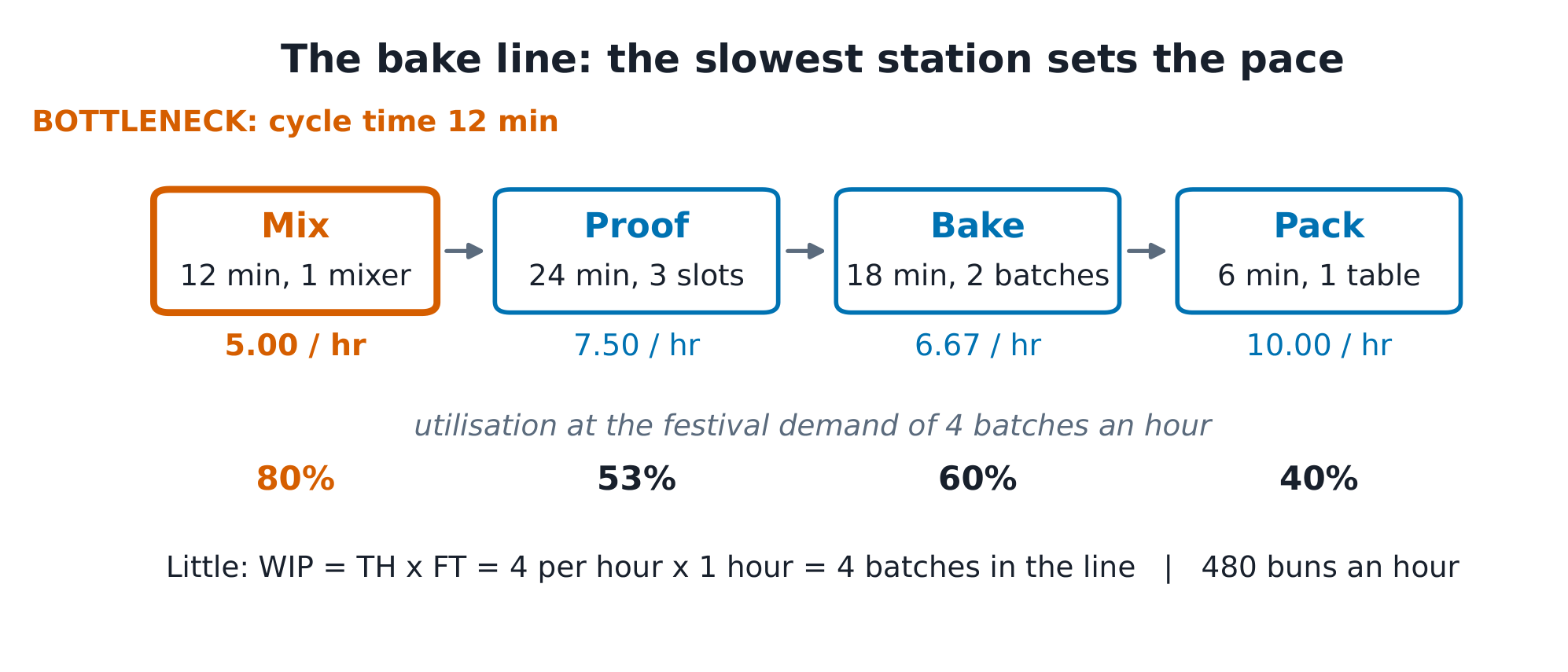
The idea, with a picture. The line: mix 12 min a batch, a three-slot prover at 24 min, a two-batch oven at 18 min, pack at 6 min. Capacities: mix 5.00 batches/hr, proof 7.50, bake 6.67, pack 10.00. The slowest — mix — is the bottleneck 瓶颈: the line runs at 5 batches = 600 buns an hour, and the cycle time 周期时间 is 12 minutes a batch.
The definitions. Throughput 产出率: the rate the line actually produces. Capacity utilisation 产能利用率 = throughput ÷ capacity. Little's law 利特尔法则: $WIP = TH \times FT$ — things in the system equal the rate through it times the time through it. Work in progress 在制品 (WIP): batches inside the line.
The derivation. Capacity per station $= 60 \times \text{slots}/t$: mix $60/12 = 5.00$; proof $60 \times 3/24 = 7.50$; bake $60 \times 2/18 = 6.67$; pack $60/6 = 10.00$. At the festival demand of 4 batches an hour, utilisations are $4/5 = 80\%$, $4/7.5 = 53.3\%$, $4/6.67 = 60.0\%$, $4/10 = 40\%$. Flow time $12 + 24 + 18 + 6 = 60$ min = 1 hr, so Little's law: $WIP = 4 \times 1 = 4$ batches ✓ — exactly what a walk down the line counts.
Worked example 1 — where an hour is won. The head baker wants to speed up packing (40% utilised). Speeding pack to 3 min moves the line nowhere: mix still caps it at 5 batches an hour. The hour is won at mix: a second mixer lifts mix to 10.00 an hour — and the bottleneck MOVES to bake (6.67), so the line gains only $6.67 - 5 = 1.67$ batches an hour (200 buns). Every investment question in operations starts the same way: where is the constraint now, and where does it move?
Worked example 2 — escalate to the Saturday surge. Festival Saturdays need 6 batches an hour for 8 hours. One mixer caps the line at 5.00: a shortfall of 1 batch an hour, 8 batches over the day. Two answers. Buy the second mixer (bake's 6.67 then clears the 6) — capital spent for one day a week. Or BAKE AHEAD: two extra hours on Friday evening at the line's 5 an hour build a buffer of $5 \times 2 = 10$ batches — inventory is rate × time, the same law — covering the 8 with two spare. Buffers are not a failure of the line; they are how a fixed line meets a moving demand, at the price of freshness, which is why the buffer is Friday's buns and not Saturday's promises.
Common mistakes. Balancing the line to raise average utilisation (instead of raising the bottleneck). Quoting capacity in buns before checking the batch size. And confusing flow time (1 hr through the process) with cycle time (12 min between outputs).
Summary. Capacity = the slowest station; cycle time is its inverse. Little's law ties WIP, throughput and flow time. Fix the constraint or buffer around it — in that order.
Quality
Why it matters. The contract's tolerance is ±10% on an 80 g bun. Weighing every bun finds bad ones; the statistical process control discipline finds the batch going bad BEFORE the buns ship.
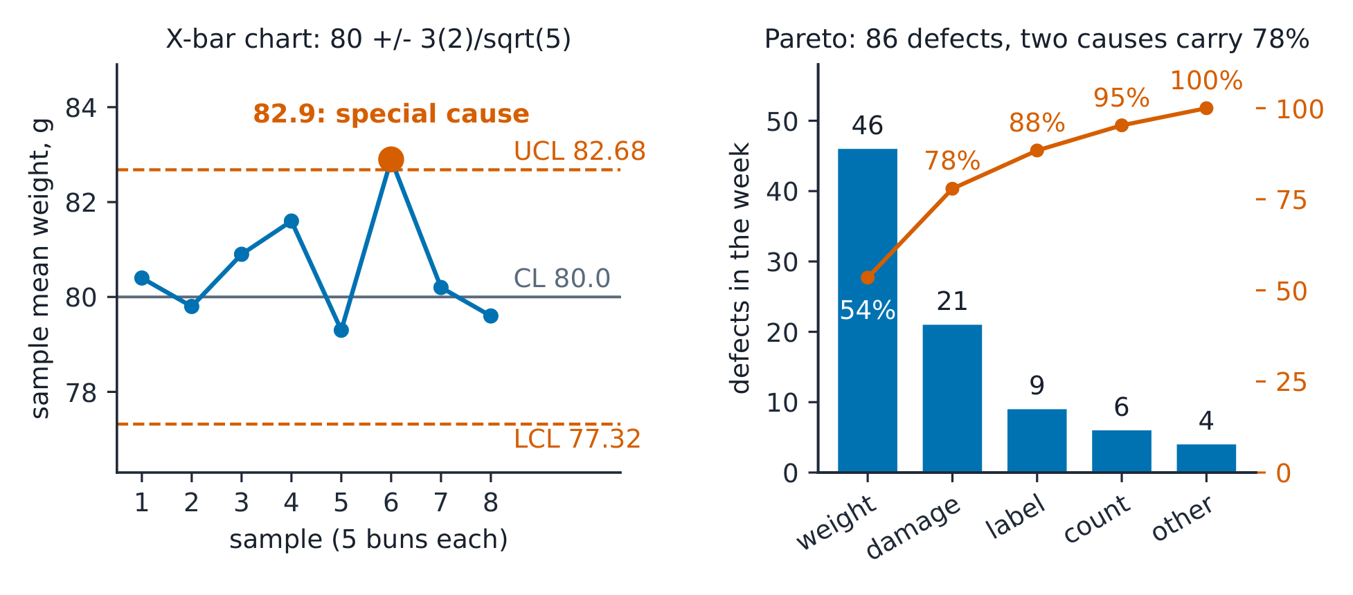
The idea, with a picture. Buns are sampled 5 at a time. With the process centred at 80.0 g and bun-to-bun sd 2.0 g, the sample-mean control chart 控制图 runs $80 \pm 3 \times 2/\sqrt{5} = 80 \pm 2.68$ g: limits 77.32 and 82.68 ✓.
The definitions. Statistical process control 统计过程控制 (SPC): steering the process, not inspecting the product. Common cause variation: the noise inside the limits. Special cause: a point beyond the limits or a run — evidence something changed. Pareto analysis 帕累托分析: rank the defects; the vital few carry most of the count. Cost of quality: prevention + appraisal + internal + external failure.
The derivation. Limits $80 \pm 3\sigma/\sqrt{n} = 80 \pm 3 \times 2/\sqrt{5} = 80 \pm 2.68$ ✓. The same limits from the range table: $\bar{R} = d_2\sigma = 2.326 \times 2 = 4.65$ g, and $A_2 \bar{R} = 0.577 \times 4.65 = 2.68$ ✓ — two routes, one answer. The R-chart's upper limit: $D_4 \bar{R} = 2.114 \times 4.65 = 9.83$ g. The week's eight means: 80.4, 79.8, 80.9, 81.6, 79.3, 82.9, 80.2, 79.6 — the sixth sits beyond 82.68 ✓ (the new flour lot), and the next week's eight means (79.4 to 79.9, all below centre for eight samples running) flag a drift by the run rule even though every point is inside the limits.
Worked example 1 — read the chart, don't nudge it. Sample 6 reads 82.9. The wrong response: retune the mixer by −0.5 g — that is tampering, adding the operator's hand to the noise (Deming's funnel). The right response: FIND the cause — the flour lot changed at that batch, its protein runs higher, water absorption shifted the dough. Fix the lot, and the chart returns to centre on its own. Within limits, leave the process alone; beyond them, look for a nameable cause.
Worked example 2 — escalate to the 19,000-pound week. The defect Pareto: underweight 46, damaged pack 21, mislabel 9, wrong count 6, other 4 (86 total; the first two carry $67/86 = 77.9\%$ ✓). The cost ledger: prevention 1,200 + appraisal 2,400 + internal failure 5,600 + external failure 9,800 = 19,000 — 19% of the week's 100,000 revenue, and failure is 81% of it. The lever the Pareto names: underweight traces to one filler head — 800 spent rebuilding it (prevention) removes 46 defects and most of the 9,800 external bill. Quality is not inspected in; it is paid for at the front, where it is cheapest.
Common mistakes. Chasing every inside-limits wiggle (tampering inflates variance). Reading the R-chart with the X-bar's limits. And reporting the defect count without the Pareto — 86 means nothing; "46 from one filler head" means Monday morning.
Summary. Limits at $3\sigma/\sqrt{n}$; a point beyond or a run is a signal with a nameable cause. Pareto ranks what to fix; the cost of quality says fix it early. Steer, don't nudge.
Inventory
Why it matters. Flour is 60% of a bun and 48,000 kg a year of the site's cash. Too little stops the line; too much is money mouldering in bins. The economic order quantity is where the two costs balance.
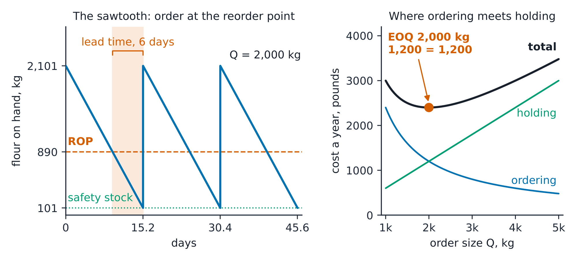
The idea, with a picture. Ordering costs £50 an order; holding costs £1.20 per kg a year. $EOQ = \sqrt{2 \times 48{,}000 \times 50/1.20} = 2{,}000$ kg ✓ — 24 orders a year, one every 15.2 days, £1,200 of ordering and £1,200 of holding, exactly equal ✓.
The definitions. Economic order quantity 经济订货批量 (EOQ): the order size minimising ordering + holding. Reorder point 再订货点 (ROP): the level that triggers an order — lead-time demand plus safety stock. Safety stock 安全库存: $z \times \sigma_{LT}$, the buffer bought for a service level. Continuous review: watch the level; periodic review: order on a clock.
The derivation. Daily demand $48{,}000/365 = 131.5$ kg; over the 6-day lead time $131.5 \times 6 = 789.0$ kg leaves the bin while the order is on the road. Demand sd 25 kg/day gives $\sigma_{LT} = 25\sqrt{6} = 61.2$; at 95% service $z = 1.645$, so safety stock = $1.645 \times 61.2 = 101$ kg ✓ and $ROP = 789 + 101 = 890$ kg ✓. At the EOQ the annual costs tie: ordering $24 \times 50 = 1{,}200$, holding $1{,}000 \times 1.20 = 1{,}200$ — the balance the square root buys.
Worked example 1 — the discount that had to be checked. The mill offers 2% off the £2.00 kg price for orders of 4,000 kg or more. The tempting answer is "2% of 96,000 — take it". The check: at 4,000 kg, purchase $48{,}000 \times 1.96 = 94{,}080$, ordering $12 \times 50 = 600$, holding $2{,}000 \times 1.20 = 2{,}400$ — total £97,080 against £98,400 at the EOQ ✓, saving 1,320 a year. But the margin is honest: the extra logistics cost is exactly 600, so the breakeven discount is $600/96{,}000 = 0.625\%$ — below that, "cheap" flour costs more than it saves. The EOQ is not always the order; it is the number every deviation must beat.
Worked example 2 — escalate to the shortage that was predictable. Festival week: demand runs 180 kg a day (37% above the 131.5 mean). The bin hits the 890 kg reorder point and an order goes out — but in the 6 days it takes to arrive the line eats $180 \times 6 = 1{,}080$ kg: a 190 kg stockout ✓, about a day of silence. The 101 kg of safety stock was sized for noise with sd 25 a day, not for an event 49 kg a day above the mean for a week. The honest reading: safety stock is the wrong tool for anything on a calendar. The operational answer is a scheduled pre-buy (one extra 1,100 kg order the week before) or a temporary periodic-review target computed from festival demand — planning, not buffering.
Common mistakes. Reordering "when the bin looks low" (no lead time). Treating the EOQ as eternal — demand moves, the square root moves. And buying a discount without the total-cost check (the 0.625% breakeven above).
Summary. $EOQ = \sqrt{2DS/H}$, where ordering = holding. ROP = lead-time demand + $z\sigma_{LT}$. Safety stock is for noise; calendars need planning, not buffers.
Forecasting
Why it matters. Every number in this course — capacity, stock, staff — is a forecast wearing a uniform. The craft is picking the method that fits the shape, and then measuring how wrong it is.
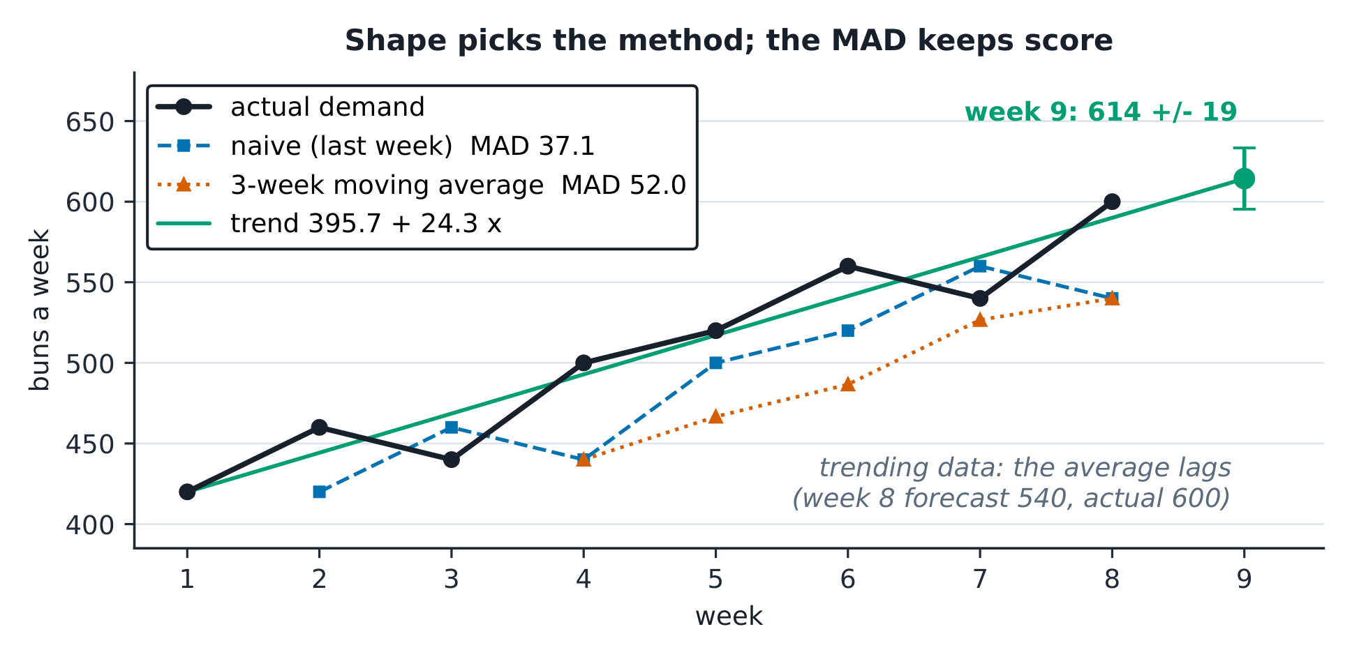
The idea, with a picture. Eight weeks of bun demand: 420, 460, 440, 500, 520, 560, 540, 600 — a rising trend. Three methods, one scoreboard: the mean absolute deviation 平均绝对误差 (MAD).
The definitions. Naive forecast: today's actual is tomorrow's forecast. Moving average 移动平均: the mean of the last $n$ weeks. Exponential smoothing 指数平滑: $F_{t+1} = F_t + \alpha e_t$ — a weighted past with fading memory. MAD = mean of $|e_t|$; divide demand by MAD to size buffers. Tracking signal = cumulative error ÷ MAD — drift past ±4 means the method has lost the process.
The derivation. Naive errors (weeks 2–8): 40, −20, 60, 20, 40, −20, 60 → MAD $260/7 = 37.1$ ✓. Three-week moving average (from week 4): 440, 466.7, 486.7, 526.7, 540 against 500, 520, 560, 540, 600 → MAD $260/5 = 52.0$ ✓. Exponential smoothing at $\alpha = 0.4$ (seed 420): forecasts 420, 436, 437.6, 462.6, 485.5, 515.3, 525.2 → MAD 48.3 ✓. The least-squares trend: $\hat{y} = 395.7 + 24.3x$; week 9 = 614 ✓ with residual sd 19.3 — so quote $614 \pm 19$ as the two-thirds band, and buy flour for the band, not the point.
Worked example 1 — the method must match the shape. The naive MAD (37.1) beats the moving average (52.0) here — not because naive is clever but because demand is TRENDING and the average drags it down (week 8: 540 forecast against 600 actual). The same moving average on flat demand would win. Method choice is not taste: fit the shape (flat → average; trend → trend model; new product → judgement), then let the MAD scoreboard arbitrate — and re-run it monthly.
Worked example 2 — escalate to the transparent adjustment. Week 9 base forecast: 614. The sales lead hears the festival added a second stage and wants "add 20%". The honest protocol: base 614 × 1.10 = 675, RECORDED as "judgemental uplift +10%, second stage, sales lead, 2026-05-04" — and at week 9 the actual 700 lands 25 above the adjusted number (3.7%), while 614 alone would have been 86 low. The lesson is not that judgement won; it is that the adjustment is written down, so next year's 614 base gets a better prior. A forecast you cannot audit is a rumour with decimals.
Common mistakes. Scoring accuracy on the wrong weeks (the moving average has no forecast for weeks 1–3 — score like with like). Letting α rise to chase noise (0.4 follows trend; 0.8 tracks weather). And hiding the judgemental uplift inside the number instead of beside it.
Summary. Shape picks the method; MAD scores it; trend data punishes averages. Forecast a band, not a point — and write every judgement beside the number it moved.
Supply chains
Why it matters. The site does not make buns; it makes buns out of a chain — mills, a bakery, two depots. Every chain choice trades cost against service against risk, and the trade is arithmetic, not slogan.
The idea, with a picture. The design question: one supplier or two, local or distant, stock at each depot or pooled centrally?
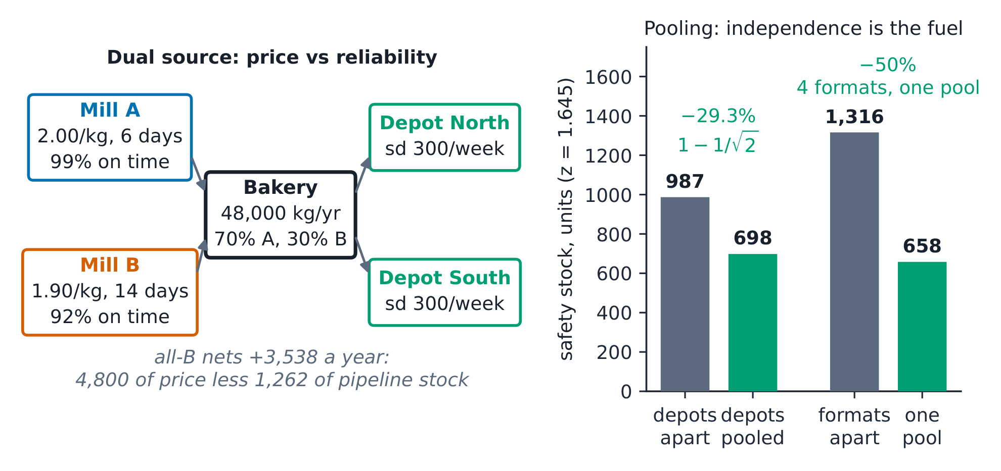
The definitions. Lead time 交货期: order to arrival. Risk pooling 风险共担: aggregate demand is less variable than its parts — $\sigma_{sum} = \sqrt{\sum \sigma_i^2}$ for independent demands (the square-root law 平方根法则). Postponement 延迟策略: hold the generic form, differentiate late. Single sourcing: cheaper, riskier; dual sourcing: the reverse.
The derivation. Each depot faces weekly demand sd 300 units (independent), one-week lead time, 95% service: each holds $1.645 \times 300 = 494$; both, 987. Pooled at one central store: $\sigma = \sqrt{300^2 + 300^2} = 424.3$, safety stock $= 1.645 \times 424.3 = 698$ — saving $987 - 698 = 289$, exactly $1 - 1/\sqrt{2} = 29.3\%$ ✓. The same law prices postponement: four pack formats each needing 1,316 units of finished safety stock ($4 \times 1.645 \times 200$) can be held as one generic pool of $1.645 \times 400 = 658$ — half ✓.
Worked example 1 — the cheap mill that wasn't cheap. Mill B bids £1.90 against A's £2.00 — saving $0.10 \times 48{,}000 = £4{,}800$ a year. But B is a 14-day lead against A's 6, so 8 extra days of pipeline stock, $8 \times 131.5 = 1{,}052$ kg at £1.20 to hold = £1,262 — the net is still +£3,538 ✓. The arithmetic says yes; the RISK column says read on: B delivers on time 92% of the time against A's 99%, single-sourced, harvest-exposed. One missed 14-day delivery is a stopped line (the site holds 1,052 kg — 8 days; a second miss is closure). The decision: dual-source, 70% A for reliability, 30% B for price and leverage. The number never decides alone; it prices the menu.
Worked example 2 — escalate to the postponed bun. Four pack formats (plain 40%, seeded 30%, branded festival 20%, gluten-free 10%) each carry their own forecast error. Label-and-pack at the depot instead of the bakery: the bakery ships generic buns (one forecast, sd 400) and differentiation happens after demand is visible — safety stock halves from 1,316 to 658 ✓, and the gluten-free format stops being baked to a two-week-old guess. The cost of postponement is real — a depot packing line at £18,000 — so it is checked like every other number in this course: write-offs fall with the safety stock, about 600 buns a week at £0.50 = £300 a week, £15,600 a year, so the line pays back in 14 months ✓. Postponement is the pooling law in time instead of space.
Common mistakes. Adding supplier standard deviations (variances add; the square root does the work). Sourcing on price alone after the pipeline-stock check says otherwise. And calling a chain "resilient" with no number — resilience is measured in days of coverage and per cent on-time.
Summary. $\sigma_{sum} = \sqrt{\sum\sigma_i^2}$: pooling and postponement both live on independence. Lead time is inventory in disguise. Cost, service, risk — price all three, then choose.
Project management
Why it matters. The second site was built in 18 days of planned work — and the plan, the crash and the cost tracking are three disciplines that keep a project from being a story told afterwards.
The idea, with a picture. The fit-out as activities: A design sign-off 2 d, B strip-out 3, C electrical rewire 5, D oven install 4, E ventilation 4, F decor 3, G equipment test 2, H handover 1. The critical path A-B-C-D-F-H totals 18 days ✓; E floats 5 days, G floats 1.
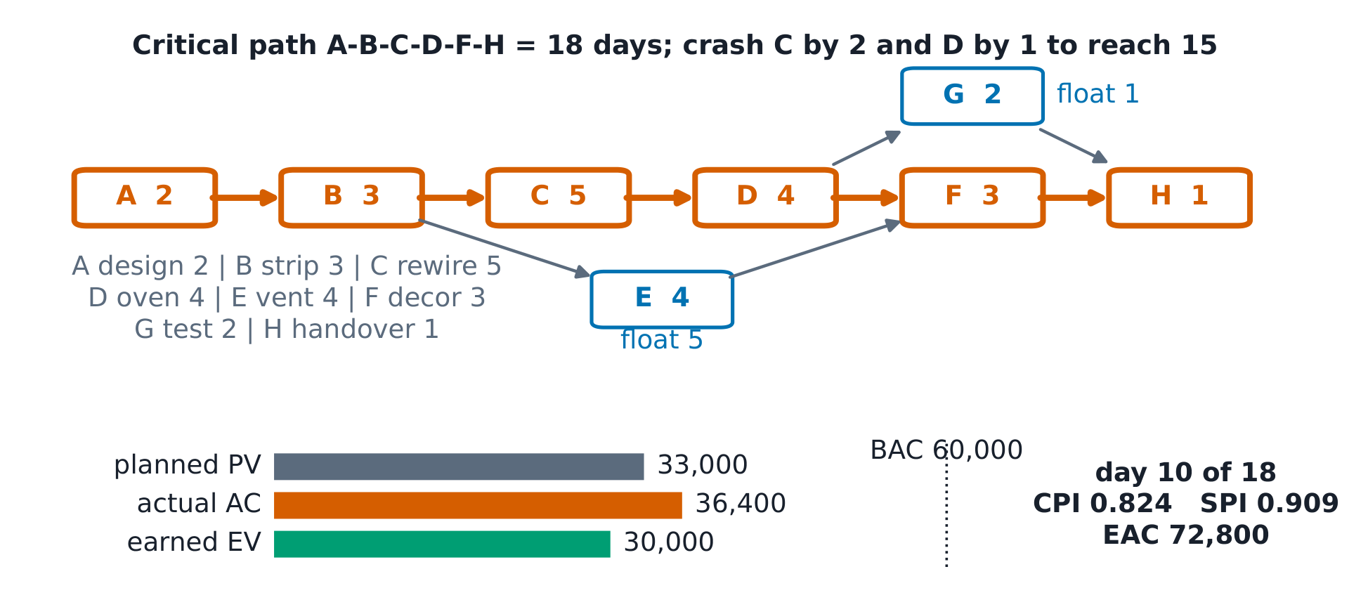
The definitions. Critical path 关键路径: the longest path; float zero on every activity. Total float 总时差: how late an activity can start without delaying the project. Crashing 赶工: buying time on the critical path at a cost per day. Earned value analysis 挣值分析: $CPI = EV/AC$, $SPI = EV/PV$ — cost and schedule health in two ratios.
The derivation. Forward pass: ES of H = 18; backward pass gives E float $14 - 9 = 5$ and G float $17 - 16 = 1$, everything on A-B-C-D-F-H zero ✓. Crashing: C can compress 2 days at £400/day (overtime), D one day at £600/day (crew); a day saved is worth £700 (the festival deadline). Crash C by 2: 16 days, cost 800 against 1,400 of value; the near-critical path A-B-C-D-G-H is now 15, so crashing D one more day pulls both to 15 — cost 600 against 700 ✓. Total: 18 → 15 days for £1,400 of crash against £2,100 of value, net +£700 ✓, and E's float absorbs the noise.
Worked example 1 — the float is not yours. The ventilation contractor asks to start E five days late to fit another job — "it has 5 days of float, nothing moves". Arithmetically true today; the error is ownership. Float belongs to the PROJECT, not the trade: spend it on E and a later surprise elsewhere has nowhere to go. When the decor crew (F) is then held two days by late paint, F's slip lands straight on the end date, where before it would have been absorbed by moving F after an on-time E. The discipline: float is a shock absorber managed by the project manager, released to a trade only in writing, with the end date recomputed the same day.
Worked example 2 — escalate to the earned-value audit. Budget at completion £60,000 (the raise of course 9). Day 10 of 18: planned value 33,000, actual cost 36,400, earned value 30,000 (half the scope done). $CPI = 30{,}000/36{,}400 = 0.824$ ✓ and $SPI = 30{,}000/33{,}000 = 0.909$ ✓: 82p of value earned per pound spent, 9% behind schedule. $EAC = BAC/CPI = 60{,}000/0.824 = £72{,}800$ ✓ — a £12,800 overrun flagged on day 10, while it is still a management problem, not a post-mortem. The naive reading ("we spent 36,400 of 60,000, 61% through the money") hides that only 50% of the VALUE is earned. The two-ratio discipline says what is wrong, where, and early.
Common mistakes. Crashing the cheapest activity instead of the critical one (money spent off the path buys nothing). Letting trades consume float. And tracking cost without EV — spend is not progress.
Summary. The critical path is the project; float is a shared shock absorber. Crash where the path runs, at a price below the day's value. $CPI$ and $SPI$ flag overruns while they are still decisions.
Sustainability in operations
Why it matters. The festival's sponsor wants "a carbon-neutral bun". Whether the claim survives arithmetic depends entirely on where the boundary is drawn — and unstated boundaries are how greenwash is manufactured.
The idea, with a picture. The site's own operation (gate-to-gate) runs at 2,492 kg CO2e a week ✓: electricity 9,600 kWh × 0.19 = 1,824, gas 3,200 × 0.18 = 576, deliveries 420 km × 0.22 = 92. Draw the boundary one step wider and flour adds 508 kg — 20% more, from one input.
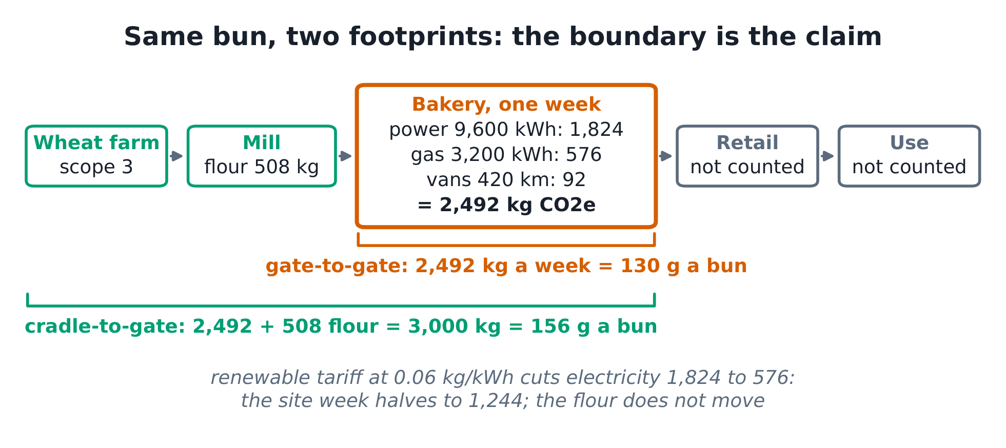
The definitions. Carbon footprint 碳足迹: CO2e emitted within a stated system boundary 系统边界. Gate-to-gate: the site's own operation. Cradle-to-gate: plus everything upstream. Scope 1 (direct fuel), Scope 2 (purchased electricity), Scope 3 (everything else in the chain). Circularity: keeping materials in use — reuse beats recycle beats dispose.
The derivation. Weekly energy: $9{,}600 \times 0.19 = 1{,}824$; $3{,}200 \times 0.18 = 576$; $420 \times 0.22 = 92.4$ — total $2{,}492$ kg ✓, which is $2{,}492/19{,}200 = 130$ g per bun ✓. Upstream flour at 0.55 kg CO2e per kg and 923 kg a week adds 508 kg, so cradle-to-gate is $2{,}492 + 508 = 3{,}000$ kg — and the boundary, not the bun, decided the 20% jump. On a renewable tariff at 0.06 kg/kWh, electricity falls 1,824 → 576 and the site's own footprint halves (2,492 → 1,244, a 50% fall; 42% cradle-to-gate) with no operational change at all — the same fact that makes the claim honest makes it cheap to game, which is why the tariff must be additional, not a certificate shuffle.
Worked example 1 — the tray that pays only if it comes back. Cardboard trays: 42,000 a year at £0.22 = £9,240, six tonnes of board, 4.2 t CO2e upstream. The circular alternative: returnable trays at £5.50, a two-week cycle, so a pool of $808 \times 2 = 1{,}616$ trays (£8,888). The whole decision is the return rate. At 98% returns the site loses 840 trays a year (£4,620) and washes 42,000 (£1,470): running cost £6,090, saving £3,150 a year, payback 2.8 years ✓. At 95% returns, losses alone cost £11,550 and the scheme LOSES £3,780 a year ✓. Breakeven return rate: 96.6% ✓. Emissions at 98%, amortised honestly: the pool spread over a five-year life (323 a year) plus 840 losses = 1,163 trays a year × 0.6 kg × 3.0 kg CO2e per kg = 2,093 kg, plus 300 kg of wash energy = 2.4 t against 4.2 t — a 43% cut ✓, but only with the pool's manufacture, the losses and the wash INSIDE the boundary. Circularity claims with no loss rate are decoration.
Worked example 2 — escalate to the neutral bun. The sponsor's claim, audited: cradle-to-gate 3,000 kg for the site's 19,200 buns a week = 156 g a bun ✓; add the retail stage and the customer's drive and it only climbs — no boundary makes the bun neutral. What survives scrutiny is a REDUCED claim with the boundary stated: "156 g a bun cradle-to-gate, week-41 audit, renewable tariff and tray pool in place, boundary excludes retail and use". The operations answer to greenwash is always the same shape: a number, a boundary, a date, and something the competition can verify. "Neutral" without those four is a word, not a fact.
Common mistakes. Comparing footprints with different boundaries (the 2,492 vs 3,000 trick is the standard one). Offsetting Scope 2 while Scope 3 dwarfs it. And treating circularity as free — every reuse loop has a wash, a reverse logistics leg, and a loss rate, all inside the boundary.
Summary. The boundary IS the claim: state it, then measure inside it. Scope 2 moves with the tariff; Scope 3 needs the chain. Circularity pays when the loop's costs stay inside it.
The project sheet (reproducible)
Second-site bake line, festival contract:
- Line: mix 12 min / proof 24 (×3) / bake 18 (×2) / pack 6 → capacities 5.00 / 7.50 / 6.67 / 10.00 batches an hour; bottleneck mix, cycle time 12 min. At 4 batches an hour: utilisations 80 / 53.3 / 60 / 40%. Little: WIP 4 = 4 × 1 hr. 480 buns an hour; 19,200 a week.
- Quality: X-bar $80 \pm 2.68$ → [77.32, 82.68]; $\bar{R} = 4.65$, R-chart UCL 9.83; sample 6 at 82.9 = special cause; Pareto 46/21/ 9/6/4 (77.9% in two); COQ 19,000 = 19% of sales, 81% failure.
- Inventory: EOQ $\sqrt{2 \times 48{,}000 \times 50/1.20} = 2{,}000$ kg; 24 orders, 15.2-day cycle; £1,200 = £1,200. ROP = 789 + 101 = 890 kg ($z = 1.645$, $\sigma_{LT} = 61.2$). Discount check: 2% at 4,000 kg saves 1,320; breakeven 0.625%.
- Forecast: 420→600 over 8 weeks; MAD naive 37.1 / MA3 52.0 / ES(0.4) 48.3; trend $\hat{y} = 395.7 + 24.3x$; week 9 = 614 ± 19.
- Chain: mill B nets +3,538 but 92% on-time single-sourced → dual 70/30. Pooling: 987 → 698 (29.3% = $1 - 1/\sqrt2$); postponement 1,316 → 658 (half).
- Project: A-B 2-3, C-D 5-4, E 4, F 3, G 2, H 1 → critical path A-B-C-D-F-H = 18 d; floats E 5, G 1; crash C −2 and D −1 → 15 d, +£700 net. EVM day 10: PV 33,000, AC 36,400, EV 30,000 → CPI 0.824, SPI 0.909, EAC 72,800.
- Footprint: gate-to-gate 2,492 kg/wk (1,824 + 576 + 92); 130 g/bun; cradle-to-gate 3,000 kg (flour +508); renewable tariff: site 2,492 → 1,244 (−50%), cradle-to-gate −42%.
Every figure in this handout recomputes from these values.