A number needs a method
Two groups measure the same wire. Their values differ. Which should you trust? You need more than the final number: the instrument, method, repeated readings and uncertainty all matter.
WPH13 Practical Skills in Physics I is a written paper about practical work from Units 1–2. It lasts 80 minutes and has 50 marks. All questions are compulsory. At least 20 marks assess mathematics at Level 2 or above. This guide supports real laboratory work; reading it does not replace making measurements yourself.
The three skill sheets follow the process: plan a valid investigation, collect and record measurements, then process results and justify conclusions. The official specification gives skill lists rather than numbered knowledge statements for this unit.
Planning a valid investigation
A valid measurement 有效测量 measures what you intend to measure. A precise timer does not help if it times the wrong event.
Start by naming the independent variable 自变量 that you change and the dependent variable 因变量 that you measure. List control variables 控制变量 that could also affect the dependent variable. Say how you will keep each important one steady.
Turn a description into a usable method
A method needs:
- named apparatus, with a suitable measuring range and resolution 分辨率;
- an arrangement showing where measurements are taken;
- steps that another student can follow, including the start and end events;
- several independent-variable settings over a useful range;
- repeats where they test stability and estimate variation;
- a calculation or graph that answers the investigation question;
- specific sources of uncertainty and improvements;
- realistic hazards with a practical way to reduce each risk.
Do not write only “take readings” or “use better equipment”. Name the reading, the instrument and what the improvement changes.
Worked planning example: string frequency and tension
Investigate how fundamental frequency depends on tension in a string.
- Use a vibration generator and signal generator. Pass the string over a pulley to a mass hanger.
- Change hanging mass $m$. With a freely moving pulley, tension is approximately $T=mg$.
- Measure vibrating length between the end nodes. Use the same string and keep that length fixed.
- Adjust frequency for the fundamental each time. The same mode is a control, not an optional detail.
- Measure the string's mass and total length to find linear density $\mu$. Keep it unchanged in this investigation.
- Record several tensions and their resonant frequencies. Repeat the tuning near each resonance.
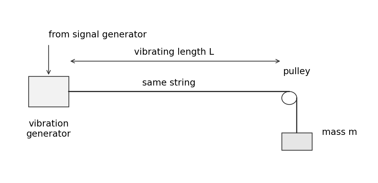
The model for the fundamental is:
A graph of $f^2$ vertically against $T$ horizontally should be straight through the origin. A large triangle gives the gradient. Secure the stand and keep your feet away from falling masses. This is stronger than saying “be careful”.
Calibration and zero checks
Calibration 校准 checks an instrument against known reference values. A zero error 零点误差 occurs when it does not read zero at the correct zero condition. Check closed micrometer jaws or an empty balance before measuring.
If a micrometer reads $+0.03\ \text{mm}$ with its jaws correctly closed, subtract $0.03\ \text{mm}$ from each subsequent reading. Repeating the measurement alone does not remove that offset. A zero check cannot prove that every point on the scale is calibrated correctly.
Range, spacing and repeats
Choose a range wide enough to reveal the relationship. Several measurements crowded near one setting may give a poor gradient. Use more settings near a turning point if you need to locate a maximum accurately.
Repeats are useful when conditions can be reproduced. They show scatter and help identify unstable readings. However, repeated readings of a discharging cell or a heating wire may drift because the conditions change. Reduce the current, switch off between readings, control temperature or restore conditions. Do not average a drift as though it were random variation.
Control the actual cause
When varying the angle of a lamp above a solar cell, keep lamp–cell distance and lamp output fixed. Control background light, for example with shielding or a darkened room. Keep the cell and its load the same. Otherwise a change in measured power may come from distance, illumination or circuit resistance instead of angle.
Discuss context using a physical cause. A tracking solar panel can stay closer to normal incidence and collect more energy over a day. Its motor also uses energy and adds cost or maintenance. “Better for the environment” alone does not explain either effect.
Measuring and recording
Accuracy 准确度 describes closeness to the true value. Precision 精密度 describes how closely repeated values cluster. Closely clustered results can still all share a systematic offset.
- Repeatability 重复性 concerns similar results using the same operator and method over a short time.
- Reproducibility 再现性 concerns similar results from different operators, apparatus or methods.
- Random effects 随机影响 cause unpredictable variation. Repeating and taking a mean can reduce their influence.
- Systematic error 系统误差 shifts results in a consistent way. Correct the cause or known offset; repeating does not remove it.
- Uncertainty 不确定度 is a reasonable interval associated with a measurement. It is not automatically a mistake or the known size of the error.
Read instruments at their resolution
A millimetre ruler has a smallest interval of $1\ \text{mm}$. The specification's standard Vernier calipers resolve $0.1\ \text{mm}$, and its standard micrometer resolves $0.01\ \text{mm}$. Check the instrument shown: a digital display or a different scale may have a different resolution.
For a micrometer, add the visible sleeve reading and the thimble reading. Include a visible half-millimetre sleeve mark when appropriate. Use the ratchet for consistent contact pressure, rather than overtightening the jaws.
For Vernier calipers, read the main scale just before the Vernier zero, then add the aligned Vernier division times its resolution. Check that the jaws contact the intended surfaces without tilting. Do not infer a missing scale from an extracted text description: read the instrument diagram itself.
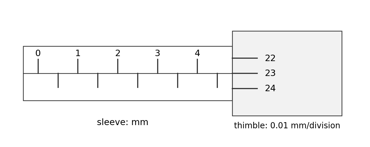
Worked example. The last visible sleeve mark is $4.5\ \text{mm}$. Thimble division 23 aligns with the reference line. Resolution is $0.01\ \text{mm}$ and zero error is $+0.02\ \text{mm}$.
Geometry and timing techniques
Avoid parallax 视差 by viewing a scale along the correct line of sight. Use a set square to transfer a height or position onto a ruler. Keep the ruler parallel to the distance being measured; a sloping ruler measures a different distance.
A light gate measures the blocking time of an interrupting object. With known interrupting length $l$, speed is $v=l/t$. That gives speed during passage, not acceleration by itself. To find acceleration, measure a change of speed over known time, or use a justified motion equation with additional measured quantities. Do not call $l/t$ acceleration.
A video with known frame rate can reduce reaction-time uncertainty. Count frames between clearly defined start and end events, then use $t=N/f_{\text{frame}}$. The frame interval limits timing resolution. Blurred images or unclear event positions can still limit the result.
Tables and significant figures
Put quantity and unit together in each column heading, for example $l/\text{mm}$. Record raw measurements with decimal places matching instrument resolution. Do not add extra digits that the instrument cannot resolve.
| Reading | Time / s |
|---|---|
| 1 | 5.12 |
| 2 | 5.24 |
| 3 | 5.18 |
| 4 | 5.20 |
These all have the same two decimal places. A calculated mean can be kept with extra digits during working, then reported sensibly. Processed values for plotting are commonly given to three significant figures, unless the question or data requires otherwise. Do not mix $5.1$, $5.24$ and $5.180$ as if they came from one unchanged display.
An anomalous reading 异常读数 does not fit the pattern. Check the reading, method and repeat measurement if possible. Do not silently delete the least convenient value. A suspected anomaly needs a reason and a recorded decision.
Uncertainty in this unit
For one reading, this specification uses half the instrument resolution as the basic absolute uncertainty estimate. This does not mean resolution is the only source of uncertainty. A poorly defined endpoint, reaction time or alignment may make the uncertainty larger.
Worked example. A balance displays $135.0\ \text{g}$ with resolution $0.1\ \text{g}$.
For repeated values, the specification uses half range 半极差 as an uncertainty estimate:
Worked example. Repeated times are $5.12$, $5.24$, $5.18$, $5.20\ \text{s}$.
Report about $(5.19\pm0.06)\ \text{s}$. Keep the unrounded mean in the percentage calculation. The repeat spread is much larger than half a hundredth of a second, so quoting display resolution alone would miss the observed variation.
Unit 3 does not require compounding percentage uncertainties in a calculated quantity. If an uncertainty for that quantity is supplied, use it directly. Do not introduce an advanced propagation rule as a requirement here.
Graphs and processing results
Choose scales that show the data
Read which quantity belongs on each axis. Use clear quantity/unit labels and regular scales. Use a large part of the available grid; avoid awkward intervals that are hard to subdivide. Neither axis must always start at zero, but do not hide whether a proposed proportional relationship passes through the origin.
Plot small crosses accurately. Draw a thin best-fit line or smooth curve according to the relationship. Do not join noisy points with a zigzag unless the question requests it. A best-fit straight line balances scatter rather than passing through every point.
Turn a gradient into a physical constant
For a line $y=mx+c$, identify which part of the physical equation matches $m$ and $c$. A straight line does not prove direct proportionality if its intercept is non-zero.
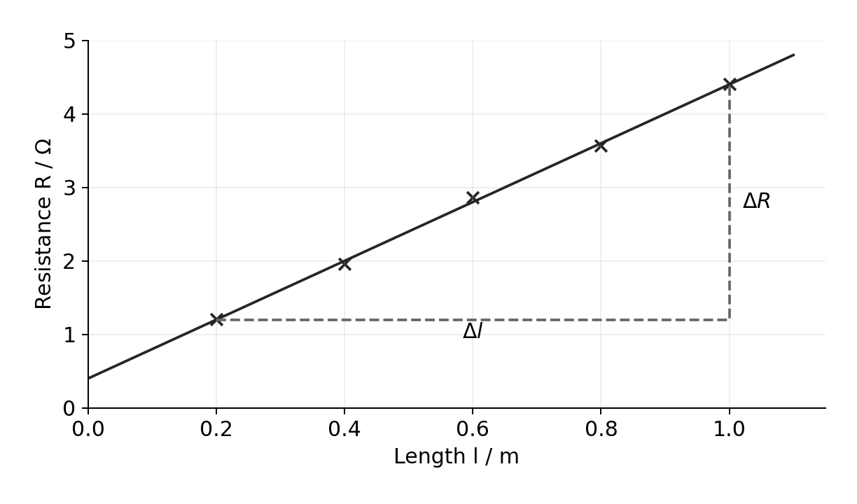
Worked example. A wire follows $R=(\rho/A)l+R_0$. A best-fit line passes through $(0.20\ \text{m},1.20\ \Omega)$ and $(1.00\ \text{m},4.40\ \Omega)$.
- Known: two widely separated points on the fitted line. Why: the slope equals $\rho/A$.
$$m = \frac{\Delta R}{\Delta l} = \frac{4.40-1.20}{1.00-0.20}\ \Omega\,\text{m}^{-1} = 4.00\ \Omega\,\text{m}^{-1}$$$$R_0 = R-ml = 1.20\ \Omega-4.00\ \Omega\,\text{m}^{-1}\times0.20\ \text{m} = 0.40\ \Omega$$
If $A=1.0\times10^{-7}\ \text{m}^2$, the resistivity is:
The fixed intercept may represent contact or lead resistance. Dividing one measured $R$ by $l$ would include that offset and give the wrong slope.
Scale factors belong in the gradient
Suppose an axis is labelled $f/\text{MHz}$. A gradient read from that graph has MHz in its units. Convert to Hz before using SI constants. A graph of $f$ against $\sin\theta$ has a dimensionless horizontal axis; its gradient therefore has frequency units. Use degree mode if the measured angle is in degrees.
If a supplied equation is $f=(v/\lambda)\sin\theta$, a graph of $f$ against $\sin\theta$ has gradient $v/\lambda$. Rearrange $v=\lambda\times\text{gradient}$. Do not assume every frequency graph has gradient equal to speed.
Curves, maxima and specific improvements
A broad range first locates a maximum. Then take more closely spaced readings around that region. Repeating one point does not locate the maximum between existing points. Keep the other conditions steady, and consider scatter when quoting the best angle or resistance.
For a motion experiment, a set square can improve a horizontal-distance measurement. For a lamp experiment, a dark enclosure can reduce changing background illumination. For a resonance experiment, approach the loudest sound from both higher and lower frequencies and repeat. Each improvement targets a named limitation.
Conclusions supported by uncertainty
A value with uncertainty describes an interval. Compare that interval with the proposed value, then state what the evidence supports. Agreement within uncertainty does not prove that a material or model is uniquely identified.
Worked example. A measured density is $8.90\ \text{g cm}^{-3}$ with percentage uncertainty $0.9\%$. Could it agree with a proposed value $8.94\ \text{g cm}^{-3}$?
The interval is about $8.82$ to $8.98\ \text{g cm}^{-3}$. The proposed value lies inside it, so the measurement is consistent with that value. It does not prove the object has that composition.
If two model predictions both lie inside the interval, the data does not distinguish them. Reduce the dominant uncertainty or add a different measurement before claiming a unique identification.
Check yourself
Before attempting a written practical problem, check that you can:
- turn apparatus names into a usable method with controls and a processing route;
- read resolution and correct a known zero offset;
- distinguish accuracy, precision, repeatability and reproducibility;
- calculate a mean, half range and percentage uncertainty;
- plot data, use a large gradient triangle and interpret an intercept;
- turn a supplied uncertainty into an interval and give a justified conclusion;
- link each improvement to the measurement problem it actually reduces.