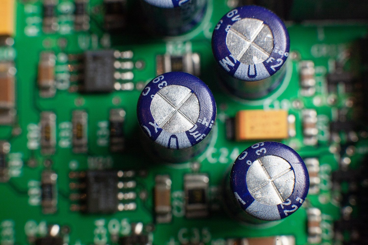
انظر عن قرب إلى فلاش الكاميرا. قبل التقاط الصورة، جزء صغير يزمجر ويصيح لمدة ثانية — ربما تسمعه حتى. إنه يشحن مكثفاً، مخزناً…
English narration · English + 中文 subtitles burned in · سرد باللغة الإنجليزية · ترجمة مدمجة بالإنجليزية + الصينية
19.1
Capacitance · السعة الكهربائية
Syllabus · المنهج
English
define capacitance, as applied to both isolated spherical conductors and to parallel plate capacitors
recall and use $C = Q/V$
derive, using $C = Q/V$, formulae for the combined capacitance of capacitors in series and in parallel
use the capacitance formulae for capacitors in series and in parallel
العربية
عرّف السعة الكهربائية، كما تنطبق على الموصلات الكروية المعزولة والمكثفات ذات الصفائح المتوازية
استرجاع واستخدام $C = Q/V$
اشتق، باستخدام $C = Q/V$، الصيغ الرياضية لـالسعة المكافئة للمكثفات الموصلة على التوالي وعلى التوازي
استخدم صيغ السعة الكهربائية للمكثفات الموصلة على التوالي وعلى التوازي
Source: Cambridge International syllabus · المصدر: منهج كامبريدج الدولي
English
A capacitor 电容器 stores charge. The simplest one is two parallel conductor 导体 plates with an insulator 绝缘体 (a dielectric 电介质, or just vacuum 真空 / air) between them. Connected to a battery, charge $+Q$ builds up on one plate and $-Q$ on the other, with a potential difference 电势差$V$ across the gap.
How the plates become charged. Connect the plates to a battery and electrons flow, through the battery, from the plate joined to the positive terminal 接线端 to the plate joined to the negative terminal. One plate is left with charge $+Q$ and the other gains $-Q$: the charges are always equal and opposite, so the capacitor as a whole stays neutral. The flow stops when the p.d. between the plates equals the e.m.f. of the battery. Nothing crosses the gap; the insulator is what keeps the charge separated.
The capacitance 电容$C$ of any capacitor (or any isolated conductor) is
$$C = \frac{Q}{V}.$$
This applies to:
an isolated sphere holding charge $Q$ at potential $V$ (zero at infinity). For radius $r$, $V = Q/(4\pi\varepsilon_{0}r)$, so $C = 4\pi\varepsilon_{0} r$.
a parallel-plate capacitor: charges $\pm Q$ on the plates, p.d. $V$ between them.
Unit: farad 法拉 (F) $= \text{C V}^{-1}$. A farad is huge, so real capacitors run from $\text{pF}$ to $\text{mF}$.
Capacitance is constant for a given capacitor (set by its size and dielectric). Doubling the charge doubles the voltage, so $C = Q/V$ stays the same.
The two-mark definitions. For a parallel-plate capacitor: the charge on one plate per unit potential difference between the plates. For an isolated sphere (or any isolated conductor): the charge on the conductor per unit potential. The examiner looks for "charge per unit p.d." (or "per unit potential") and, for the plates, that the charge is the charge on one plate and the p.d. is that between the plates. "The charge stored" is accepted; "the total charge on both plates" is not, because that total is zero.
What sets the capacitance. For parallel plates the capacitance is proportional to the plate area and inversely proportional to the separation$x$ ($C \propto 1/x$: halve the gap and the capacitance doubles), and it rises when a dielectric replaces the air. A question that states "$C$ is inversely proportional to $x$" and then moves the plates apart at constant charge is asking for $V = Q/C \propto x$: the p.d. rises in proportion. At constant p.d. (still connected to the supply) it is the charge that falls instead.
Worked example. A $100\ \mu\text{F}$ capacitor is charged to $12\ \text{V}$. Find the charge stored.
Worked example. An isolated metal sphere of radius $15\ \text{cm}$ is charged to a potential of $9.0 \times 10^{3}\ \text{V}$. Find its capacitance and its charge. It is then discharged to earth through a $120\ \text{M}\Omega$ resistor: find the time constant of the discharge.
The time constant is $RC = (1.2 \times 10^{8})(1.67 \times 10^{-11}) = 2.0 \times 10^{-3}\ \text{s}$: even through an enormous resistance the sphere loses its charge in milliseconds, because its capacitance is so small. Notice that $4\pi\varepsilon_{0} = 1/(8.99 \times 10^{9})$, so $C = r/(8.99 \times 10^{9})$ with $r$ in metres.
Combining capacitors
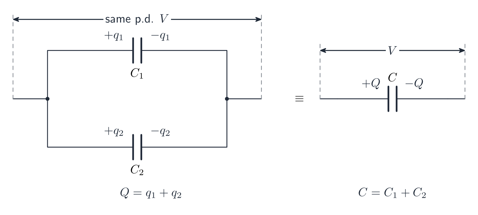
Capacitors in parallel share the same p.d. $V$. The total charge is the sum:
$$Q_{\text{total}} = C_{1} V + C_{2} V + \ldots, \qquad\text{so}\qquad C_{\text{parallel}} = C_{1} + C_{2} + \ldots$$
A parallel combination has larger capacitance than any one capacitor.
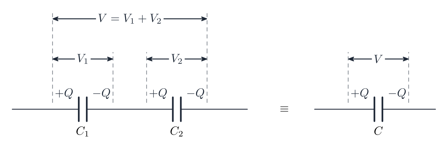
Capacitors in series carry the same charge$Q$. The total p.d. is the sum:
A series combination has smaller capacitance than any one capacitor.
Note: these rules are the opposite of those for resistors (resistors sum in series; capacitors sum in parallel), because $C = Q/V$ has $V$ on the bottom while $R = V/I$ has $I$ on the bottom.
Deriving the two rules
"Derive an expression for the combined capacitance" is a show that question, and the mark scheme wants the physics stated, not just the algebra.
Series. The capacitors carry the same charge$Q$: the plate joined to the positive terminal loses electrons to the far plate of the next capacitor, so every plate in the chain holds $\pm Q$. The p.d.s add: $V = V_{1} + V_{2}$. With $V_{1} = Q/C_{1}$ and $V_{2} = Q/C_{2}$, and the combination defined by $V = Q/C$, dividing through by $Q$ gives $1/C = 1/C_{1} + 1/C_{2}$.
Parallel. The capacitors have the same p.d.$V$, because each is connected directly across the supply. The charges add: $Q = Q_{1} + Q_{2} = C_{1}V + C_{2}V$, and $Q = CV$ for the combination, so $C = C_{1} + C_{2}$.
Two capacitors in series always give less than the smaller one; two equal capacitors $C$ give $C/2$ in series and $2C$ in parallel.
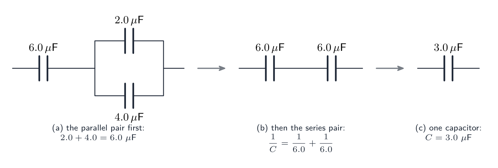
Worked example. A $6.0\ \mu\text{F}$ capacitor is in series with a parallel pair of $2.0\ \mu\text{F}$ and $4.0\ \mu\text{F}$. Find the total capacitance, and the charge on each capacitor when $12\ \text{V}$ is applied across the network.
Parallel pair: $2.0 + 4.0 = 6.0\ \mu\text{F}$. In series with $6.0\ \mu\text{F}$: $1/C = 1/6.0 + 1/6.0$, so $C = 3.0\ \mu\text{F}$. Total charge $Q = CV = (3.0 \times 10^{-6})(12) = 3.6 \times 10^{-5}\ \text{C}$: this is the charge on the $6.0\ \mu\text{F}$ capacitor (series, same charge), and it is shared by the parallel pair in the ratio of their capacitances (same p.d., $6.0\ \text{V}$ across each): the $2.0\ \mu\text{F}$ holds $1.2 \times 10^{-5}\ \text{C}$ and the $4.0\ \mu\text{F}$ holds $2.4 \times 10^{-5}\ \text{C}$. Check: they add to $3.6 \times 10^{-5}\ \text{C}$.
Worked example. Capacitors X and Y, each of capacitance $C$, are connected in series across a supply of voltage $V$; capacitors P and Q, each $C$, are connected in parallel across an identical supply. Compare the charge drawn from each supply and the energy stored in each arrangement.
Series: $C_{\text{s}} = C/2$, charge $Q_{\text{s}} = CV/2$, energy $\tfrac{1}{2} C_{\text{s}} V^{2} = CV^{2}/4$. Parallel: $C_{\text{p}} = 2C$, charge $2CV$, energy $CV^{2}$. The parallel arrangement draws four times the charge and stores four times the energy, because at the same supply voltage the energy is $\tfrac{1}{2} C V^{2}$ and the capacitance is four times larger. Asked which arrangement stores more energy from a given supply, the answer is always parallel.
العربية
تخزن المكثفات الشحنة الكهربائية في الدائرة.
يخزن الـ مكثف الشحنة. أبسط شكل هو صفيحتان متوازيتان من موصل بينهما عازل (عزل كهربائي، أو فاقد / هواء). عند توصيله ببطارية، تتراكم شحنة $+Q$ على إحدى الصفيحتين وشحنة $-Q$ على الأخرى، مع وجود فرق جهد$V$ عبر الفاصل.
مكثف صفيحتين متوازيتين: شحنات متساوية ومعاكسة على صفيحتين مع فرق جهد $V$ عبر الفاصل
كيف تتشح الصفائح. قم بتوصيل الصفائح بمصدر جهد وتتحرك الإلكترونات، عبر المصدر، من الصصلة الموصولة بالطرف الموجب الموجب إلى الصصلة الموصولة بالطرف السالب. تترك إحداهما بشحنة $+Q$ والأخرى تكتسب $-Q$: الشحنات دائماً متساوية ومعاكسة، لذا يبقى المكثف ككل متعادلاً. يتوقف التدفق عندما يساوي فرق الجهد بين الصفائح القوة الدافعة الكهربائية للمصدر. لا شيء يعبر الفجوة؛ العازل هو ما يحافظ على فصل الشحنات.
السعة الكهربائية $C$ لأي مكثف (أو أي موصل معزول) تُعطى بالعلاقة:
$$C = \frac{Q}{V}.$$
تُطبق هذه العلاقة على:
كرة معزولة تحمل شحنة $Q$ عند جهد $V$ (صفر عند اللانهاية). لنصف قطر $r$، تكون $V = Q/(4\pi\varepsilon_{0}r)$، وبالتالي $C = 4\pi\varepsilon_{0} r$.
مكثف صفيحتين متوازيتين: شحنة $\pm Q$ على الصفيحتين، فرق جهد $V$ بينهما.
الوحدة: فاراد (F) $= \text{C V}^{-1}$. الفاراد كبير جداً، لذا تعمل المكثفات الحقيقية من $\text{pF}$ إلى $\text{mF}$.
السعة ثابتة لمكثف معين (تحدها أبعاده والديLocated). مضاعفة الشحنة تضاعف الجهد، لذا يظل $C = Q/V$ ثابتاً.
تعريفات العلامتين. بالنسبة لـمكثف صفيحتين متوازيتين: الشحنة الموجودة على صفيحة واحدة لكل وحدة فرق جهد بين الصفيحتين. بالنسبة لـكرة معزولة (أو أي موصل معزول): الشحنة الموجودة على الموصل لكل وحدة جهد. يبحث المصحح عن "الشحنة لكل وحدة فرق جهد" (أو "لكل وحدة جهد")، وبالنسبة للصفيحتين يجب أن تكون الشحنة هي شحنة صفيحة واحدة وفرق الجهد هو الذي بين الصفيحتين. يُقبل التعبير "الشحنة المخزنة"؛ أما "إجمالي الشحنة على الصفيحتين معاً" فلا يُقبل، لأن هذا الإجمالي يساوي صفراً.
ما يحدد السعة. بالنسبة للصفيحات المتوازية، تتناسب السعة طردياً مع مساحة الصفيحة وعكسياً مع البعد$x$ ($C \propto 1/x$: نصف المسافة فتتضاعف السعة)، وتزداد عند استبدال الهواء بديLocated. السؤال الذي ينص على أن "$C$ يتناسب عكسياً مع $x$" ثم يتم إبعاد الصفيحتين عند شحنة ثابتة يطلب منك $V = Q/C \propto x$: يرتفع فرق الجهد متناسباً. عند فرق جهد ثابت (لا يزال متصلاً بالمصدر) تنخفض الشحنة بدلاً من ذلك.
مثال محلول. كرة معدنية معزولة نصف قطرها $15\ \text{cm}$ مشحونة بجهد $9.0 \times 10^{3}\ \text{V}$. أوجد سعتها وشحنتها. ثم يتم تفريغها عبر أرضي باستخدام مقاومة $120\ \text{M}\Omega$: أوجد الث الزمني للتفريغ.
الث الزمني هو $RC = (1.2 \times 10^{8})(1.67 \times 10^{-11}) = 2.0 \times 10^{-3}\ \text{s}$: حتى عبر مقاومة هائلة، تفقد الكرة شحنتها في أجزاء من الثانية، لأن سعتها صغيرة جداً. لاحظ أن $4\pi\varepsilon_{0} = 1/(8.99 \times 10^{9})$، لذا $C = r/(8.99 \times 10^{9})$ مع $r$ بالمتر.
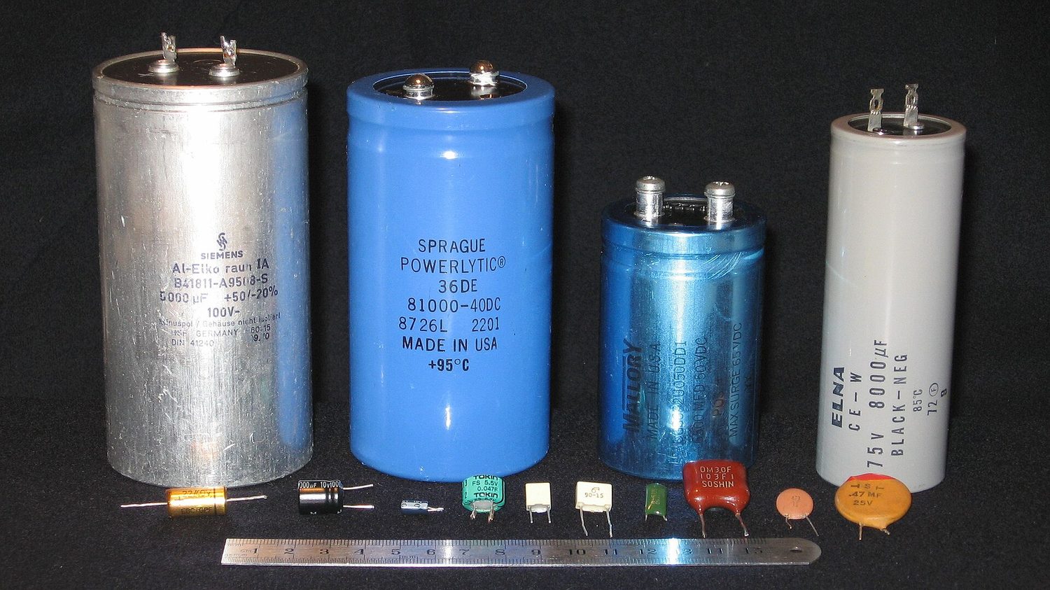
تتراوح المكثفات الفعلية من البراميل الكهربائية الكبيرة (ذات السعة العالية) إلى الأنواع الرقيقة والسيراميكية الصغيرة جداً - من بيكوفاراد حتى مليفاراد
دمج المكثفات
المكثافات المتصلة توازياً تشارك نفس فرق الجهد $V$. الشحنة الكلية هي المجموع:
$$Q_{\text{total}} = C_{1} V + C_{2} V + \ldots, \qquad\text{so}\qquad C_{\text{parallel}} = C_{1} + C_{2} + \ldots$$
التوصيل التوازي يعطي سعة أكبر من أي مكثف على حدة.
المكثفات المتصلة توازلاً تشارك نفس فرق الجهد؛ الشحنات تُجمع
المكثافات المتصلة على التوالي تحمل نفس الشحنة$Q$. فرق الجهد الكلي هو المجموع:
التوصيل على التوالي يعطي سعة أصغر من أي مكثف على حدة.
المكثفات المتصلة على التوالي تحمل نفس الشحنة؛ فروقات الجهد تُجمع
ملحوظة: هذه القواعد هي عكس قواعد المقاومات (المقاومات تُجمع على التوالي؛ المكثفات تُجمع توازلاً)، لأن $C = Q/V$ تحتوي على $V$ في المقام بينما يحتوي $R = V/I$ على $I$ في المقام.
اشتقاق القاعدتين
"اشتق تعبيراً للسعة المركبة" هو سؤال أثبت أن، ومخطط الدرجات يريد عرض الفيزياء وليس مجرد الجبر.
على التوالي. المكثفات تحمل نفس الشحنة$Q$: الصفيحة المتصلة بالقطب الموجب تفقد إلكتروناتها للصفيحة البعيدة للمكثف التالي، لذا كل صفيحة في السلسلة تحمل $\pm Q$. فروقات الجهد تُجمع: $V = V_{1} + V_{2}$. مع $V_{1} = Q/C_{1}$ و$V_{2} = Q/C_{2}$، والتركيبة المعرّفة بواسطة $V = Q/C$، بقسمة الطرفين على $Q$ نحصل على $1/C = 1/C_{1} + 1/C_{2}$.
توازياً. المكثفات لها نفس فرق الجهد$V$، لأن كل منها متصل مباشرة عبر المصدر. الشحنات تُجمع: $Q = Q_{1} + Q_{2} = C_{1}V + C_{2}V$، و$Q = CV$ للتركيب، لذا $C = C_{1} + C_{2}$.
مكثفان متصلان على التوالي يعطيان دائماً أقل من الأصغر منهما؛ مكثفان متساويان $C$ يعطيان $C/2$ على التوالي و$2C$ توازلاً.
تُختزل الشبكة خطوة بخطوة: اجمع الزوج التوازي أولاً، ثم الزوج التوالي
مثال محلول. مكثف قيمته $6.0\ \mu\text{F}$ متصل على التوالي مع زوج توازلي قيمتي $2.0\ \mu\text{F}$ و$4.0\ \mu\text{F}$. أوجد السعة الكلية، والشحنة على كل مكثف عندما يُطبق جهد $12\ \text{V}$ على الشبكة.
الزوج التوازي: $2.0 + 4.0 = 6.0\ \mu\text{F}$. على التوالي مع $6.0\ \mu\text{F}$: $1/C = 1/6.0 + 1/6.0$، لذا $C = 3.0\ \mu\text{F}$. الشحنة الكلية $Q = CV = (3.0 \times 10^{-6})(12) = 3.6 \times 10^{-5}\ \text{C}$: هذه هي الشحنة على المكثف $6.0\ \mu\text{F}$ (توالي، نفس الشحنة)، وهي مقسومة على الزوج التوازي بنسبة سعاته (نفس فرق الجهد، $6.0\ \text{V}$ على كل واحد): المكثف $2.0\ \mu\text{F}$ يحمل $1.2 \times 10^{-5}\ \text{C}$ والمكثف $4.0\ \mu\text{F}$ يحمل $2.4 \times 10^{-5}\ \text{C}$. تحقق: مجموعهما يساوي $3.6 \times 10^{-5}\ \text{C}$.
مثال محلول. مكثفان X و Y، سعة كل منهما $C$، متصلان على التوالي عبر مصدر جهد $V$؛ مكثفان P و Q، سعة كل منهما $C$، متصلان توازلاً عبر نفس المصدر. قارن الشحنة المسحوبة من كل مصدر والطاقة المخزنة في كل ترتيب.
السلسلة: $C_{\text{s}} = C/2$، الشحنة $Q_{\text{s}} = CV/2$، الطاقة $\tfrac{1}{2} C_{\text{s}} V^{2} = CV^{2}/4$. التوازي: $C_{\text{p}} = 2C$، الشحنة $2CV$، الطاقة $CV^{2}$. arrangement التوازي يسحب أربع مرات الشحنة ويخزن أربع مرات الطاقة، لأن عند نفس جهد المصدر تكون الطاقة $\tfrac{1}{2} C V^{2}$ والسعة أكبر بأربعة أضعاف. عند السؤال عن أي arrangement يخزن طاقة أكثر من مصدر معين، الإجابة دائمًا هي التوازي.
Explore · استكشف
Capacitance · السعة
Q = C·V
Charge stored is proportional to voltage — the gradient is the capacitance C. · الشحنة المخزنة تناسب طردياً مع الجهد — الميل يمثل السعة C.
Source: Cambridge International syllabus · المصدر: منهج كامبريدج الدولي
English
Charging a capacitor from $0$ to $Q$ needs work, because each extra bit of charge is pushed against the p.d. already there. When the charge is $q$, the p.d. is $V(q) = q/C$, so adding a small charge $dq$ needs work $V\,dq$. The total work is
Worked example. The graph of charge $Q$ against p.d. $V$ for a capacitor is a straight line through the origin passing through $(10\ \text{V},\ 1.2 \times 10^{-3}\ \text{C})$. Find the capacitance and the energy stored at $10\ \text{V}$, and then the extra energy stored when the p.d. is raised to $12\ \text{V}$.
The gradient of $Q$ against $V$ is $C = 1.2 \times 10^{-3}/10 = 1.2 \times 10^{-4}\ \text{F} = 120\ \mu\text{F}$. Energy is the area under the line: $\tfrac{1}{2}QV = \tfrac{1}{2}(1.2 \times 10^{-3})(10) = 6.0 \times 10^{-3}\ \text{J}$. At $12\ \text{V}$: $\tfrac{1}{2}CV^{2} = \tfrac{1}{2}(1.2 \times 10^{-4})(12)^{2} = 8.6 \times 10^{-3}\ \text{J}$, so the extra energy is $2.6 \times 10^{-3}\ \text{J}$. Do not find the extra energy from the extra charge as $\tfrac{1}{2}(\Delta Q)V$: energy is not proportional to charge, so subtract the two areas.
Reading the $Q$–$V$ graph
A plot of $V$ against $Q$ is a straight line through the origin with gradient $1/C$. The energy stored is the area under the line up to a given charge $Q$, which is the triangle $\tfrac{1}{2} Q V$. The factor $\tfrac{1}{2}$ is there because the average p.d. during charging is $V/2$ (it grows from zero to $V$), not $V$.
Why charging is "half efficient"
Connect a capacitor $C$ to an ideal battery of e.m.f. $V$ through a wire. The capacitor stores $\tfrac{1}{2} C V^{2}$, but the battery supplies charge $Q = CV$ at e.m.f. $V$, giving out $QV = CV^{2}$. The other half is lost as heat in the wire — whatever the wire's resistance.
Sharing charge between capacitors
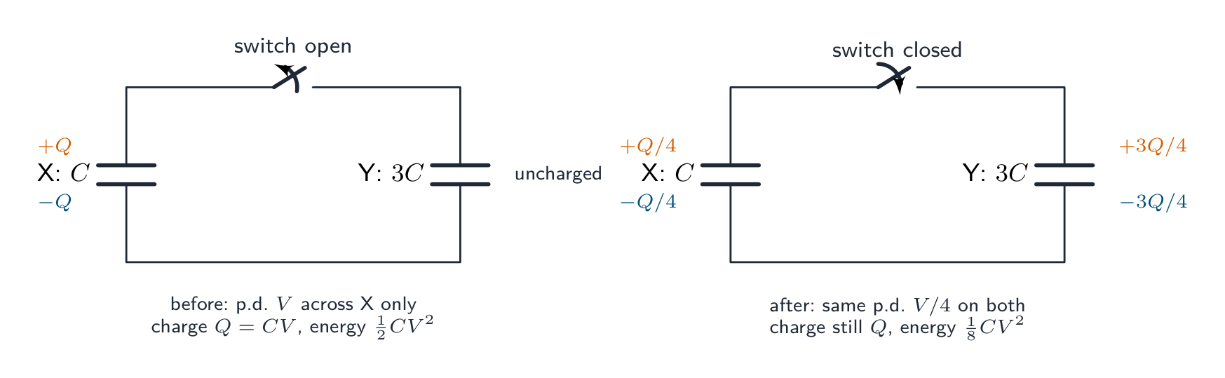
A fully charged capacitor X (capacitance $C$, p.d. $V$, charge $Q = CV$) is disconnected from its supply and connected across an uncharged capacitor Y of capacitance $3C$. Charge flows until the two p.d.s are equal. Two principles settle everything:
Charge is conserved. The total charge is still $Q$, now spread over a parallel pair of total capacitance $4C$, so the common p.d. is $V' = Q/(4C) = V/4$. X keeps $Q/4$ and Y takes $3Q/4$ (charge in the ratio of the capacitances, since the p.d. is the same).
Energy is not conserved. Before: $\tfrac{1}{2} C V^{2}$. After: $\tfrac{1}{2}(4C)(V/4)^{2} = \tfrac{1}{8} C V^{2}$. Three-quarters of the energy has gone: it is dissipated 耗散 as heat in the connecting wires (and as a spark or electromagnetic radiation) while the charge moves, however small the resistance.
Worked example. A $220\ \mu\text{F}$ capacitor charged to $9.0\ \text{V}$ is connected across an uncharged $440\ \mu\text{F}$ capacitor. Find the final p.d. and the energy lost.
$Q = CV = (220 \times 10^{-6})(9.0) = 1.98 \times 10^{-3}\ \text{C}$; total capacitance $660\ \mu\text{F}$, so $V' = 1.98 \times 10^{-3}/(660 \times 10^{-6}) = 3.0\ \text{V}$. Energy before: $\tfrac{1}{2}(220 \times 10^{-6})(9.0)^{2} = 8.9 \times 10^{-3}\ \text{J}$; after: $\tfrac{1}{2}(660 \times 10^{-6})(3.0)^{2} = 3.0 \times 10^{-3}\ \text{J}$; lost: $5.9 \times 10^{-3}\ \text{J}$, two-thirds of the original. A capacitor connected to another of capacitance $kC$ always loses the fraction $k/(k+1)$.
العربية
شحن مكثف من $0$ إلى $Q$ يتطلب شغلًا، لأن كل قطعة إضافية من الشحنة تُدفع ضد فرق الجهد (p.d.) الموجود بالفعل. عندما تكون الشحنة $q$، يكون فرق الجهد $V(q) = q/C$، لذا فإن إضافة شحنة صغيرة $dq$ تتطلب شغلًا $V\,dq$. الشغل الكلي هو
مثال محلول. الرسم البياني للشحنة $Q$ مقابل فرق الجهد $V$ لمكثف هو خط مستقيم يمر بنقطة الأصل ويمر عبر $(10\ \text{V},\ 1.2 \times 10^{-3}\ \text{C})$. أوجد السعة والطاقة المخزنة عند $10\ \text{V}$، ثم الطاقة الإضافية المخزنة عندما يُرفع فرق الجهد إلى $12\ \text{V}$.
الميل لـ $Q$ مقابل $V$ هو $C = 1.2 \times 10^{-3}/10 = 1.2 \times 10^{-4}\ \text{F} = 120\ \mu\text{F}$. الطاقة هي المساحة تحت الخط: $\tfrac{1}{2}QV = \tfrac{1}{2}(1.2 \times 10^{-3})(10) = 6.0 \times 10^{-3}\ \text{J}$. عند $12\ \text{V}$: $\tfrac{1}{2}CV^{2} = \tfrac{1}{2}(1.2 \times 10^{-4})(12)^{2} = 8.6 \times 10^{-3}\ \text{J}$، لذا فإن الطاقة الإضافية هي $2.6 \times 10^{-3}\ \text{J}$. لا تجد الطاقة الإضافية من الشحنة الإضافية كـ $\tfrac{1}{2}(\Delta Q)V$: الطاقة ليست متناسبة مع الشحنة، لذا اطرح المساحتين.
قراءة الرسم البياني $Q$–$V$
رسم بياني لـ $V$ مقابل $Q$ هو خط مستقيم يمر بنقطة الأصل بميل $1/C$. الطاقة المخزنة هي المساحة تحت الخط حتى شحنة معينة $Q$، وهي المثلث $\tfrac{1}{2} Q V$. العامل $\tfrac{1}{2}$ موجود لأن متوسط فرق الجهد أثناء الشحن هو $V/2$ (يتزايد من الصفر إلى $V$)، وليس $V$.
الطاقة المخزنة هي المساحة تحت خط الجهد-الشحنة (المثلث $\tfrac{1}{2}QV$)
لماذا الشحن "نصف فعال"
قم بتوصيل مكثف $C$ ببطارية مثالية ذات قوة دافعة كهربائية e.m.f. $V$ عبر سلك. يخزن المكثف $\tfrac{1}{2} C V^{2}$، لكن البطارية تزود شحنة $Q = CV$ بقوة دافعة كهربائية e.m.f. $V$، مما يعطي ⟨⟩$QV = CV^{2}$. النصف الآخر يتحول إلى حرارة في السلك — بغض النظر عن مقاومة السلك.
مشاركة الشحنة بين المكثفات
توصيل مكثف مشحون بآخر غير مشحون: الشحنة محفوظة، يتساوى فرق الجهد، وتضيع الطاقة
مكثف X مشحون بالكامل (سعة $C$، فرق جهد $V$، شحنة $Q = CV$) مفصول عن مصدره ومتصل عبر مكثف Y غير مشحون بسعة $3C$. تتدفق الشحنة حتى يتساوى كلا فرقَي الجهد. مبدأان يحددان كل شيء:
الشحنة محفوظة. إجمالي الشحنة لا يزال $Q$، موزع الآن على زوج توازي بسعة كلية $4C$، لذا فإن فرق الجهد المشترك هو $V' = Q/(4C) = V/4$. يحتفظ X بـ $Q/4$ ويأخذ Y $3Q/4$ (الشحنة في نسبة السعات، بما أن فرق الجهد متساوٍ).
الطاقة غير محفوظة. قبل: $\tfrac{1}{2} C V^{2}$. بعد: $\tfrac{1}{2}(4C)(V/4)^{2} = \tfrac{1}{8} C V^{2}$. ذهب ثلاثة أرباع الطاقة: وهي متبددة كحرارة في الأسلاك المتصلة (وكبرق أو إشعاع كهرومغناطيسي) أثناء حركة الشحنة، مهما كانت المقاومة صغيرة.
مثال محلول. مكثف سعة $220\ \mu\text{F}$ مشحون بجهد $9.0\ \text{V}$ مُوصل عبر مكثف آخر غير مشحون بسعة $440\ \mu\text{F}$. أوجد فرق الجهد النهائي والطاقة المفقودة.
Capacitor discharging through a resistor · تفريغ المكثف عبر مقاومة
Syllabus · المنهج
English
analyse graphs of the variation with time of potential difference, charge and current for a capacitor discharging through a resistor
recall and use $\tau = RC$ for the time constant for a capacitor discharging through a resistor
use equations of the form $x = x_0 e^{-(t/RC)}$ where $x$ could represent current, charge or potential difference for a capacitor discharging through a resistor
العربية
حلل الرسوم البيانية التي توضح تغير فرق الجهد والشحنة والتيار مع الزمن لمكثف يتم تفريغه عبر مقاومة
استذكر واستخدم $\tau = RC$ لحساب ثابت الزمن لمكثف يتم تفريغه عبر مقاومة
استخدم معادلات من الشكل $x = x_0 e^{-(t/RC)}$ حيث يمكن أن يمثل $x$ التيار أو الشحنة أو فرق الجهد لمكثف يتم تفريغه عبر مقاومة
Source: Cambridge International syllabus · المصدر: منهج كامبريدج الدولي
English
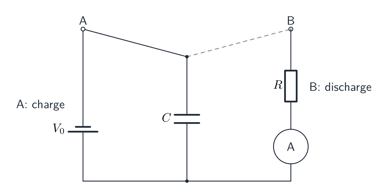
A capacitor $C$ charged to $V_{0}$ is connected through a switch to a resistor 电阻器 of resistance 电阻$R$. When the switch closes at $t = 0$, the capacitor discharges.
Setting up the equation
By Kirchhoff's second law 基尔霍夫第二定律 around the loop, $V_{C} = V_{R}$. Using $V_{C} = Q/C$, $V_{R} = IR$ and $I = -dQ/dt$:
$$\frac{Q}{C} = -R \frac{dQ}{dt}.$$
This is solved by an exponential decay 指数衰减 with time constant $RC$.
Discharge equations
Charge $Q$, p.d. $V$ and current $I$ all decay exponentially with the same time constant:
$$Q = Q_{0} e^{-t / (RC)}, \qquad V = V_{0} e^{-t / (RC)}, \qquad I = I_{0} e^{-t / (RC)},$$
with $I_{0} = V_{0}/R$.
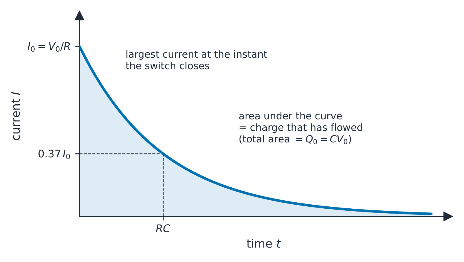
Reading the three graphs. All three curves have the same shape and the same time constant, so one measurement of $\tau$ from any of them gives $RC$. The current is largest the instant the switch closes, $I_{0} = V_{0}/R$, because the full p.d. $V_{0}$ is then across the resistor; it falls as the p.d. falls. The area under the $I$–$t$ graph is the charge that has flowed, so the total area is $Q_{0} = CV_{0}$, and the charge that flows in the first time constant is $Q_{0}(1 - e^{-1}) = 0.63\,Q_{0}$. The gradient of the $Q$–$t$ graph is $-I$: steepest at the start, flattening as the current dies away. (During charging through a resistor the current has the same decaying shape, while $V$ and $Q$ rise as $V_{0}(1 - e^{-t/RC})$, the mirror image of the discharge curve.)
Time constant
$$\tau = RC$$
is the time constant 时间常数 (in seconds: $\Omega \cdot \text{F} = \text{s}$). It is the time for a decaying quantity to fall to $1/e \approx 0.37$ (about 37%) of its starting value. After $2\tau$ it is at about 13.5%; after $5\tau$, below 1%.
Worked example. A $100\ \mu\text{F}$ capacitor charged to $12\ \text{V}$ is discharged through a $47\ \text{k}\Omega$ resistor. Find the time constant and the voltage after one time constant.
After one time constant the voltage falls to $1/e$ of its start: $V = 12 \times 0.37 \approx 4.4\ \text{V}$.
Worked example. A $470\ \mu\text{F}$ capacitor is charged to $24\ \text{V}$ and then discharged through a $5.6\ \text{k}\Omega$ resistor. Find (a) the initial charge and energy, (b) the time constant and the initial current, (c) the p.d. after $4.0\ \text{s}$, (d) the time for the p.d. to fall to $6.0\ \text{V}$.
Keep the time constant unrounded ($2.632\ \text{s}$) inside the calculation and round only the answers. The rearrangement in (d) is the one most often asked and most often botched: $\ln(V/V_{0})$ is negative, so $t$ comes out positive.
Worked example. From a discharge graph, the p.d. across a $2200\ \mu\text{F}$ capacitor falls from $6.0\ \text{V}$ to $2.2\ \text{V}$ in $4.5\ \text{s}$. Find the resistance of the resistor.
$2.2/6.0 = 0.367 \approx 1/e$, so $4.5\ \text{s}$ is one time constant: $R = \tau/C = 4.5/(2200 \times 10^{-6}) = 2.0 \times 10^{3}\ \Omega$. If the fall is not to $1/e$, use $RC = -t/\ln(V/V_{0})$; the answer is the same either way.
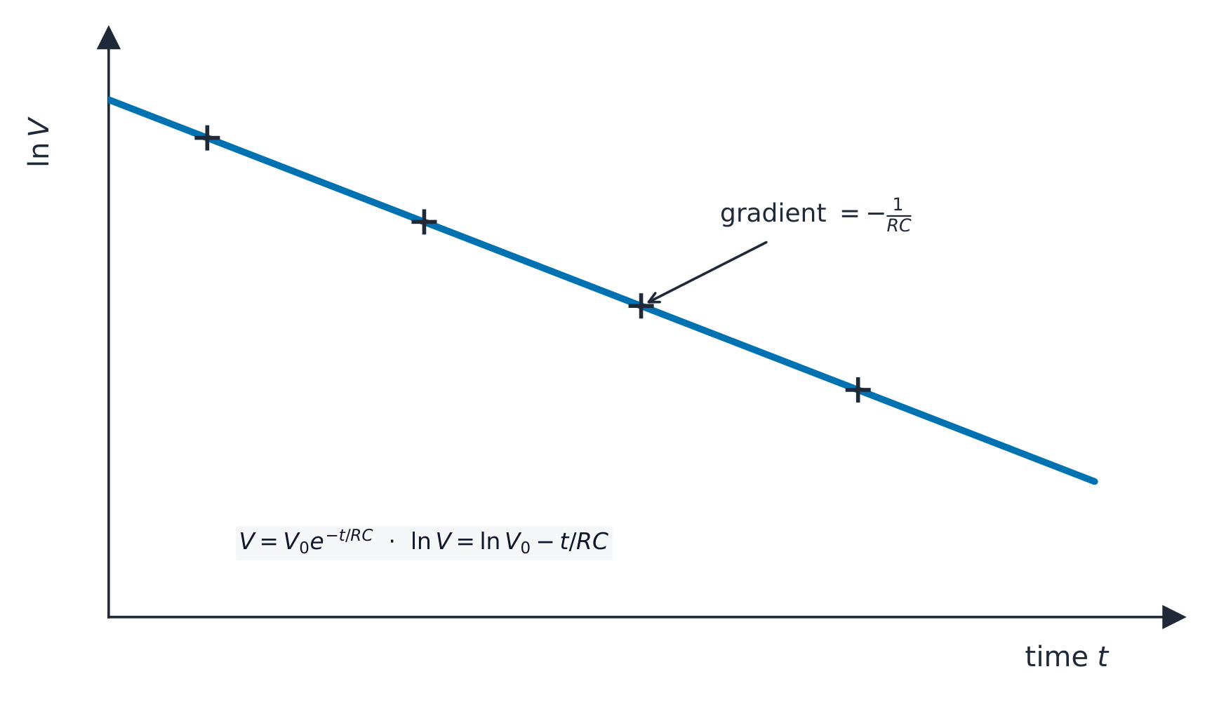
To find $\tau$ from a curve: read the time to fall to $1/e$ of the start. Or take logs: $\ln(V/V_{0}) = -t/(RC)$, so a plot of $\ln V$ against $t$ is a straight line with gradient $-1/(RC)$.
Using the logarithmic graph. In an experiment, plot $\ln V$ (or $\ln I$) on the $y$-axis against $t$. The points should lie on a straight line: its gradient is $-1/(RC)$, so $RC = -1/\text{gradient}$, and its intercept 截距 on the $\ln V$ axis is $\ln V_{0}$. A straight line is the test that the decay really is exponential; a curve means it is not. Take the gradient from two points far apart on the best-fit line, not from two data points, and quote $RC$ in seconds.
Reading graphs during discharge
$Q$ against $V_{C}$: since $Q = C V$ always, this is a straight line through the origin with gradient $C$. Discharge moves the point from $(V_{0}, Q_{0})$ down to $(0,0)$.
$I$ against $V_{C}$: since $I = V_{C}/R$, this is a straight line through the origin with gradient $1/R$, so you can find $R$.
Common exam questions
Given a discharge curve $V(t)$ or $Q(t)$:
read the start value $V_{0}$ or $Q_{0}$ at $t = 0$.
read the time to fall to $V_{0}/e$ → time constant $\tau = RC$.
given $R$, find $C = \tau / R$ (or the other way round).
predict a later value with the exponential formula.
A capacitor as a smoothing component
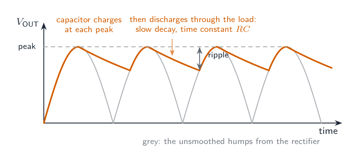
A rectifier 整流器 (Topic 21) turns an alternating voltage into a series of positive humps. A capacitor connected across the load smooths them. Near each peak 峰值 the diodes conduct and the capacitor charges to the peak voltage; as the supply voltage falls away the diodes stop conducting and the capacitor discharges through the load resistor, holding the output up until the next hump rises above it and recharges the capacitor. The output therefore falls only a little between peaks; the rise and fall that remains is the ripple 纹波.
How much it falls depends on the time constant of the discharge, $RC$, compared with the time between peaks. A larger capacitance, or a larger load resistance (a smaller load current), gives a larger $RC$, a slower decay and a smaller ripple; a heavily loaded supply (small $R$) has a larger ripple. Asked to sketch the smoothed output, draw it touching each peak, decaying slightly between them, and never falling to zero.
العربية
مكثف $C$ مشحون بجهد $V_{0}$ مُوصل عبر مفتاح إلى مقاومةمقاومتها$R$. عند إغلاق المفتاح في $t = 0$، يتم تفريغ المكثف.
يشحن المكثف عبر المفتاح A، ثم يفرغ عبر المقاومة عبر المفتاح B
إعداد المعادلة
بواسطة قانون كيرشوف الثاني حول الحلقة، $V_{C} = V_{R}$. باستخدام $V_{C} = Q/C$، $V_{R} = IR$ و$I = -dQ/dt$:
$$Q = Q_{0} e^{-t / (RC)}, \qquad V = V_{0} e^{-t / (RC)}, \qquad I = I_{0} e^{-t / (RC)},$$
مع $I_{0} = V_{0}/R$.
يبدأ تيار التفريغ عند $V_0/R$ وينهار بنفس الثابت الزمني؛ المساحة تحت المنحنى هي الشحنة التي مرّت
قراءة الرسوم البيانية الثلاثة. جميع المنحنيات الثلاث لها نفس الشكل ونفس الثابت الزمني، لذا فإن قياس واحد لـ $\tau$ من أي منها يعطي $RC$. التيار يكون أكبر لحظة إغلاق المفتاح، $I_{0} = V_{0}/R$، لأن فرق الجهد الكامل $V_{0}$ يكون آنذاك عبر المقاومة؛ وينخفض مع انخفاض فرق الجهد. المساحة تحت المنحنى $I$–$t$ هي الشحنة التي مرت، لذا المساحة الكلية هي $Q_{0} = CV_{0}$، والشحنة التي تمر في أول ثابت زمني هي $Q_{0}(1 - e^{-1}) = 0.63\,Q_{0}$. الميل للمنحنى $Q$–$t$ هو $-I$: حاد في البداية ويستوي كلما خفت شدة التيار. (أثناء الشحن عبر مقاومة يكون للتيار نفس الشكل المتناقص، بينما $V$ و$Q$ ترتفع كما $V_{0}(1 - e^{-t/RC})$، وهو انعكاس المرآة لمنحنى التفريغ).
تتناقص الشحنة أسيًا أثناء التفريغ، لتصل إلى $Q_0/e$ بعد ثابت زمني واحد $RC$
الثابت الزمني
$$\tau = RC$$
هو الثابت الزمني (بالثواني: $\Omega \cdot \text{F} = \text{s}$). هو الوقت الذي يستغرقه الكمية المتناقصة لتصل إلى $1/e \approx 0.37$ (حوالي 37%) من قيمتها الأولية. بعد $2\tau$ تكون حوالي 13.5%؛ وبعد $5\tau$، أقل من 1%.
مثال محلول. مكثف سعته $100\ \mu\text{F}$ مشحون بجهد $12\ \text{V}$ يتم تفريغه عبر مقاومة $47\ \text{k}\Omega$. أوجد الثابت الزمني والجهد بعد ثابت زمني واحد.
بعد ثابت زمني واحد، ينخفض الجهد إلى $1/e$ من بدايته: $V = 12 \times 0.37 \approx 4.4\ \text{V}$.
مثال محلول. مكثف سعته $470\ \mu\text{F}$ مشحون بجهد $24\ \text{V}$ ثم يتم تفريغه عبر مقاومة $5.6\ \text{k}\Omega$. أوجد (أ) الشحنة الأولية والطاقة، (ب) الثابت الزمني والتيار الأولي، (ج) فرق الجهد بعد $4.0\ \text{s}$، (د) الوقت اللازم لفرق الجهد ليصل إلى $6.0\ \text{V}$.
احتفظ بالثابت الزمني غير مقرب ($2.632\ \text{s}$) داخل الحساب وقم بالتقريب فقط للإجابات. إعادة الترتيب في (د) هي الأكثر طلبًا والأكثر شيوعًا في الخطأ: $\ln(V/V_{0})$ سالب، لذا فإن $t$ يصبح موجبًا.
مثال محلول. من رسم بياني للتفريغ، انخفض فرق الجهد عبر مكثف سعته $2200\ \mu\text{F}$ من $6.0\ \text{V}$ إلى $2.2\ \text{V}$ في $4.5\ \text{s}$. أوجد مقاومة المقاومة.
$2.2/6.0 = 0.367 \approx 1/e$، لذا $4.5\ \text{s}$ هو ثابت زمني واحد: $R = \tau/C = 4.5/(2200 \times 10^{-6}) = 2.0 \times 10^{3}\ \Omega$. إذا لم يكن الانخفاض إلى $1/e$، استخدم $RC = -t/\ln(V/V_{0})$؛ الإجابة ستكون متساوية في الحالتين.
لإيجاد $\tau$ من منحنى: اقرأ الزمن اللازم للوصول إلى $1/e$ من البداية. أو خذ اللوغاريتمات: $\ln(V/V_{0}) = -t/(RC)$، لذا فإن رسم بياني لـ $\ln V$ مقابل $t$ هو خط مستقيم بميل $-1/(RC)$.
رسم بياني لـ $\ln V$ مقابل الزمن هو خط مستقيم بميل $-1/(RC)$
استخدام الرسم البياني اللوغاريتمي. في تجربة، ارسم $\ln V$ (أو $\ln I$) على المحور $y$ مقابل $t$. يجب أن تقع النقاط على خط مستقيم: ميله هو $-1/(RC)$، لذا $RC = -1/\text{gradient}$، وقاطعه على المحور $\ln V$ هو $\ln V_{0}$. الخط المستقيم هو الاختبار الذي يؤكد أن التناقص فعلاً أسي؛ والمنحنى يعني أنه ليس كذلك. احسب الميل من نقطتين بعيدتين على خط أفضل ملاءمة، وليس من نقطتي بيانات، وأدرج $RC$ بالثواني.
قراءة الرسوم البيانية أثناء التفريغ
$Q$ مقابل $V_{C}$: بما أن $Q = C V$ دائماً، فهذا خط مستقيم يمر بنقطة الأصل بميل $C$. عملية التفريغ تحرك النقطة من $(V_{0}, Q_{0})$ إلى الأسفل نحو $(0,0)$.
$I$ مقابل $V_{C}$: بما أن $I = V_{C}/R$، فهذا خط مستقيم يمر بنقطة الأصل بميل $1/R$، لذا يمكنك إيجاد $R$.
أسئلة الامتحانات الشائعة
بموجب منحنى التفريغ $V(t)$ أو $Q(t)$:
اقرأ القيمة الابتدائية $V_{0}$ أو $Q_{0}$ عند $t = 0$.
اقرأ الزمن اللازم للنزول إلى $V_{0}/e$ → الثابت الزمني $\tau = RC$.
بمعلومية $R$، أوجد $C = \tau / R$ (أو العكس).
تنبأ بقيمة لاحقة باستخدام الصيغة الأسية.
المكثف كعنصر تنعيم
يتشحن المكثف عبر الحمل عند كل قمة ويتفريغ عبر الحمل فيما بينها، مما يحول القمم إلى مخرج شبه ثابت مع تموج صغير
المصحح (الموضوع 21) يحول الجوتر المتردد إلى سلسلة من القمم الموجبة. المكثف المتصل عبر الحمل ينعمها. بالقرب من كل قمة، تتدفق الديودات وتتشحن السعة إلى جهد القمة؛ عندما ينخفض جهد المصدر، تتوقف الديودات عن التدفق ويتم تفريغ المكثف عبر مقاومة الحمل، مما يحافظ على المخرج مرتفعًا حتى ترتفع القمة التالية فوقه وتشحن المكثف مرة أخرى. لذلك ينخفض المخرج قليلاً فقط بين القمم؛ الارتفاع والانخفاض المتبقي هو التموج.
يعتمد مقدار الانخفاض على الثابت الزمني للتفريغ، $RC$، مقارنة بالزمن بين القمم. السعة الأكبر، أو مقاومة الحمل الأكبر (تيار حمل أصغر)، تعطي ثابتًا زمنيًا $RC$ أكبر، وتناقصًا أبطأ وتموجًا أصغر؛ المصدر المحمل بشدة (ثابت زمني $R$ صغير) له تموج أكبر. عند الطلب لرسم المخرج المُنعم، ارسمه يلمس كل قمة، ويتناقص قليلاً بينها، ولا ينخفض أبدًا إلى الصفر.
Explore · استكشف
Charge / discharge curve · منحنى الشحن/التفريغ
The voltage rises (or decays) exponentially with time constant τ = RC. · يرتفع الجهد (أو يتناقص) أسياً مع ثابت زمني τ = RC.
Explore · استكشف
Discharging a capacitor · تفريغ مكثف
Q = Q₀·bᵗ
Charge decays exponentially through the resistor. · الشحنة تنخفض أسياً عبر المقاومة.
Definitions the examiner accepts · التعريفات التي يقبلها المصحح
English
A definition question is marked against fixed wording. Learn these exactly, and give one answer only.
Term
Definition
capacitance (parallel-plate capacitor)
the charge on one plate per unit potential difference between the plates
capacitance (isolated conductor)
the charge on the conductor per unit potential
farad
one coulomb per volt
capacitors in series
the same charge on each; the p.d.s add; $1/C = 1/C_{1} + 1/C_{2}$
capacitors in parallel
the same p.d. across each; the charges add; $C = C_{1} + C_{2}$
energy stored
the work done in charging the capacitor, equal to the area under the potential–charge graph; $W = \tfrac{1}{2}QV = \tfrac{1}{2}CV^{2}$
time constant
the product $RC$; the time for the charge (or p.d., or current) to fall to $1/e$ of its initial value
العربية
تُصنّف أسئلة التعريف بناءً على صياغة ثابتة. احفظ هذه التعريفات بدقة، وقدم إجابة واحدة فقط.
مصطلح
تعريف
السعة (المكثف صفيحي)
الشحنة على لوح واحد لكل وحدة فرق جهد بين اللوحين
السعة (الموصل المعزول)
الشحنة على الموصل لكل وحدة جهد
الفاراد
كولوم واحد لكل فولت
المكثفات على التوالي
نفس الشحنة على كل واحد؛ مجموع فروق الجهد؛ $1/C = 1/C_{1} + 1/C_{2}$
مكثفات على التوازي
نفس فرق الجهد عبر كل منها؛ تتجمع الشحنات؛ $C = C_{1} + C_{2}$
الطاقة المخزنة
الشغل المبذول في شحن المكثف، يساوي المساحة تحت منحنى الجهد–الشحنة؛ $W = \tfrac{1}{2}QV = \tfrac{1}{2}CV^{2}$
الثابت الزمني
حاصل ضرب $RC$؛ الوقت اللازم لتناقص الشحنة (أو فرق الجهد، أو التيار) إلى $1/e$ قيمتها الابتدائية
19.3
Exam tips · نصائح للامتحان
English
$C = Q/V$ defines capacitance; for an isolated sphere $C = 4\pi\varepsilon_{0} r$. Energy stored $W = \tfrac{1}{2}QV = \tfrac{1}{2}CV^{2} = Q^{2}/2C$: pick the form that uses what you know, and remember that energy is not proportional to charge.
Combine capacitors the opposite way to resistors (parallel add, series reciprocal), and reduce a network one step at a time.
Charge sharing: charge is conserved, energy is not. Find the common p.d. from the total charge and the total capacitance first, then the energies.
Discharge: $x = x_{0} e^{-t/RC}$ for $Q$, $V$ and $I$ alike; $t = -RC \ln(x/x_{0})$; $\tau = RC$ is in seconds ($\Omega \cdot \text{F} = \text{s}$) and is the time to fall to $37\%$, not to zero.
Graphs: the initial current is $V_{0}/R$; the area under $I$–$t$ is charge; the gradient of $Q$–$t$ is $-I$; $\ln V$ against $t$ is a straight line of gradient $-1/(RC)$ and intercept $\ln V_{0}$.
Convert $\mu\text{F}$ and $\text{k}\Omega$ before multiplying: $\text{k}\Omega \times \mu\text{F}$ gives milliseconds, not seconds.
Common mistakes
Defining capacitance as "the charge stored" or "the charge on both plates". It is the charge on one plate per unit p.d. between the plates.
Adding capacitors in series as if they were resistors, or forgetting to invert the reciprocal sum at the end.
After charge sharing, using the supply voltage in $\tfrac{1}{2}CV^{2}$ instead of the new common p.d., or claiming the energy is conserved.
Drawing the discharge current starting from zero. It starts at its largest value, $V_{0}/R$.
Treating $\tau$ as the time to discharge completely; after $5\tau$ about $1\%$ remains.
Dropping the minus sign in $t = -RC \ln(V/V_{0})$ and reporting a negative time.
Finding the extra energy on raising the p.d. from the extra charge alone: subtract two areas (or two $\tfrac{1}{2}CV^{2}$ values).
Sketching a smoothed output that falls to zero between peaks, or saying a larger load resistance gives a larger ripple.
العربية
$C = Q/V$ يُعرّف السعة؛ لكرة معزولة $C = 4\pi\varepsilon_{0} r$. الطاقة المخزنة $W = \tfrac{1}{2}QV = \tfrac{1}{2}CV^{2} = Q^{2}/2C$: اختر الصيغة التي تعتمد على ما تعرفه، وتذكر أن الطاقة لا تتناسب طردياً مع الشحنة.
اجمع المكثفات بطريقة عكس المقاومات تماماً (التوازي يجمع، المتسلسل معكوس المجموع)، وقلل الشبكة خطوة بخطوة.
مشاركة الشحنة: الشحنة محفوظة، الطاقة غير محفوظة. أوجد فرق الجهد المشترك من إجمالي الشحنة وإجمالي السعة أولاً، ثم احسب الطاقات.
التفريغ: $x = x_{0} e^{-t/RC}$ لـ $Q$، $V$ و $I$ متشابهة؛ $t = -RC \ln(x/x_{0})$؛ $\tau = RC$ بالثانية ($\Omega \cdot \text{F} = \text{s}$) وهو الوقت للنزول إلى $37\%$، وليس إلى الصفر.
الرسوم البيانية: التيار الابتدائي هو $V_{0}/R$؛ المساحة تحت $I$–$t$ هي الشحنة؛ ميل $Q$–$t$ هو $-I$؛ $\ln V$ مقابل $t$ خط مستقيم بميل $-1/(RC)$ وقطاع $\ln V_{0}$.
حوّل $\mu\text{F}$ و $\text{k}\Omega$ قبل الضرب: $\text{k}\Omega \times \mu\text{F}$ يعطي مللي ثانية، وليس ثوانٍ.
أخطاء شائعة
تعريف السعة بأنها "الشحنة المخزنة" أو "الشحنة على اللوحين معاً". إنها شحنة لوحة واحدة لكل وحدة فرق جهد بين اللوحين.
جمع المكثفات على التوالي وكأنها مقاومات، أو نسيان قلب مجموع المعكوس في النهاية.
بعد مشاركة الشحنة، استخدام جهد المصدر في $\tfrac{1}{2}CV^{2}$ بدلاً من فرق الجهد المشترك الجديد، أو الادعاء بأن الطاقة محفوظة.
رسم تيار التفريغ بدءاً من الصفر. يبدأ من أكبر قيمة له، $V_{0}/R$.
اعتبار $\tau$ وقت التفريغ الكامل؛ بعد $5\tau$ يبقى حوالي $1\%$.
إسقاط إشارة السالب في $t = -RC \ln(V/V_{0})$ والإبلاغ عن زمن سلبي.
إيجاد الطاقة الإضافية عند رفع فرق الجهد من الزيادة في الشحنة وحدها: اطرح مساحتين (أو قيمتي $\tfrac{1}{2}CV^{2}$).
رسم مخطط للإخراج المُمَوَّج ينخفض إلى الصفر بين الذروات، أو القول إن مقاومة حمل أكبر تعطي تموجاً أكبر.
Interactive lessons on this topic · دروس تفاعلية حول هذا الموضوع
Work through it step by step, with instant-check exercises. · ا-working عليه خطوة بخطوة، مع تمارين تحقق فوري.
Pick one and the site follows you — notes, papers, videos and practice all open on it. · اختر واحدًا وسيتبعك الموقع — الملاحظات، الأوراق، الفيديوهات والتدريب جميعها تفتح عليه.
Type to search notes, lessons, code, vocabulary and past-paper questions across every subject. · اكتب للبحث عن ملاحظات، دروس، أكواد، مفردات وأسئلة امتحانات سابقة عبر جميع المواد.